Lecture 2 Protein secondary structure

prediction

Computational Aspects of Molecular Structure

Teresa Przytycka, PhD

Assumptions in secondary structure prediction

•  Goal: classify each residuum as alpha, beta or coil. •  Assumption: Secondary structure of a residuum is

determined by the amino acid at the given position and amino acids at the neighboring.

•  Chameleon sequence: A sequence that assumes different secondary structure depending on the fold context. The longest known chameleon sequence has 11 res.

Chow-Fasman algorithm Chow, P.Y. and Fasman, G.D. Biochemistry (1974) 13,222.

•  Statistical approach based on calculation of

statistical propensities of each residuum to form an α-helix or β-strand

•  Low accuracy (~50%) (accuracy of current methods >75%).

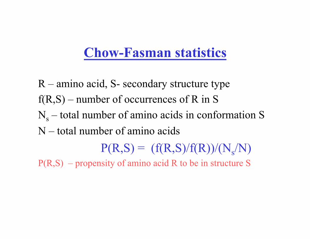
Chow-Fasman statistics

R – amino acid, S- secondary structure type f(R,S) – number of occurrences of R in S Ns – total number of amino acids in conformation S N – total number of amino acids P(R,S) = (f(R,S)/f(R))/(Ns/N) P(R,S) – propensity of amino acid R to be in structure S

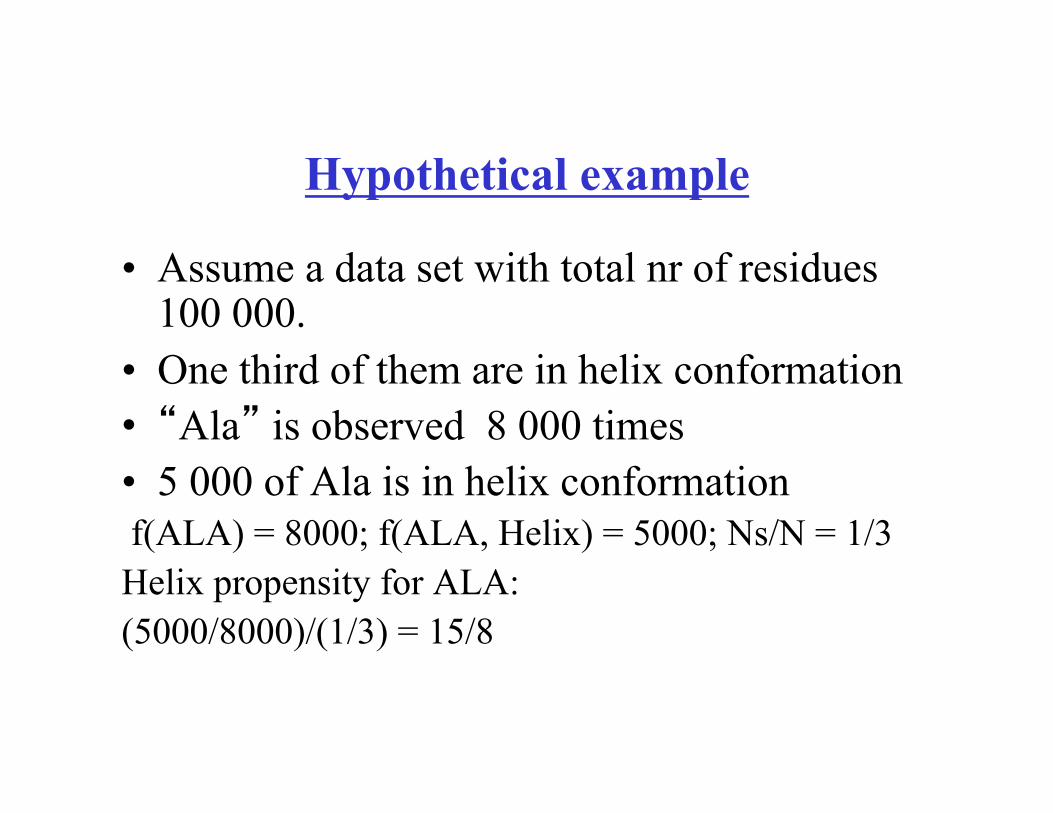
Hypothetical example

•  Assume a data set with total nr of residues 100 000.

•  One third of them are in helix conformation •  “Ala” is observed 8 000 times •  5 000 of Ala is in helix conformation f(ALA) = 8000; f(ALA, Helix) = 5000; Ns/N = 1/3 Helix propensity for ALA: (5000/8000)/(1/3) = 15/8

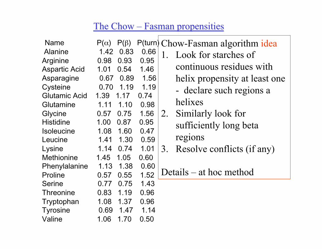
The Chow – Fasman propensities  Name P(α) P(β) P(turn)  Alanine 1.42 0.83 0.66 Arginine 0.98 0.93 0.95 Aspartic Acid 1.01 0.54 1.46 Asparagine 0.67 0.89 1.56 Cysteine 0.70 1.19 1.19 Glutamic Acid 1.39 1.17 0.74 Glutamine 1.11 1.10 0.98 Glycine 0.57 0.75 1.56 Histidine 1.00 0.87 0.95 Isoleucine 1.08 1.60 0.47 Leucine 1.41 1.30 0.59 Lysine 1.14 0.74 1.01 Methionine 1.45 1.05 0.60 Phenylalanine 1.13 1.38 0.60 Proline 0.57 0.55 1.52 Serine 0.77 0.75 1.43 Threonine 0.83 1.19 0.96 Tryptophan 1.08 1.37 0.96 Tyrosine 0.69 1.47 1.14 Valine 1.06 1.70 0.50  

Chow-Fasman algorithm idea 1.  Look for starches of

continuous residues with helix propensity at least one - declare such regions a helixes

2.  Similarly look for sufficiently long beta regions

3.  Resolve conflicts (if any)

Details – at hoc method

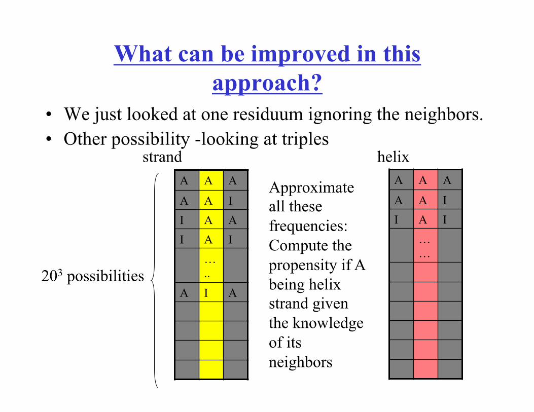
What can be improved in this approach?

•  We just looked at one residuum ignoring the neighbors. •  Other possibility -looking at triples

A A A

A A I I A A I A I

…..

A I A

A A A

A A I I A I

……

Approximate all these frequencies: Compute the propensity if A being helix strand given the knowledge of its neighbors

strand helix

203 possibilities

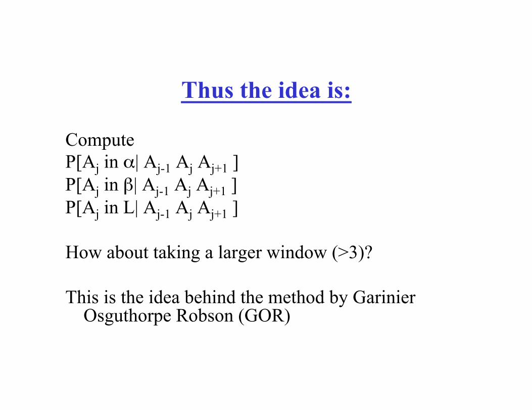
Thus the idea is: Compute P[Aj in α| Aj-1 Aj Aj+1 ] P[Aj in β| Aj-1 Aj Aj+1 ] P[Aj in L| Aj-1 Aj Aj+1 ] How about taking a larger window (>3)? This is the idea behind the method by Garinier

Osguthorpe Robson (GOR)

GOR

Consider window of 17 positions and see how the conformation of the central residuum depends on this residuum and its 18 neighbors (8 in each direction).

Ideally one would consider all possible combinations of these neighbors. This is impossible: would require collecting statistics for 20^17 sequences.

Instead assume the central residuum depends on its neighbors but the neighbors are independent on each other

Implementation :Statistical information derived from proteins of known structure is stored in three (17X20) matrices, one each for α, β, coil

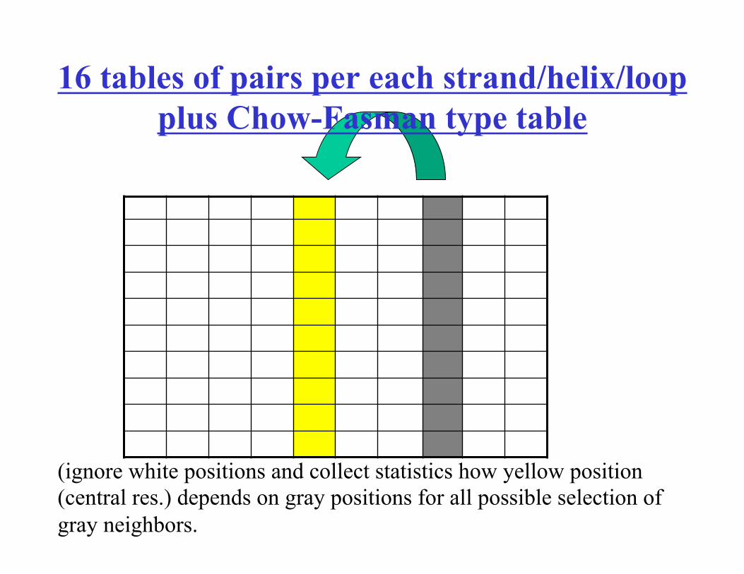
16 tables of pairs per each strand/helix/loop plus Chow-Fasman type table

(ignore white positions and collect statistics how yellow position (central res.) depends on gray positions for all possible selection of gray neighbors.

The final prediction

For every neighbor x of distance 8 or less compute the propensity of a given residuum to be in a secondary structure of a given type (helix, strand, loop) under assumption that x is a particular amino acid.

Sum contribution from all neighbors.

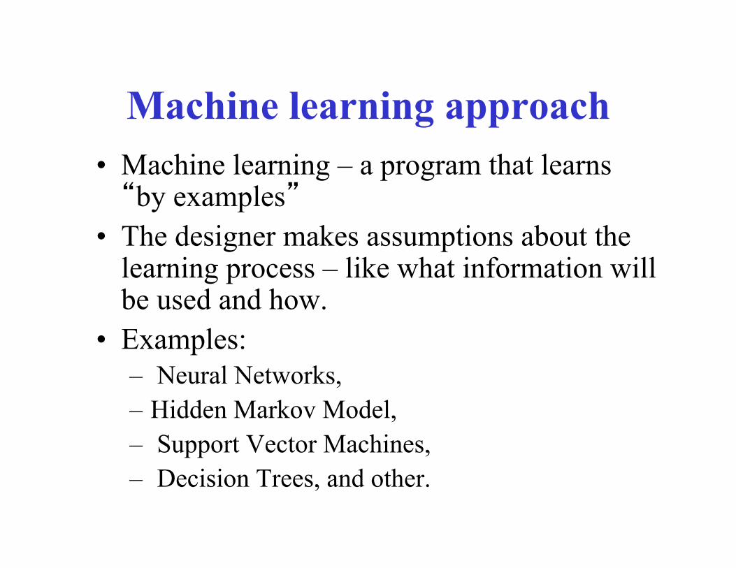
Machine learning approach •  Machine learning – a program that learns “by examples”

•  The designer makes assumptions about the learning process – like what information will be used and how.

•  Examples: –  Neural Networks, – Hidden Markov Model, –  Support Vector Machines, –  Decision Trees, and other.

X

X

X

X

1

2

3

k

..

.

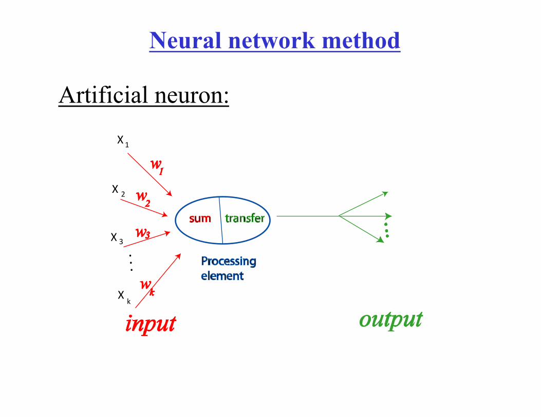
Neural network method

Artificial neuron:

Components of an artificial neuron

•  Weighting factor – A neuron receives many simultaneous inputs. Each input has it’s own relative weight (w)

•  Summation function – Processing in the usually artificial neuron consists of computing weighted sum.

•  Transfer function – the result of the summing function is transferred via transfer function. Transfer function usually compares the weighted sum against some threshold value and may transfer no signal is the value is below the threshold.

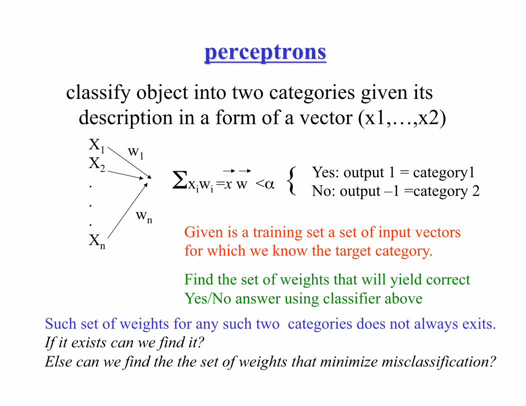
perceptrons

classify object into two categories given its description in a form of a vector (x1,…,x2)

X1 X2 . . . Xn

w1

wn

Σxiwi =x w <α { Yes: output 1 = category1 No: output –1 =category 2

Such set of weights for any such two categories does not always exits. If it exists can we find it? Else can we find the the set of weights that minimize misclassification?

Given is a training set a set of input vectors for which we know the target category.

Find the set of weights that will yield correct Yes/No answer using classifier above

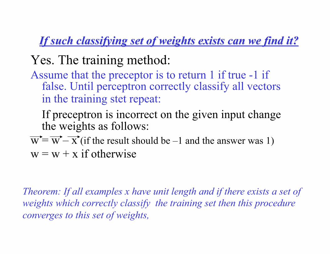
If such classifying set of weights exists can we find it?

Yes. The training method: Assume that the preceptor is to return 1 if true -1 if

false. Until perceptron correctly classify all vectors in the training stet repeat: If preceptron is incorrect on the given input change the weights as follows:

w = w – x (if the result should be –1 and the answer was 1) w = w + x if otherwise

Theorem: If all examples x have unit length and if there exists a set of weights which correctly classify the training set then this procedure converges to this set of weights,

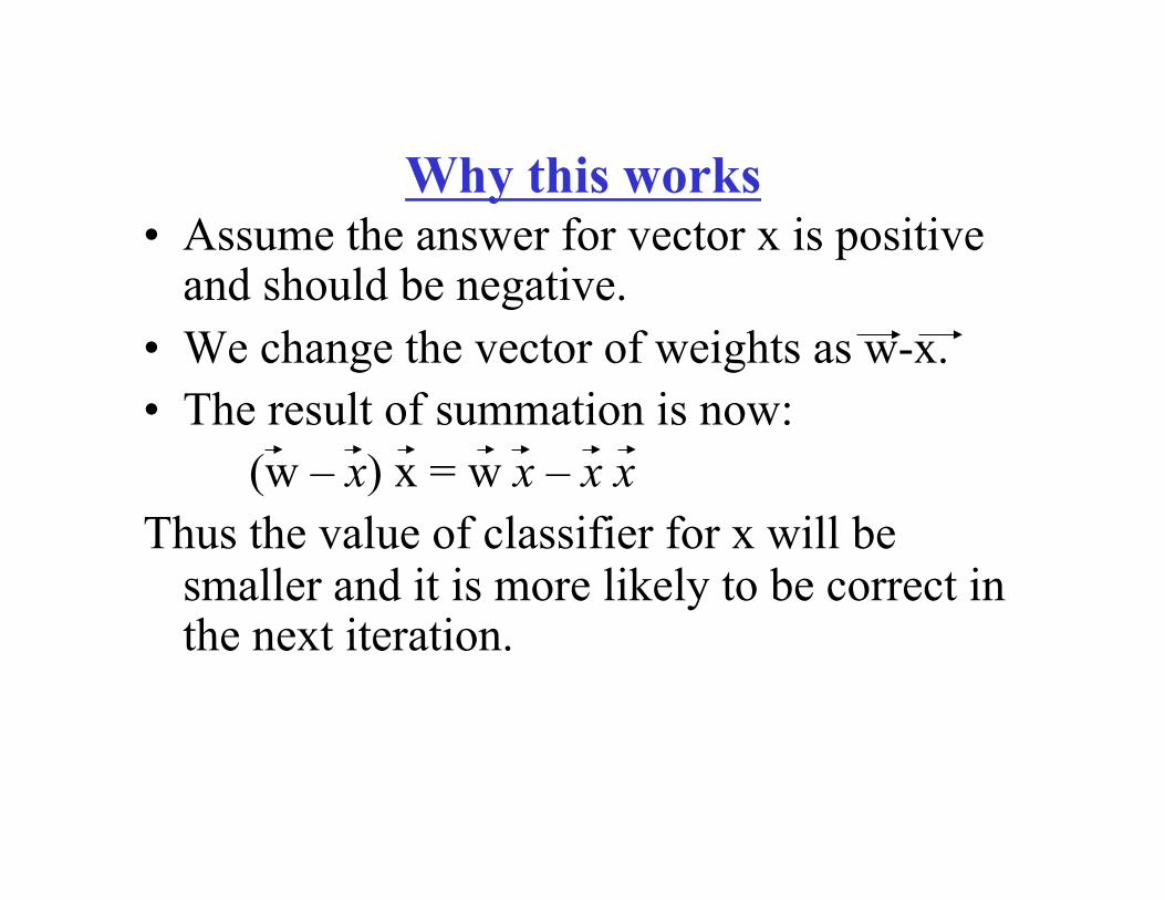
Why this works •  Assume the answer for vector x is positive

and should be negative. •  We change the vector of weights as w-x. •  The result of summation is now: (w – x) x = w x – x x Thus the value of classifier for x will be

smaller and it is more likely to be correct in the next iteration.

If such classifying set of weights does not exists can we find a set of weight that minimize error?

Idea: (We will not discuss details. Recommended reading: Mona Singh’s lecture notes:)

•  Define a function that describes error – a multivariable function with weights as variables

•  Use a method (like gradient descend) that finds a local minimum of the error function (unfortunately this is not a global minimum)

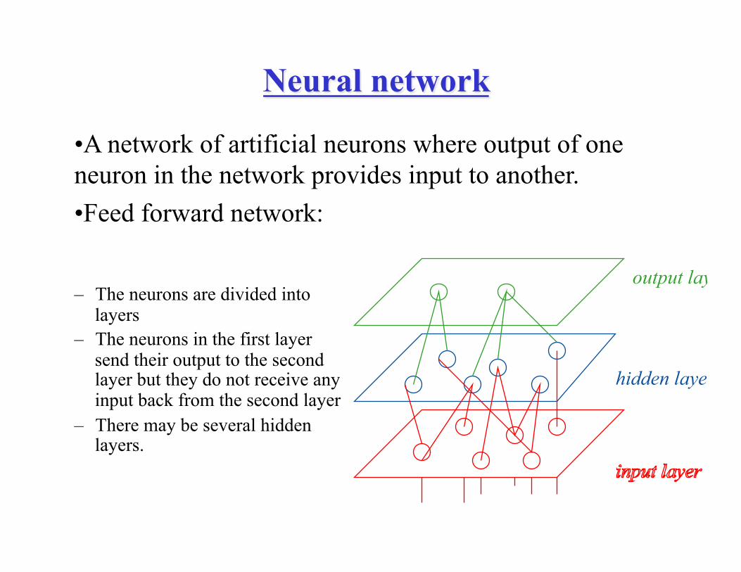
Neural network

–  The neurons are divided into

layers –  The neurons in the first layer

send their output to the second layer but they do not receive any input back from the second layer

–  There may be several hidden layers.

hidden layer

output layer

• A network of artificial neurons where output of one neuron in the network provides input to another. • Feed forward network:

Computing within NN

•  Each unit (except for input) computes weighted sums with weights selected during the training process.

•  Training – note that changing output in one units results in a different input to another unit. Training method – backpropagation “pushing the error towards input nodes”

PHD – neural network algorithm for secondary structure prediction

Rost and Sander

•  First step – multiple alignment (say for the sequence family recovered by BLAST)

•  PHD uses two levels of Neural Networks •  Level 1: Sequence to structure network: feed forward

NN with 3 layers – input, hidden, output; responsible for scoring chances of residuum to be in any of the three secondary structures based on the residuum and its sequence neighbors (like GOR but using MSA(!) and Neural Nets)

•  Level 2: Structure to structure network: arithmetic averaging over independently trained networks.

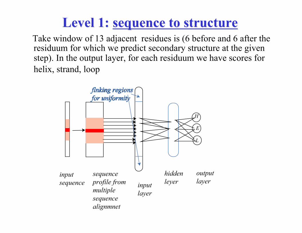
Level 1: sequence to structure Take window of 13 adjacent residues is (6 before and 6 after the

residuum for which we predict secondary structure at the given step). In the output layer, for each residuum we have scores for helix, strand, loop

inputsequence

sequenceprofile frommultiplesequencealignmnet

inputlayer

hiddenleyer

H

E

L

outputlayer

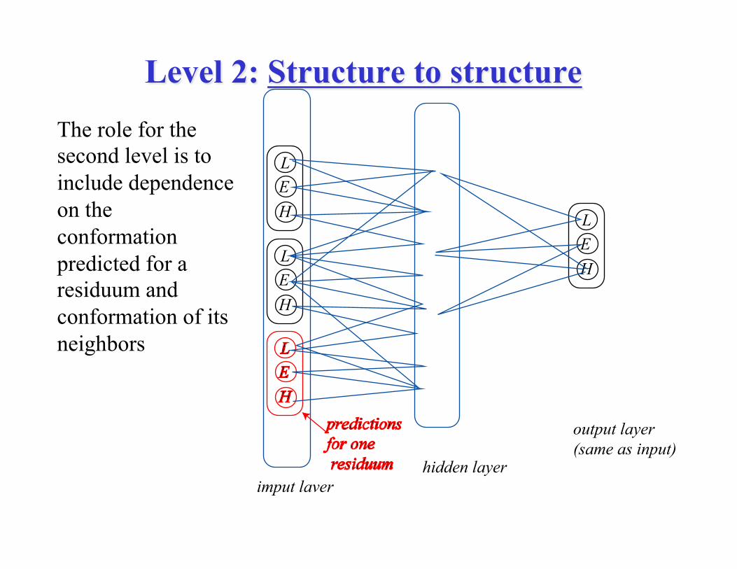
Level 2: Structure to structure The role for the second level is to include dependence on the conformation predicted for a residuum and conformation of its neighbors

HEL

HEL

HEL

imput laver

output layer(same as input)

hidden layer

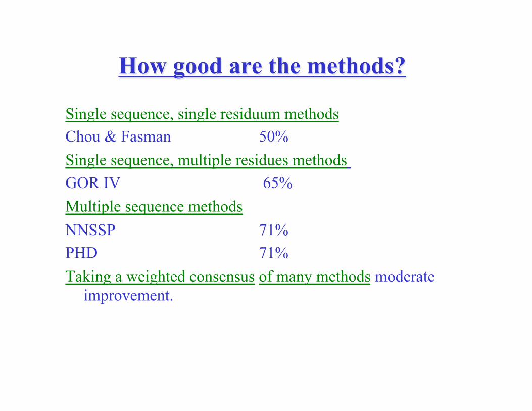
How good are the methods?

Single sequence, single residuum methods Chou & Fasman 50% Single sequence, multiple residues methods GOR IV 65% Multiple sequence methods NNSSP 71% PHD 71% Taking a weighted consensus of many methods moderate

improvement.