1

Lecture #2Planetary Wave Models

Charles McLandress (Banff Summer School 7-13 May 2005)

2

Outline of Lecture

1. Observational motivation2. Forced planetary waves in the

stratosphere3. Traveling planetary waves in the

mesosphere (the 2-day wave)

3

Part 1: ObservationalMotivation

4

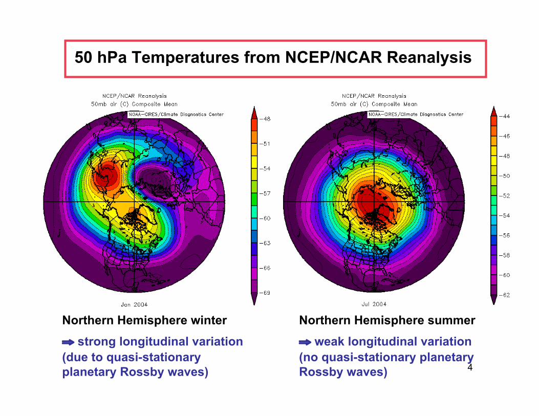
Northern Hemisphere winter⇒ strong longitudinal variation(due to quasi-stationaryplanetary Rossby waves)

Northern Hemisphere summer⇒ weak longitudinal variation(no quasi-stationary planetaryRossby waves)

50 hPa Temperatures from NCEP/NCAR Reanalysis

5

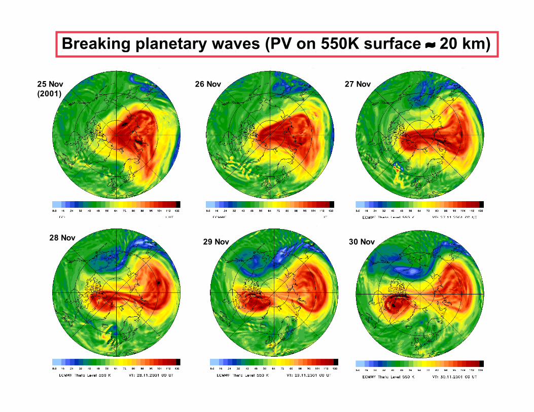
Breaking planetary waves (PV on 550K surface ≈ 20 km)

25 Nov(2001)

26 Nov 27 Nov

28 Nov 29 Nov 30 Nov

6

NP

SP

φ

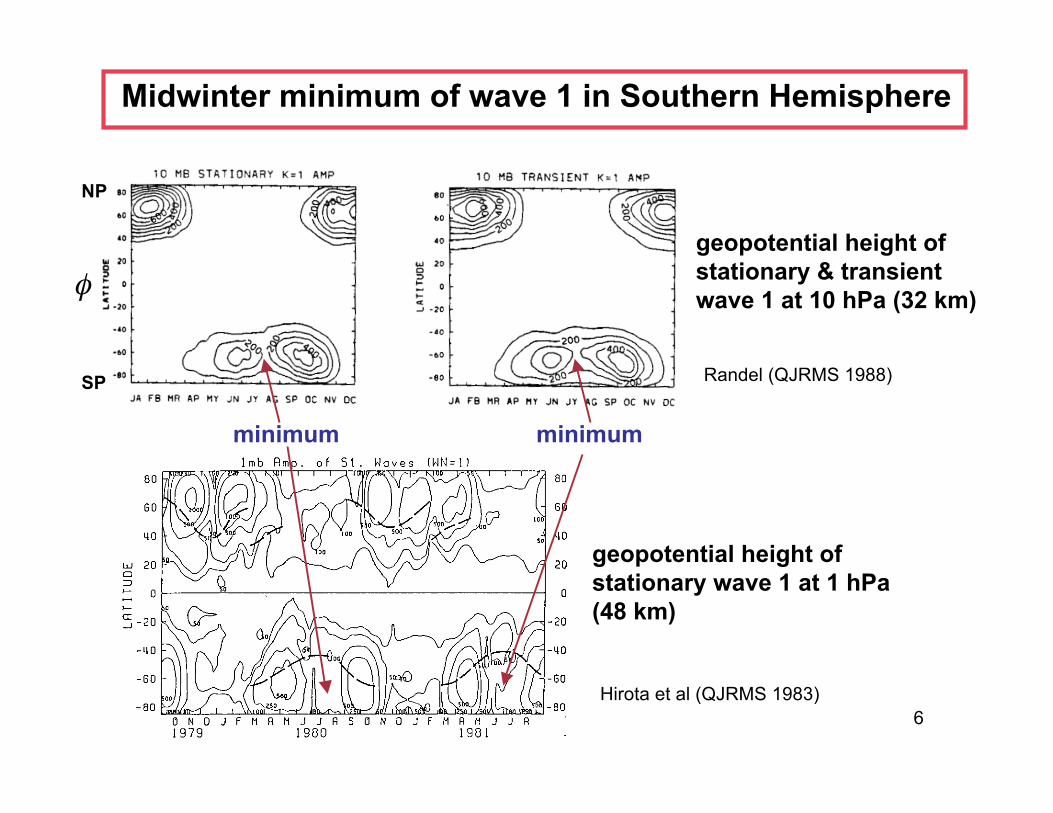
minimum minimum

Midwinter minimum of wave 1 in Southern Hemisphere

Randel (QJRMS 1988)

Hirota et al (QJRMS 1983)

geopotential height ofstationary wave 1 at 1 hPa(48 km)

geopotential height ofstationary & transientwave 1 at 10 hPa (32 km)

7

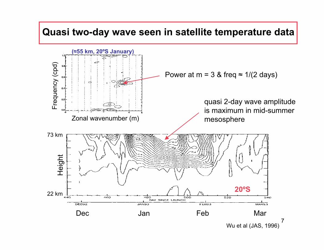
Quasi two-day wave seen in satellite temperature data

Power at m = 3 & freq ≈ 1/(2 days)

Zonal wavenumber (m)

Freq

uenc

y (c

pd)

quasi 2-day wave amplitudeis maximum in mid-summermesosphere

Dec MarJan Feb

20ºS

Hei

ght

73 km

22 km

Wu et al (JAS, 1996)

(≈55 km, 20ºS January)

8

Part 2: Forced planetarywaves in the stratosphere

9

Characteristics of planetary Rossby waves

• planetary waves are disturbances having zonalwavelengths of the scale of the earth’s radius.

• PWs in extratropics are in approximate geostrophicbalance (referred to as planetary Rossby waves).

• forced in the troposphere by topography, land-seatemperature contrasts, and synoptic eddies.

• restoring force is latitudinal gradient of background PV.• horizontal propagation is westward with respect to the

background zonal wind.• vertical propagation into the stratosphere occurs for the

longest spatial scales.

10

PW Models to be discussed

1. Barotropic model on the β-plane2. Linear quasi-geostrophic model on

the β-plane3. Linear quasi-geostrophic model on

the sphere4. Quasi-linear models

11

1. Barotropic PW modelon the β-plane

• incompressible fluid with purely horizontal flow.• Newton’s laws results in two equations for the

zonal and meridional wind components.• these two equations can be combined to form

the vorticity equation.• further simplification is made by replacing the

spherical geometry with Cartesian geometryand by writing the Coriolis parameter f = 2Ωsinφ= fo+βy (the β-plane approximation).

12

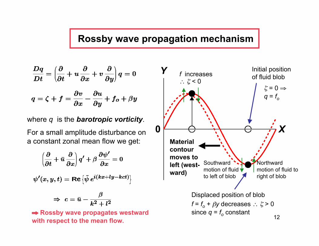
where q is the barotropic vorticity.

For a small amplitude disturbance ona constant zonal mean flow we get:

Rossby wave propagation mechanism

X

Y Initial positionof fluid blob

0

ζ = 0 ⇒q = fo

Displaced position of blobf = fo + βy decreases ∴ ζ > 0since q = fo constant

Northwardmotion of fluid toright of blob

Southwardmotion of fluidto left of blob

Materialcontourmoves toleft (west-ward)

f increases∴ ζ < 0

⇒ Rossby wave propagates westwardwith respect to the mean flow.

13

2. Linear quasi-geostrophic PWmodel on the β-plane

• governing equations are:– equations of motion for the horizontal winds– hydrostatic equation– thermodynamic equation– mass continuity equation

• combined into a single equation called the quasi-geostrophic potential vorticity equation.

• Cartesian geometry simplifies the problem.• β-plane approximation is employed to retain the

latitudinal gradient of the planetary vorticity.

14

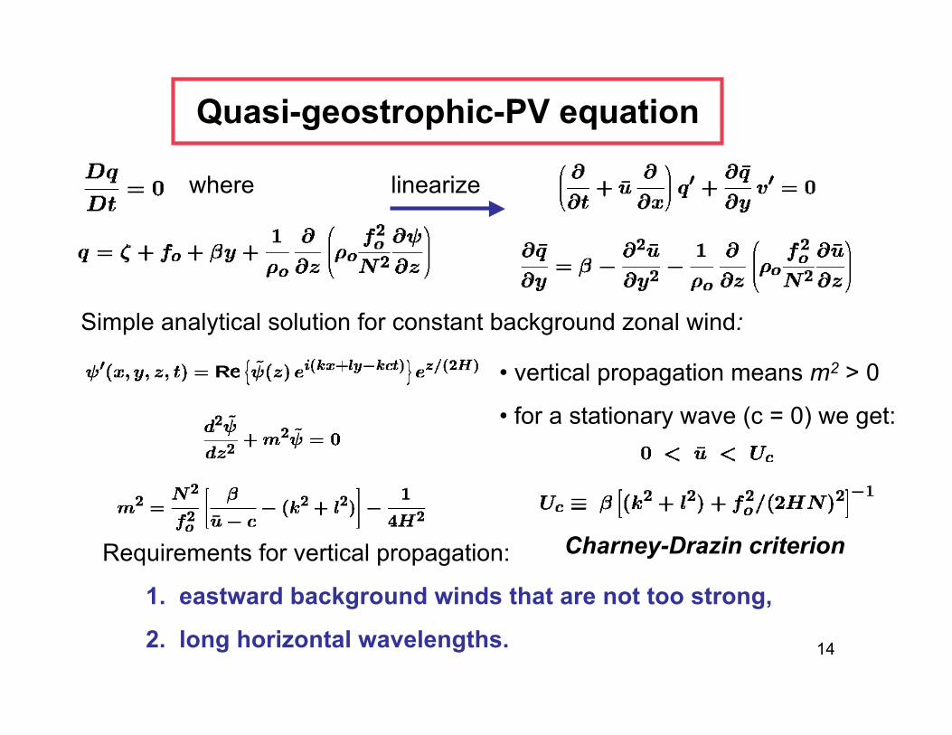
Quasi-geostrophic-PV equation

linearize

• vertical propagation means m2 > 0

• for a stationary wave (c = 0) we get:

Requirements for vertical propagation:

1. eastward background winds that are not too strong,

2. long horizontal wavelengths.

Charney-Drazin criterion

where

Simple analytical solution for constant background zonal wind:

15

3. Linear quasi-geostrophic PWmodel on the sphere

• quasi-geostrophic potential vorticity equationon the sphere

• stationary waves• examines impact of latitudinal and vertical

shear of background wind.• PW structure computed numerically.• Matsuno (JAS, 1970)

16

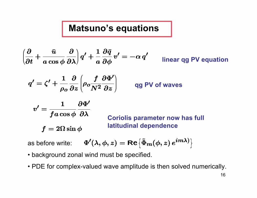
Matsuno’s equations

linear qg PV equation

qg PV of waves

as before write:

• background zonal wind must be specified.

• PDE for complex-valued wave amplitude is then solved numerically.

Coriolis parameter now has fulllatitudinal dependence

17

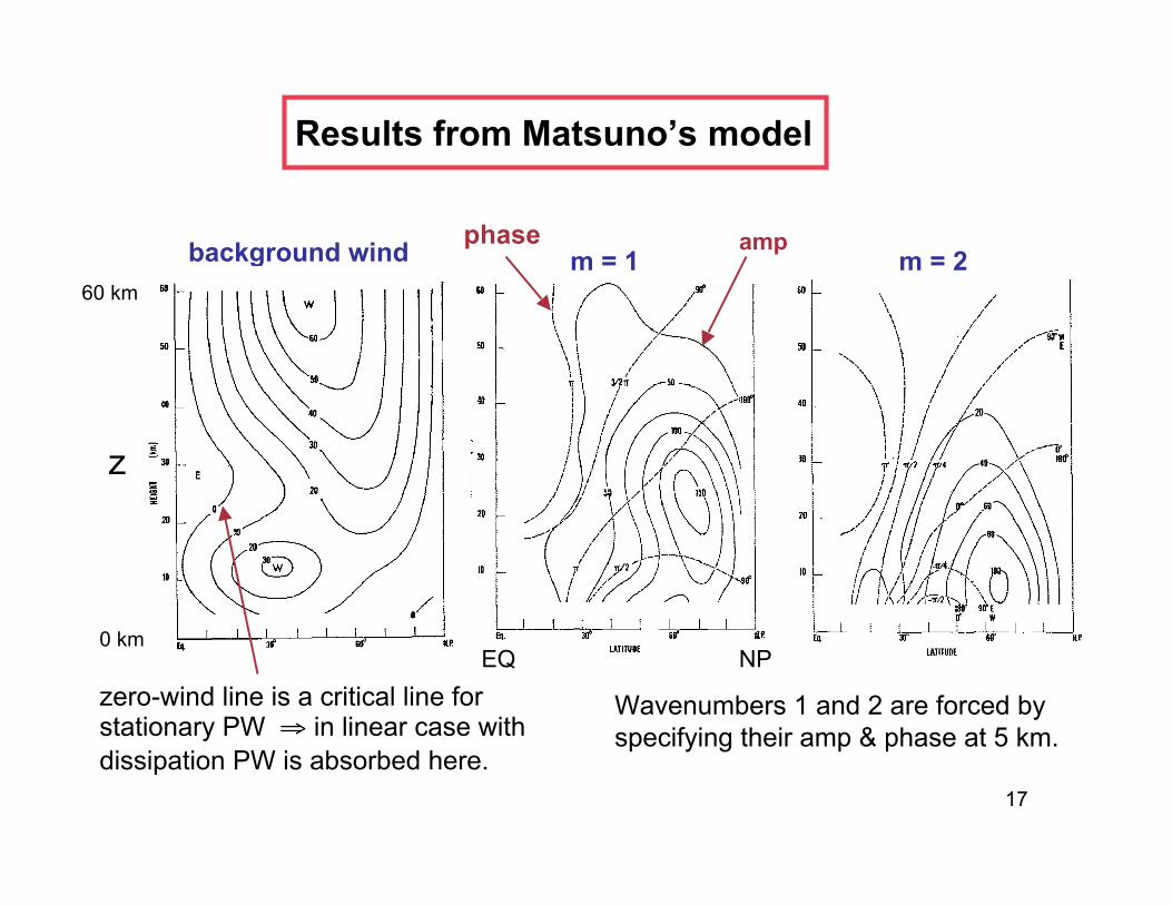
Results from Matsuno’s model

zero-wind line is a critical line forstationary PW ⇒ in linear case withdissipation PW is absorbed here.

Wavenumbers 1 and 2 are forced byspecifying their amp & phase at 5 km.

background wind m = 1 m = 2

EQ NP

60 km

0 km

z

ampphase

18

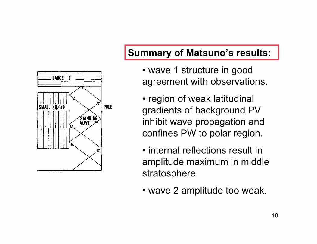
Summary of Matsuno’s results:

• wave 1 structure in goodagreement with observations.

• region of weak latitudinalgradients of background PVinhibit wave propagation andconfines PW to polar region.

• internal reflections result inamplitude maximum in middlestratosphere.

• wave 2 amplitude too weak.

19

4. Quasi-linear PW models

• planetary Rossby waves break in the stratosphere andinteract strongly with the zonal mean flow.

• here we discuss several models which allow for thisinteraction but use only a single zonal wavenumber.

• referred to as quasi-linear because the wave caninteract with the zonal mean flow but not with itself.

• validity of quasi-linear models was demonstrated byHaynes & McIntyre (1987) in context of barotropic model.

• we will use these models to try to explain the mid-winterminimum in PW 1 amplitude in the SH.

20

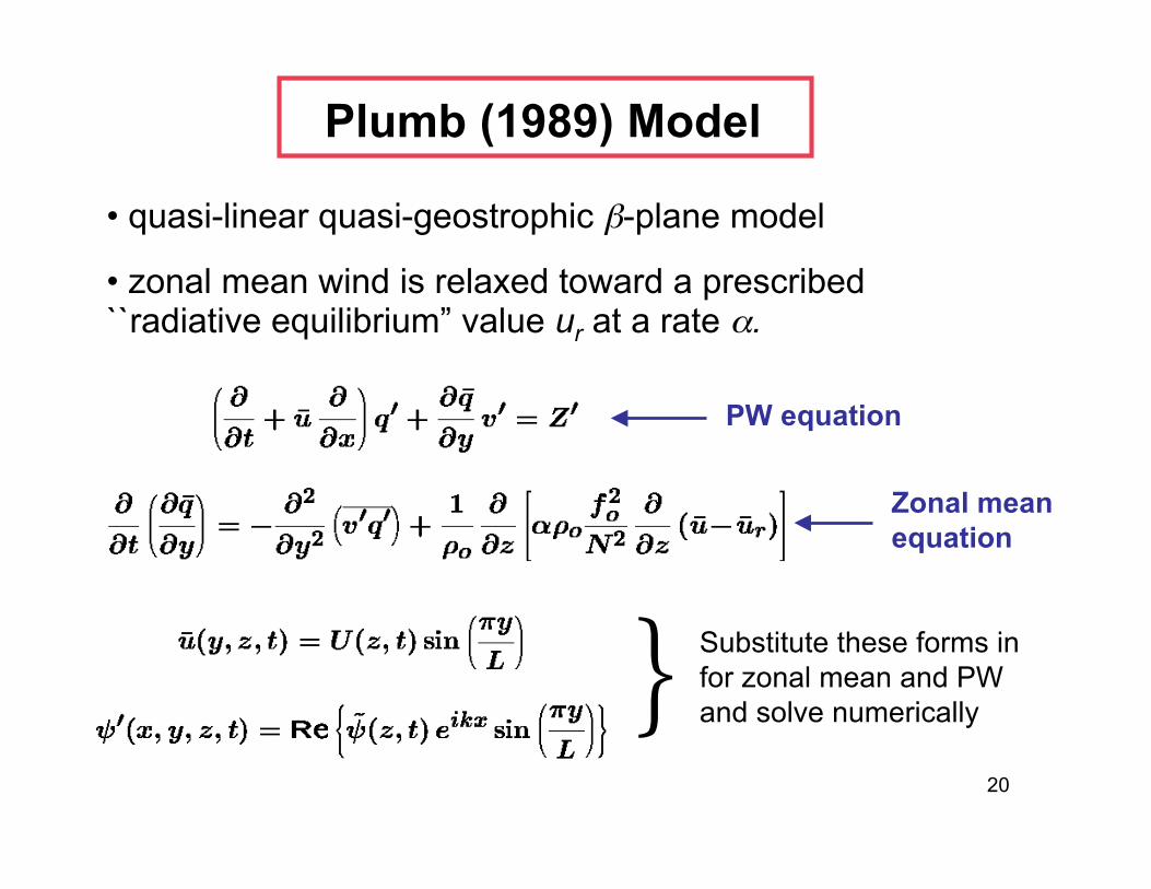
Plumb (1989) Model

• quasi-linear quasi-geostrophic β-plane model

• zonal mean wind is relaxed toward a prescribed``radiative equilibrium” value ur at a rate α.

PW equation

Zonal meanequation

!

Substitute these forms infor zonal mean and PWand solve numerically

21

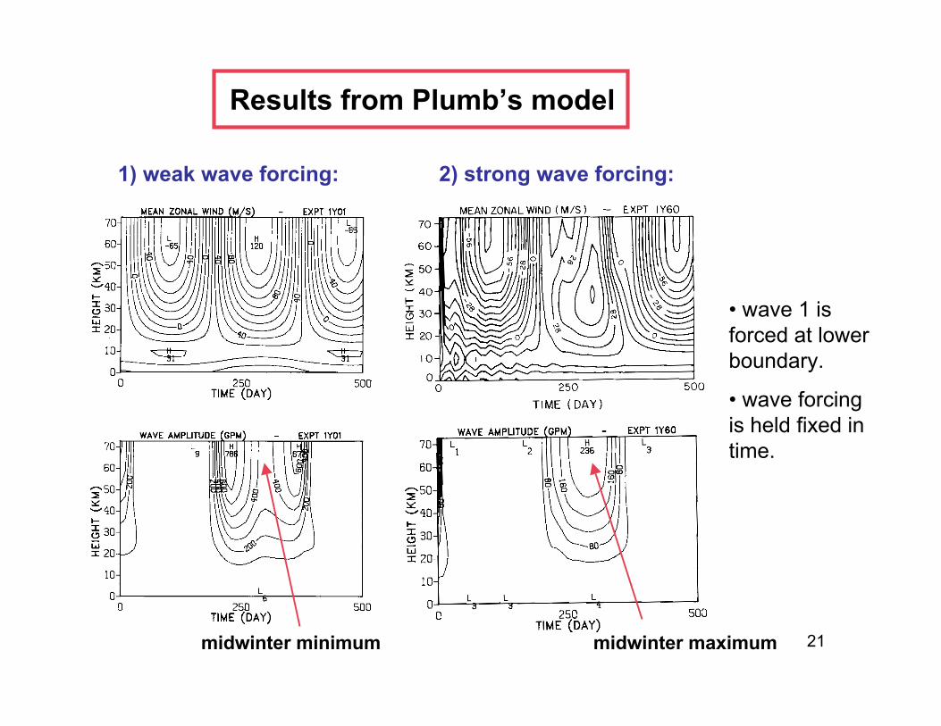
Results from Plumb’s model

1) weak wave forcing: 2) strong wave forcing:

midwinter minimum midwinter maximum

• wave 1 isforced at lowerboundary.

• wave forcingis held fixed intime.

22

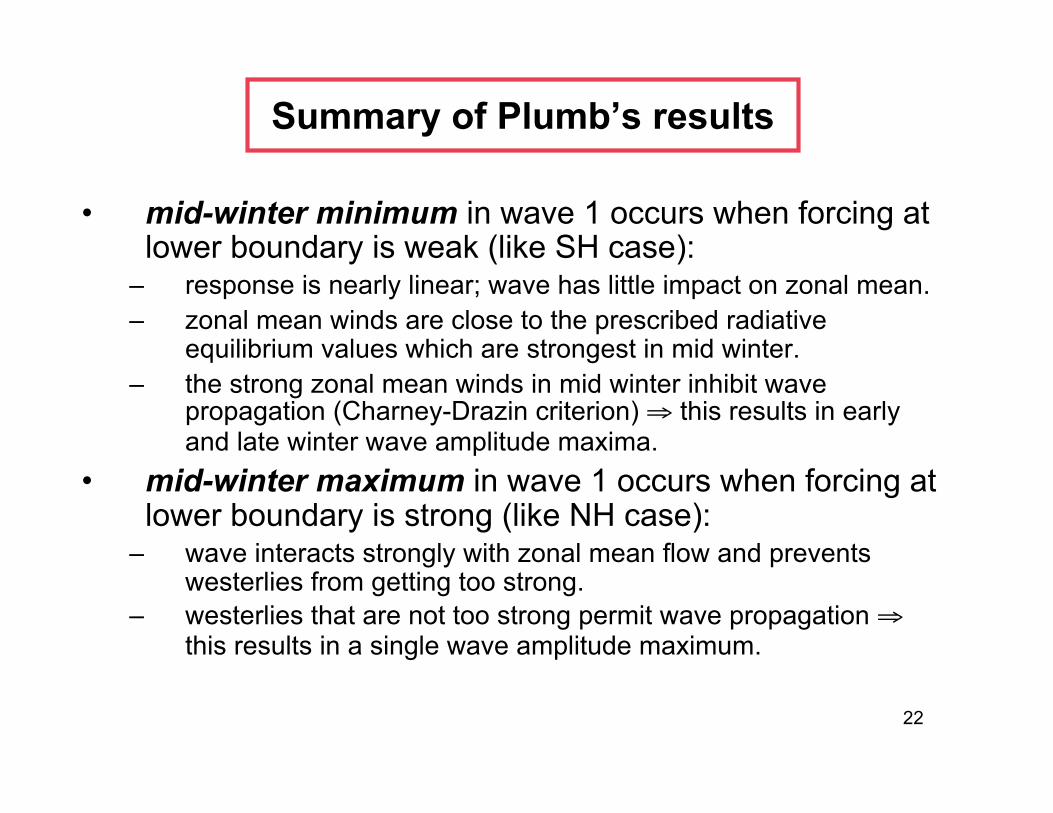
Summary of Plumb’s results

• mid-winter minimum in wave 1 occurs when forcing atlower boundary is weak (like SH case):

– response is nearly linear; wave has little impact on zonal mean.– zonal mean winds are close to the prescribed radiative

equilibrium values which are strongest in mid winter.– the strong zonal mean winds in mid winter inhibit wave

propagation (Charney-Drazin criterion) ⇒ this results in earlyand late winter wave amplitude maxima.

• mid-winter maximum in wave 1 occurs when forcing atlower boundary is strong (like NH case):

– wave interacts strongly with zonal mean flow and preventswesterlies from getting too strong.

– westerlies that are not too strong permit wave propagation ⇒this results in a single wave amplitude maximum.

23

Some weaknesses of Plumb’s model

• Latitudinal propagation of waves not considered.• Impact of latitudinal shear in zonal mean wind (i.e.,

latitudinal gradients of zonal mean PV) notconsidered.

24

Mechanistic primitive equation PW model

• Scott and Haynes (JAS, 2002)• primitive equations on the sphere• stratosphere-only model• single stationary PW is forced at the lower

boundary which is at 100 hPa.• seasonal cycle is included by thermal relaxation

to a seasonally varying temperature field.• importance of latitudinal propagation can be

examined which was not possible with thePlumb model.

25

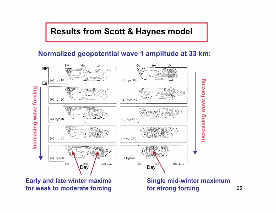
Results from Scott & Haynes model

Early and late winter maximafor weak to moderate forcing

Single mid-winter maximumfor strong forcing

NP

Eq

Incr

easi

ng w

ave

forc

ing

Incr

easi

ng w

ave

forc

ing

Normalized geopotential wave 1 amplitude at 33 km:

DayDay

26

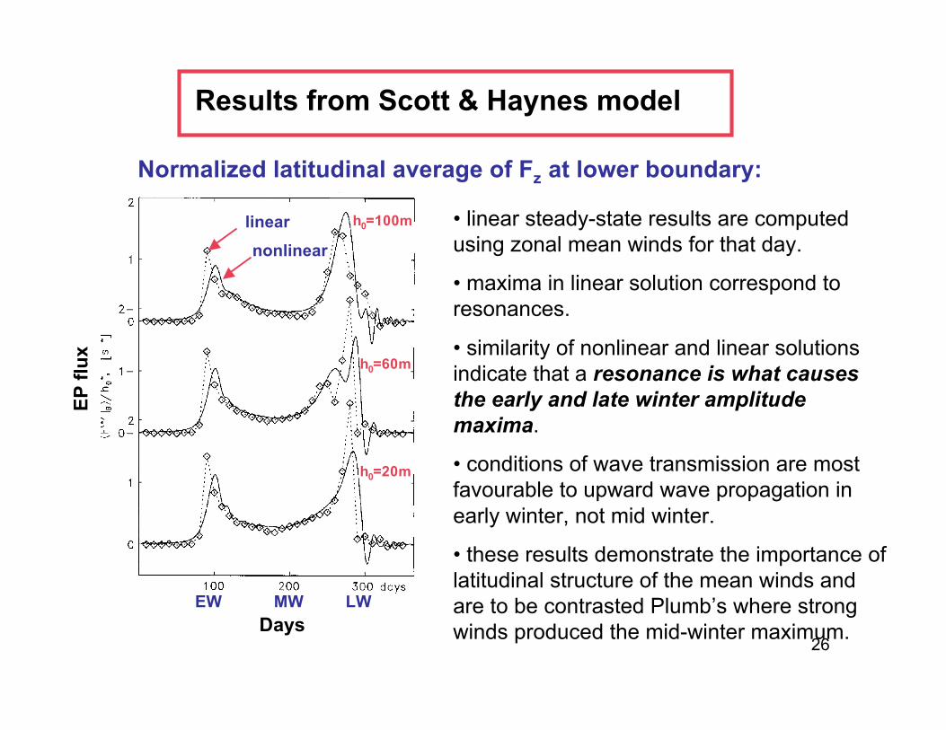
Results from Scott & Haynes model

linearnonlinear

EW MW LW Days

EP fl

ux

h0=100m

h0=60m

h0=20m

• linear steady-state results are computedusing zonal mean winds for that day.

• maxima in linear solution correspond toresonances.

• similarity of nonlinear and linear solutionsindicate that a resonance is what causesthe early and late winter amplitudemaxima.

• conditions of wave transmission are mostfavourable to upward wave propagation inearly winter, not mid winter.

• these results demonstrate the importance oflatitudinal structure of the mean winds andare to be contrasted Plumb’s where strongwinds produced the mid-winter maximum.

Normalized latitudinal average of Fz at lower boundary:

27

Part 3: Traveling planetarywaves in the mesosphere

(the 2-day wave)

28

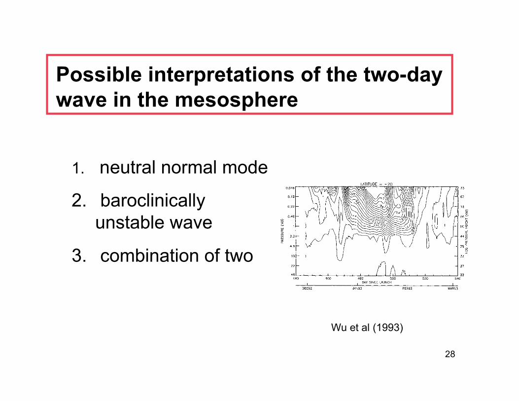
Possible interpretations of the two-daywave in the mesosphere

1. neutral normal mode

2. baroclinicallyunstable wave

3. combination of two

Wu et al (1993)

29

Models described here to study 2-day wave

1. a linear 2D (latitude by height) primitiveequations model where wave frequencyand zonal wavenumber are specified

2. 3D middle atmosphere GCM

30

Neutral Normal Modes

• normal modes of the atmosphere are free (unforced)disturbances.

• neutral means that the frequency is real-valued (i.e., notexponentially growing or decaying).

• analytical solutions are obtained by solving the linearprimitive equations on the sphere for a windlessbackground atmosphere without dissipation.

• for each zonal wavenumber there is a discrete set ofnormal modes each with a different frequency andmeridional structure.

• if a disturbance is forced at this frequency the responseis resonant ⇒ it is the normal mode that grows mostrapidly in time and dominates the overall response.

31

2.1 2.3Period (days)

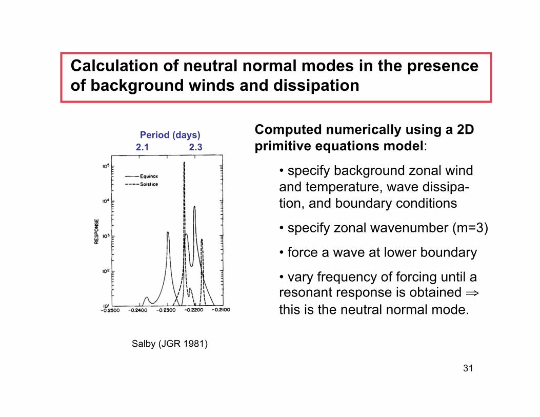
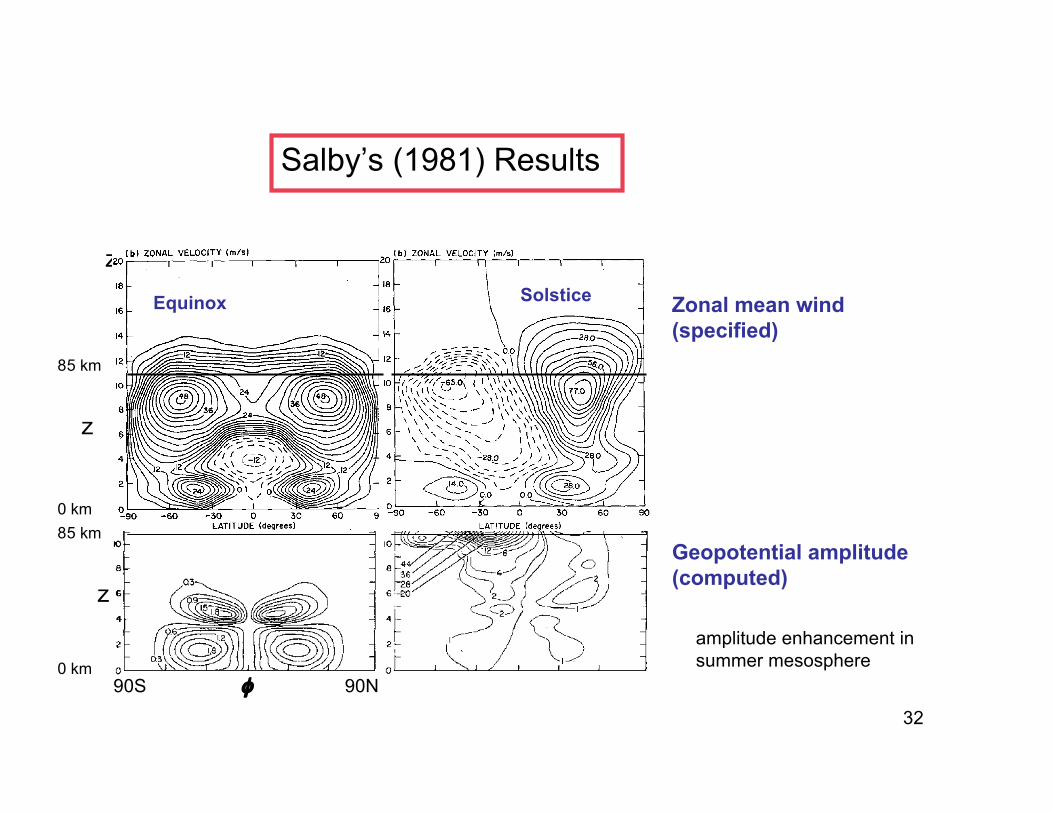
Calculation of neutral normal modes in the presenceof background winds and dissipation

Salby (JGR 1981)

Computed numerically using a 2Dprimitive equations model:

• specify background zonal windand temperature, wave dissipa-tion, and boundary conditions

• specify zonal wavenumber (m=3)

• force a wave at lower boundary

• vary frequency of forcing until aresonant response is obtained ⇒this is the neutral normal mode.

32

z

Zonal mean wind(specified)

Geopotential amplitude(computed)

Salby’s (1981) Results

amplitude enhancement insummer mesosphere

Equinox Solstice

z

z

90S 90Nφ

85 km

85 km0 km

0 km

33

Instability mechanism ofthe two-day wave

• proposed by Plumb (1983)• zonal mean easterlies near solstice may

be baroclinically unstable.• simulations using middle atmosphere

GCMs reveal that 2-day waveamplification is related to baroclinic andbarotropic instability of zonal mean state.

34

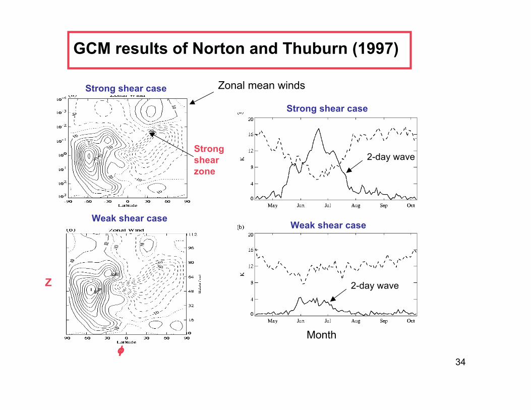
Strong shear case

Weak shear case

Strong shear case

Weak shear case

2-day wave

2-day wave

Month

GCM results of Norton and Thuburn (1997)

φ

Z

Zonal mean winds

Strongshearzone

35

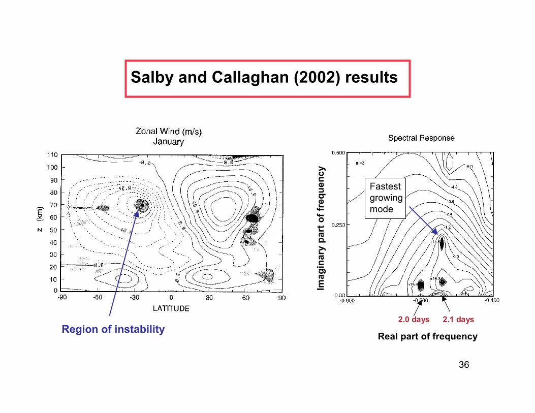
• the relationship between neutral normal modesand instability were examined by Salby andCallaghan (JAS 2002).

• they used Salby’s (1981) 2D primitiveequations model but considered unstable zonalmean background states and computed normalmodes for complex-valued frequencies.

⇒ positive imaginary frequencies indicateexponential wave growth.

Normal Modes in an unstable mean flow

36

Salby and Callaghan (2002) results

Region of instabilityIm

agin

ary

part

of f

requ

ency

Real part of frequency

Fastestgrowingmode

2.0 days 2.1 days

37

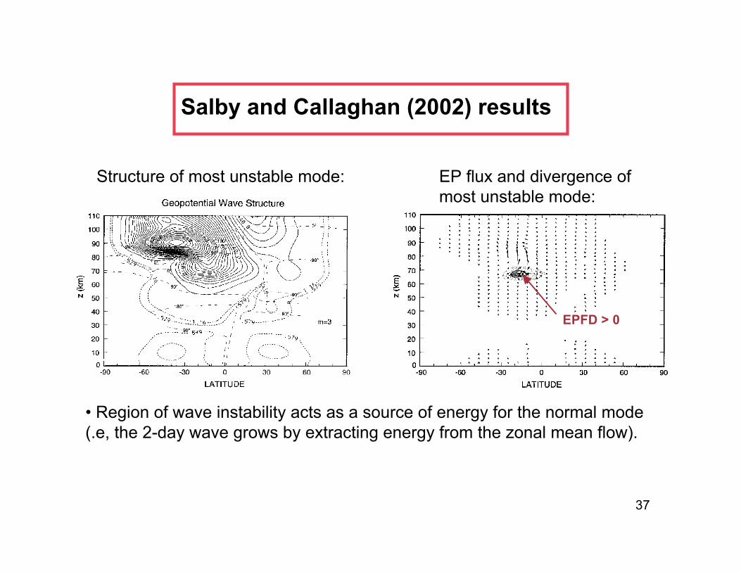
Salby and Callaghan (2002) results

Structure of most unstable mode: EP flux and divergence ofmost unstable mode:

EPFD > 0

• Region of wave instability acts as a source of energy for the normal mode(.e, the 2-day wave grows by extracting energy from the zonal mean flow).

38

Summary of 2-day wave results

• The two opposing interpretations of the 2-daywave (neutral normal mode vs instability)now appear to be reconciled. Hurrah.– instability of the background state generates

unstable normal modes that grow in time.– real part of the frequency and spatial structure of

the most unstable mode is in good agreementwith the observed 2-day wave.

39

The End