Lecture 2: It Calculus and Stochastic Differential Equationsssarkka/course_s2012/pdf/handout2.pdf · differential equations of the form dx dt = f(x,t) +L(x,t)w(t), For linear equations

Lecture 2: Itô Calculus and Stochastic Differential

Equations

Simo Särkkä

Aalto UniversityTampere University of Technology

Lappeenranta University of TechnologyFinland

November 1, 2012

Simo Särkkä (Aalto/TUT/LUT) Lecture 2: Itô Calculus and SDEs November 1, 2012 1 / 34

Contents

1 Introduction

2 Stochastic integral of Itô

3 Itô formula

4 Solutions of linear SDEs

5 Non-linear SDE, solution existence, etc.

6 Summary


SDEs as white noise driven differential equations

During the last lecture we treated SDEs as white-noise driven

differential equations of the form

dx

dt= f(x, t) + L(x, t)w(t),

For linear equations the approach worked ok.

But there is something strange going on:

The usage of chain rule of calculus led to wrong results.

With non-linear differential equations we were completely lost.Picard-Lindelöf theorem did not work at all.

The source of all the problems is the everywhere discontinuous

white noise w(t).

So how should we really formulate SDEs?


Equivalent integral equation

Integrating the differential equation from t0 to t gives:

x(t)− x(t0) =

∫ t

t0

f(x(t), t) dt +

∫ t

t0

L(x(t), t)w(t) dt .

The first integral is just a normal Riemann/Lebesgue integral.

The second integral is the problematic one due to the white noise.

This integral cannot be defined as Riemann, Stieltjes or Lebesgue

integral as we shall see next.


Attempt 1: Riemann integral

In the Riemannian sense the integral would be defined as

∫ t

t0

L(x(t), t)w(t) dt = limn→∞

∑

k

L(x(t∗k ), t∗

k )w(t∗k ) (tk+1 − tk ),

where t0 < t1 < . . . < tn = t and t∗k ∈ [tk , tk+1].

Upper and lower sums are defined as the selections of t∗k such

that the integrand L(x(t∗k ), t∗

k )w(t∗k ) has its maximum and

minimum values, respectively.

The Riemann integral exists if the upper and lower sums converge

to the same value.

Because white noise is discontinuous everywhere, the Riemann

integral does not exist.


Attempt 2: Stieltjes integral

Stieltjes integral is more general than the Riemann integral.

In particular, it allows for discontinuous integrands.

We can interpret the increment w(t) dt as increment of another

process β(t) such that

∫ t

t0

L(x(t), t)w(t) dt =

∫ t

t0

L(x(t), t) dβ(t).

It turns out that a suitable process for this purpose is the Brownian

motion —


Brownian motion

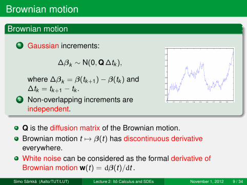
Brownian motion

1 Gaussian increments:

∆βk ∼ N(0,Q∆tk ),

where ∆βk = β(tk+1)− β(tk ) and

∆tk = tk+1 − tk .

2 Non-overlapping increments are

independent.0 0.1 0.2 0.3 0.4 0.5 0.6 0.7 0.8 0.9 1

0

0.2

0.4

0.6

0.8

1

1.2

1.4

1.6

1.8

Q is the diffusion matrix of the Brownian motion.

Brownian motion t 7→ β(t) has discontinuous derivative

everywhere.

White noise can be considered as the formal derivative of

Brownian motion w(t) = dβ(t)/dt .


Attempt 2: Stieltjes integral (cont.)

Stieltjes integral is defined as a limit of the form

∫ t

t0

L(x(t), t) dβ = limn→∞

∑

k

L(x(t∗k ), t∗

k ) [β(tk+1)− β(tk )],

where t0 < t1 < . . . < tn and t∗k ∈ [tk , tk+1].

The limit t∗k should be independent of the position on the interval

t∗k ∈ [tk , tk+1].

But for integration with respect to Brownian motion this is not the

case.

Thus, Stieltjes integral definition does not work either.


Attempt 3: Lebesgue integral

In Lebesgue integral we could interpret β(t) to define a “stochastic

measure” via β((u, v)) = β(u)− β(v).

Essentially, this will also lead to the definition

∫ t

t0

L(x(t), t) dβ = limn→∞

∑

k

L(x(t∗k ), t∗

k ) [β(tk+1)− β(tk )],

where t0 < t1 < . . . < tn and t∗k ∈ [tk , tk+1].

Again, the limit should be independent of the choice t∗k ∈ [tk , tk+1].

Also our “measure” is not really a sensible measure at all.

⇒ Lebesgue integral does not work either.


Attempt 4: Itô integral

The solution to the problem is the Itô stochastic integral.

The idea is to fix the choice to t∗k = tk , and define the integral as

∫ t

t0

L(x(t), t) dβ(t) = limn→∞

∑

k

L(x(tk ), tk ) [β(tk+1)− β(tk )].

This Itô stochastic integral turns out to be a sensible definition of

the integral.

However, the resulting integral does not obey the computational

rules of ordinary calculus.

Instead of ordinary calculus we have Itô calculus.


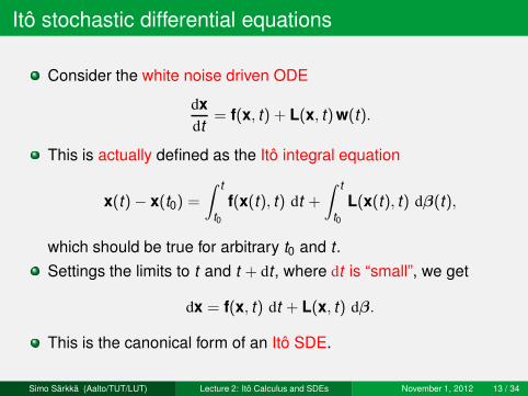
Itô stochastic differential equations

Consider the white noise driven ODE

dx

dt= f(x, t) + L(x, t)w(t).

This is actually defined as the Itô integral equation

x(t)− x(t0) =

∫ t

t0

f(x(t), t) dt +

∫ t

t0

L(x(t), t) dβ(t),

which should be true for arbitrary t0 and t .

Settings the limits to t and t + dt , where dt is “small”, we get

dx = f(x, t) dt + L(x, t) dβ.

This is the canonical form of an Itô SDE.


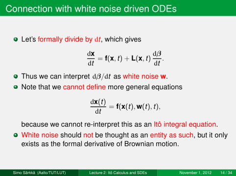
Connection with white noise driven ODEs

Let’s formally divide by dt , which gives

dx

dt= f(x, t) + L(x, t)

dβ

dt.

Thus we can interpret dβ/dt as white noise w.

Note that we cannot define more general equations

dx(t)

dt= f(x(t),w(t), t),

because we cannot re-interpret this as an Itô integral equation.

White noise should not be thought as an entity as such, but it only

exists as the formal derivative of Brownian motion.


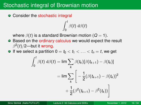
Stochastic integral of Brownian motion

Consider the stochastic integral∫ t

0

β(t) dβ(t)

where β(t) is a standard Brownian motion (Q = 1).

Based on the ordinary calculus we would expect the result

β2(t)/2—but it wrong.

If we select a partition 0 = t0 < t1 < . . . < tn = t , we get∫ t

0

β(t) dβ(t) = lim∑

k

β(tk )[β(tk+1)− β(tk )]

= lim∑

k

[

−1

2(β(tk+1)− β(tk ))

2

+1

2(β2(tk+1)− β2(tk ))

]


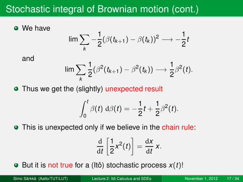
Stochastic integral of Brownian motion (cont.)

We have

lim∑

k

−1

2(β(tk+1)− β(tk ))

2−→ −

1

2t

and

lim∑

k

1

2(β2(tk+1)− β2(tk )) −→

1

2β2(t).

Thus we get the (slightly) unexpected result

∫ t

0

β(t) dβ(t) = −1

2t +

1

2β2(t).

This is unexpected only if we believe in the chain rule:

d

dt

[

1

2x2(t)

]

=dx

dtx .

But it is not true for a (Itô) stochastic process x(t)!


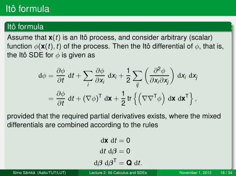
Itô formula

Itô formula

Assume that x(t) is an Itô process, and consider arbitrary (scalar)

function φ(x(t), t) of the process. Then the Itô differential of φ, that is,

the Itô SDE for φ is given as

dφ =∂φ

∂tdt +

∑

i

∂φ

∂xidxi +

1

2

∑

ij

(

∂2φ

∂xi∂xj

)

dxi dxj

=∂φ

∂tdt + (∇φ)T

dx +1

2tr{(

∇∇Tφ

)

dx dxT}

,

provided that the required partial derivatives exists, where the mixed

differentials are combined according to the rules

dx dt = 0

dt dβ = 0

dβ dβT = Q dt .


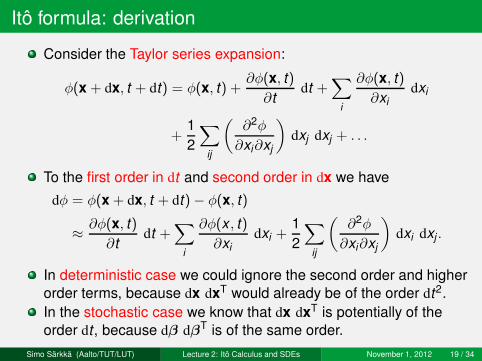
Itô formula: derivation

Consider the Taylor series expansion:

φ(x + dx, t + dt) = φ(x, t) +∂φ(x, t)

∂tdt +

∑

i

∂φ(x, t)

∂xidxi

+1

2

∑

ij

(

∂2φ

∂xi∂xj

)

dxj dxj + . . .

To the first order in dt and second order in dx we have

dφ = φ(x + dx, t + dt)− φ(x, t)

≈∂φ(x, t)

∂tdt +

∑

i

∂φ(x , t)

∂xidxi +

1

2

∑

ij

(

∂2φ

∂xi∂xj

)

dxi dxj .

In deterministic case we could ignore the second order and higher

order terms, because dx dxT would already be of the order dt2.

In the stochastic case we know that dx dxT is potentially of the

order dt , because dβ dβT is of the same order.


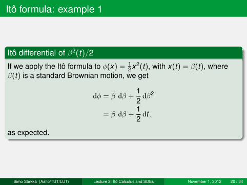
Itô formula: example 1

Itô differential of β2(t)/2

If we apply the Itô formula to φ(x) = 12x2(t), with x(t) = β(t), where

β(t) is a standard Brownian motion, we get

dφ = β dβ +1

2dβ2

= β dβ +1

2dt ,

as expected.


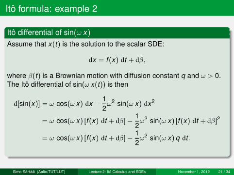
Itô formula: example 2

Itô differential of sin(ω x)

Assume that x(t) is the solution to the scalar SDE:

dx = f (x) dt + dβ,

where β(t) is a Brownian motion with diffusion constant q and ω > 0.

The Itô differential of sin(ω x(t)) is then

d[sin(x)] = ω cos(ω x) dx −1

2ω2 sin(ω x) dx2

= ω cos(ω x) [f (x) dt + dβ]−1

2ω2 sin(ω x) [f (x) dt + dβ]2

= ω cos(ω x) [f (x) dt + dβ]−1

2ω2 sin(ω x)q dt .


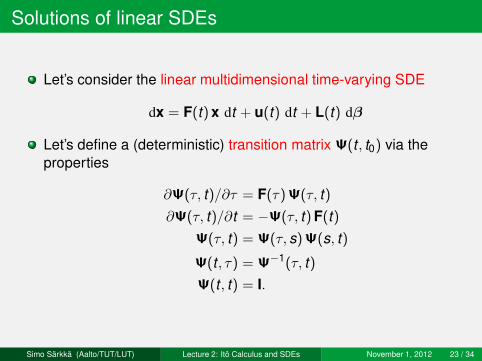
Solutions of linear SDEs

Let’s consider the linear multidimensional time-varying SDE

dx = F(t)x dt + u(t) dt + L(t) dβ

Let’s define a (deterministic) transition matrix Ψ(t , t0) via the

properties

∂Ψ(τ, t)/∂τ = F(τ)Ψ(τ, t)

∂Ψ(τ, t)/∂t = −Ψ(τ, t)F(t)

Ψ(τ, t) = Ψ(τ, s)Ψ(s, t)

Ψ(t , τ) = Ψ−1(τ, t)

Ψ(t , t) = I.


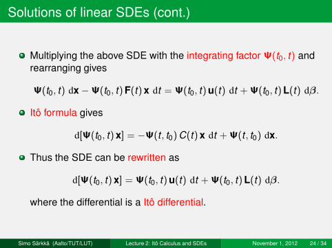
Solutions of linear SDEs (cont.)

Multiplying the above SDE with the integrating factor Ψ(t0, t) and

rearranging gives

Ψ(t0, t) dx −Ψ(t0, t)F(t)x dt = Ψ(t0, t)u(t) dt +Ψ(t0, t)L(t) dβ.

Itô formula gives

d[Ψ(t0, t)x] = −Ψ(t , t0)C(t)x dt +Ψ(t , t0) dx.

Thus the SDE can be rewritten as

d[Ψ(t0, t)x] = Ψ(t0, t)u(t) dt +Ψ(t0, t)L(t) dβ.

where the differential is a Itô differential.


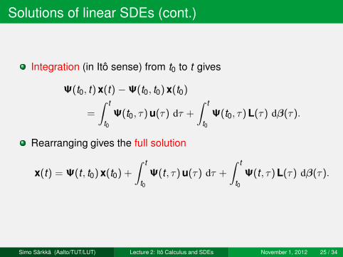
Solutions of linear SDEs (cont.)

Integration (in Itô sense) from t0 to t gives

Ψ(t0, t)x(t) −Ψ(t0, t0)x(t0)

=

∫ t

t0

Ψ(t0, τ)u(τ) dτ +

∫ t

t0

Ψ(t0, τ)L(τ) dβ(τ).

Rearranging gives the full solution

x(t) = Ψ(t , t0)x(t0) +

∫ t

t0

Ψ(t , τ)u(τ) dτ +

∫ t

t0

Ψ(t , τ)L(τ) dβ(τ).


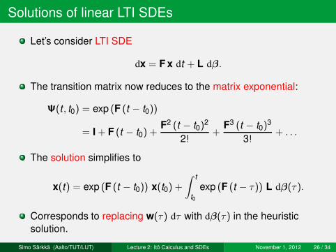
Solutions of linear LTI SDEs

Let’s consider LTI SDE

dx = F x dt + L dβ.

The transition matrix now reduces to the matrix exponential:

Ψ(t , t0) = exp (F (t − t0))

= I + F (t − t0) +F2 (t − t0)

2

2!+

F3 (t − t0)3

3!+ . . .

The solution simplifies to

x(t) = exp (F (t − t0)) x(t0) +

∫ t

t0

exp (F (t − τ)) L dβ(τ).

Corresponds to replacing w(τ) dτ with dβ(τ) in the heuristic

solution.


Solutions of linear LTI SDEs

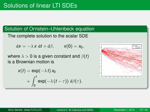
Solution of Ornstein–Uhlenbeck equation

The complete solution to the scalar SDE

dx = −λ x dt + dβ, x(0) = x0,

where λ > 0 is a given constant and β(t)is a Brownian motion is

x(t) = exp(−λ t) x0

+

∫ t

0

exp(−λ (t − τ)) dβ(τ).0 0.1 0.2 0.3 0.4 0.5 0.6 0.7 0.8 0.9 1

0

0.5

1

1.5

2

2.5

3

3.5

4

4.5

5

Mean95% quantilesRealizations


Non-linear SDEs

There is no general solution method for non-linear SDEs

dx = f(x, t) dt + L(x, t) dβ.

Sometimes we can use transformation/other methods from

deterministic setting and replace chain rule with Itô formula.

However, we can still use the Euler–Maruyama method presented

last time:

x̂(tk+1) = x̂(tk ) + f(x̂(tk ), tk )∆t + L(x̂(tk ), tk )∆βk ,

where ∆βk ∼ N(0,Q∆t).

The method might now look more natural, because ∆βk is just a

finite increment of Brownian motion.


Existence and uniqueness of solutions

The existence and uniqueness conditions for SDE solutions can

be proved via stochastic Picard iteration:

ϕ0(t) = x0

ϕn+1(t) = x0 +

∫ t

t0

f(ϕn(τ), τ) dτ +

∫ t

t0

L(ϕn(τ), τ) dβ(τ).

The iteration converges and thus the SDE has unique strongsolution provided that the following are met:

Functions f and L grow at most linearly in x.

Functions f and L are Lipschitz continuous in x.

A strong solution means a solution x for a given β — strong

uniqueness implies that the whole path is unique.

We can also have a weak solution which is some pair (x̃, β̃) which

solves the SDE.

Weak uniqueness means that the distribution is unique.


Stratonovich calculus

The symmetrized stochastic integral or the Stratonovich integral

can be defined as follows:

∫ t

t0

L(x(t), t) ◦ dβ(t) = limn→∞

∑

k

L(x(t∗k ), t∗

k ) [β(tk+1)− β(tk )],

where t∗k = (tk + tk )/2 is the midpoint.

Recall that in Itô integral we had the starting point t∗k = tk .

Now the Itô formula reduces to the rule from ordinary calculus.

Stratonovich integral is not a martingale which makes its

theoretical analysis harder.

Smooth approximations to white noise converge to the

Stratonovich integral.


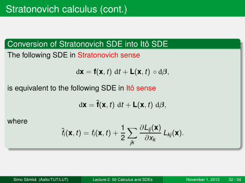
Stratonovich calculus (cont.)

Conversion of Stratonovich SDE into Itô SDE

The following SDE in Stratonovich sense

dx = f(x, t) dt + L(x, t) ◦ dβ,

is equivalent to the following SDE in Itô sense

dx = f̃(x, t) dt + L(x, t) dβ,

where

f̃i(x, t) = fi(x, t) +1

2

∑

jk

∂Lij(x)

∂xkLkj(x).


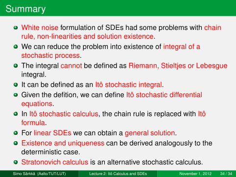
Summary

White noise formulation of SDEs had some problems with chain

rule, non-linearities and solution existence.

We can reduce the problem into existence of integral of a

stochastic process.

The integral cannot be defined as Riemann, Stieltjes or Lebesgue

integral.

It can be defined as an Itô stochastic integral.

Given the defition, we can define Itô stochastic differential

equations.

In Itô stochastic calculus, the chain rule is replaced with Itô

formula.

For linear SDEs we can obtain a general solution.

Existence and uniqueness can be derived analogously to the

deterministic case.

Stratonovich calculus is an alternative stochastic calculus.


Documents

Lecture 2: It Calculus and Stochastic Differential Equationsssarkka/course_s2012/pdf/handout2.pdf · differential equations of the form dx dt = f(x,t) +L(x,t)w(t), For linear equations