Embed Size (px)
Citation preview

lecture 2 and 3: algorithms for linearalgebraSTAT 545: Introduction to computational statistics
Vinayak RaoDepartment of Statistics, Purdue University
August 27, 2018
Solving a system of linear equations
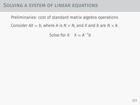
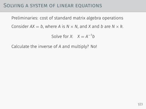
Preliminaries: cost of standard matrix algebra operations
Consider AX = b, where A is N× N, and X and b are N× k.
Solve for X: X = A−1b
Calculate the inverse of A and multiply? No!
• Directly solving for X is faster, and more stable numerically• A−1 need not even exist
> solve(A,b) # Directly solve for b> solve(A) %*% b # Return inverse and multiply
http://www.johndcook.com/blog/2010/01/19/dont-invert-that-matrix/
1/23
Solving a system of linear equations
Preliminaries: cost of standard matrix algebra operations
Consider AX = b, where A is N× N, and X and b are N× k.
Solve for X: X = A−1b
Calculate the inverse of A and multiply? No!
• Directly solving for X is faster, and more stable numerically• A−1 need not even exist
> solve(A,b) # Directly solve for b> solve(A) %*% b # Return inverse and multiply
http://www.johndcook.com/blog/2010/01/19/dont-invert-that-matrix/
1/23

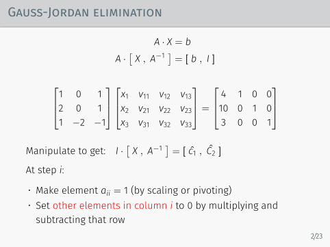
Gauss-Jordan elimination
A · X = bA ·
[X , A−1
]= [ b , I ]
1 0 12 0 11 −2 −1
x1 v11 v12 v13x2 v21 v22 v23x3 v31 v32 v33
=
4 1 0 010 0 1 03 0 0 1
Manipulate to get: I ·
[X , A−1
]= [ c1 , C2 ]
At step i:
• Make element aii = 1 (by scaling or pivoting)• Set other elements in column i to 0 by multiplying andsubtracting that row
2/23

Gauss-Jordan elimination
A · X = bA ·
[X , A−1
]= [ b , I ]
1 0 12 0 11 −2 −1
x1 v11 v12 v13x2 v21 v22 v23x3 v31 v32 v33
=
4 1 0 010 0 1 03 0 0 1
Manipulate to get: I ·[X , A−1
]= [ c1 , C2 ]
At step i:
• Make element aii = 1 (by scaling or pivoting)• Set other elements in column i to 0 by multiplying andsubtracting that row
2/23

Gauss-Jordan elimination
A · X = bA ·
[X , A−1
]= [ b , I ]
1 0 12 0 11 −2 −1
x1 v11 v12 v13x2 v21 v22 v23x3 v31 v32 v33
=
4 1 0 010 0 1 03 0 0 1
Manipulate to get: I ·
[X , A−1
]= [ c1 , C2 ]
At step i:
• Make element aii = 1 (by scaling or pivoting)• Set other elements in column i to 0 by multiplying andsubtracting that row
2/23
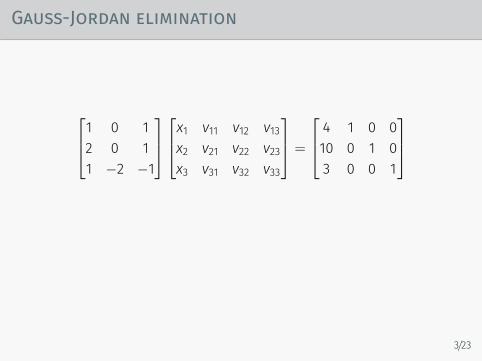
Gauss-Jordan elimination
1 0 12 0 11 −2 −1
x1 v11 v12 v13x2 v21 v22 v23x3 v31 v32 v33
=
4 1 0 010 0 1 03 0 0 1
3/23

Gauss-Jordan elimination
1 0 12 0 11 −2 −1
x1 v11 v12 v13x2 v21 v22 v23x3 v31 v32 v33
=
4 1 0 010 0 1 03 0 0 1
Multiply row 1 by 2 and subtract
3/23

Gauss-Jordan elimination
1 0 10 0 −11 −2 −1
x1 v11 v12 v13x2 v21 v22 v23x3 v31 v32 v33
=
4 1 0 02 −2 1 03 0 0 1
3/23

Gauss-Jordan elimination
1 0 10 0 −10 −2 −2
x1 v11 v12 v13x2 v21 v22 v23x3 v31 v32 v33
=
4 1 0 02 −2 1 0−1 −1 0 1
Subtract row 1
3/23

Gauss-Jordan elimination
1 0 10 −2 −20 0 −1
x1 v11 v12 v13x2 v21 v22 v23x3 v31 v32 v33
=
4 1 0 0−1 −1 0 12 −2 1 0
Pivot
3/23
Gauss-Jordan elimination
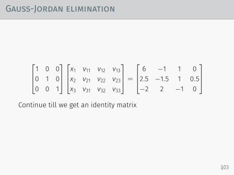
1 0 00 1 00 0 1
x1 v11 v12 v13x2 v21 v22 v23x3 v31 v32 v33
=
6 −1 1 02.5 −1.5 1 0.5−2 2 −1 0
Continue till we get an identity matrix
3/23

Gauss-Jordan elimination
1 0 00 1 00 0 1
x1 v11 v12 v13x2 v21 v22 v23x3 v31 v32 v33
=
6 −1 1 02.5 −1.5 1 0.5−2 2 −1 0
What is the cost of this algorithm?
3/23

Gauss elimination with back-substitution
A ·[X , A−1
]= [ b , I ]
O(N3) manipulation to get:
U ·[X , A−1
]= [ c1 , C2 ]
Here, U is an upper-triangular matrix.
Cannot just read off solution. Need to backsolve.
4/23

Gauss elimination with back-substitution
A ·[X , A−1
]= [ b , I ]
O(N3) manipulation to get:
U ·[X , A−1
]= [ c1 , C2 ]
Here, U is an upper-triangular matrix.
Cannot just read off solution. Need to backsolve.
4/23

Gauss elimination with back-substitution
A ·[X , A−1
]= [ b , I ]
O(N3) manipulation to get:
U ·[X , A−1
]= [ c1 , C2 ]
Here, U is an upper-triangular matrix.
Cannot just read off solution. Need to backsolve.
4/23
LU decomposition
What are we actually doing?
A = LU
Here L and U are lower and upper triangular matrices.
L =
1 0 0l21 1 0l31 l32 1
,U =
u11 u12 u130 u22 u230 0 u33
Is this always possible?
A =
[0 11 0
]
PA = LU, P is a permutation matrix
Crout’s algorithm, O(N3), stable, L,U can be computed in place.
5/23

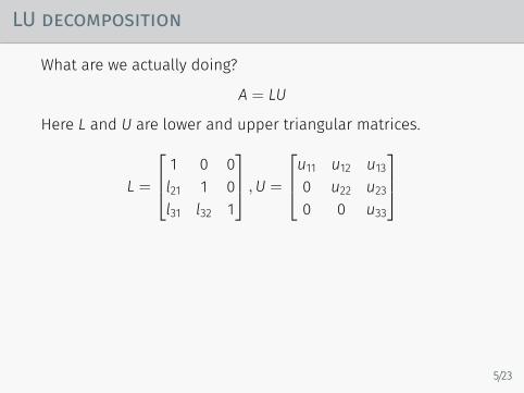
LU decomposition
What are we actually doing?
A = LU
Here L and U are lower and upper triangular matrices.
L =
1 0 0l21 1 0l31 l32 1
,U =
u11 u12 u130 u22 u230 0 u33
Is this always possible?
A =
[0 11 0
]
PA = LU, P is a permutation matrix
Crout’s algorithm, O(N3), stable, L,U can be computed in place.5/23

Backsubstitution
AX = b
LUX = Pb
First solve Y by forward substitution
LY = Pb
1 0 0l21 1 0l31 l32 1
y1y2y3
=
b1b2b3
Then solve X by back substitution
UX = Y
6/23

Backsubstitution
AX = b
LUX = Pb
First solve Y by forward substitution
LY = Pb
1 0 0l21 1 0l31 l32 1
y1y2y3
=
b1b2b3
Then solve X by back substitution
UX = Y
6/23

Backsubstitution
AX = b
LUX = Pb
First solve Y by forward substitution
LY = Pb
1 0 0l21 1 0l31 l32 1
y1y2y3
=
b1b2b3
Then solve X by back substitution
UX = Y
6/23

Backsubstitution
AX = b
LUX = Pb
First solve Y by forward substitution
LY = Pb
1 0 0l21 1 0l31 l32 1
y1y2y3
=
b1b2b3
Then solve X by back substitution
UX = Y6/23

Comments
• LU-decomposition can be reused for different b’s.• Calculating LU decomposition: O(N3).• Given LU decomposition, solving for X: O(N2).• |A| = |P−1LU| = (−1)S
∏Ni=1 uii (S: num. of exchanges)
• LUA−1 = PI, can solve for A−1. (back to Gauss-Jordan)
7/23

Cholesky decomposition
If A is symmetric positive-definite:
A = LLT (but now L need not have a diagonal of ones)
• ‘Square-root’ of A• More stable.• Twice as efficient.• Related: A = LDLT (but now L has a unit diagonal).
8/23

Eigenvalue decomposition
An N× N matrix A: a map from RN → RN.An eigenvector v undergoes no rotation:
Av = λv
λ is the corresponding eigenvalue, and gives the ‘rescaling’.
Let Λ = diag(λ1, · · · , λN) with λ1 ≥ λ2, . . . , λN, andV = [v1, · · · , vN] be the matrix of corresponding eigenvectors
AV = VΛ
Real Symmetric matrices have
• real eigenvalues• different eigenvalues have orthogonal eigenvectors
9/23
Calculating eigenvalues and -vectors
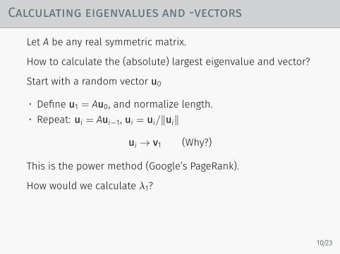
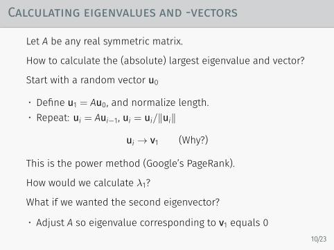
Let A be any real symmetric matrix.
How to calculate the (absolute) largest eigenvalue and vector?
Start with a random vector u0
• Define u1 = Au0, and normalize length.• Repeat: ui = Aui−1, ui = ui/∥ui∥
ui → v1 (Why?)
This is the power method (Google’s PageRank).
How would we calculate λ1?
What if we wanted the second eigenvector?
• Adjust A so eigenvalue corresponding to v1 equals 0
10/23

Calculating eigenvalues and -vectors
Let A be any real symmetric matrix.
How to calculate the (absolute) largest eigenvalue and vector?
Start with a random vector u0
• Define u1 = Au0, and normalize length.• Repeat: ui = Aui−1, ui = ui/∥ui∥
ui → v1 (Why?)
This is the power method (Google’s PageRank).
How would we calculate λ1?
What if we wanted the second eigenvector?
• Adjust A so eigenvalue corresponding to v1 equals 0
10/23
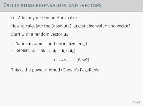
Calculating eigenvalues and -vectors
Let A be any real symmetric matrix.
How to calculate the (absolute) largest eigenvalue and vector?
Start with a random vector u0
• Define u1 = Au0, and normalize length.• Repeat: ui = Aui−1, ui = ui/∥ui∥
ui → v1 (Why?)
This is the power method (Google’s PageRank).
How would we calculate λ1?
What if we wanted the second eigenvector?
• Adjust A so eigenvalue corresponding to v1 equals 0
10/23
Calculating eigenvalues and -vectors
Let A be any real symmetric matrix.
How to calculate the (absolute) largest eigenvalue and vector?
Start with a random vector u0
• Define u1 = Au0, and normalize length.• Repeat: ui = Aui−1, ui = ui/∥ui∥
ui → v1 (Why?)
This is the power method (Google’s PageRank).
How would we calculate λ1?
What if we wanted the second eigenvector?
• Adjust A so eigenvalue corresponding to v1 equals 010/23

Gauss-Jordan elimination10 7 8 77 5 6 58 6 10 97 5 9 10
x1x2x3x4
=
32233331
What is the solution? How about for b = [32.1, 22.9, 33.1, 30.9]T?
Why the difference?
• the determinant?• the inverse?• the condition number?
An ill-conditioned problem can strongly amplify errors.
• Even without any rounding error
11/23

Stability analysis
The operator norm of a matrix A is
∥A∥2 = ∥A∥ = max∥v∥=1
∥Av∥ = maxv
∥Av∥∥v∥
For a symmetric, real matrix, ∥A∥ = λmax(A) (why?)
For a general, real matrix, ∥A∥ =√
λmax(ATA) (why?)
For A in RN×N and any v ∈ RN,
∥Av∥ ≤ ∥A∥∥v∥ (why?)
If A = BC, and all matrices are in RN×N,
∥A∥ ≤ ∥B∥∥C∥ (why?)
12/23
Stability analysis
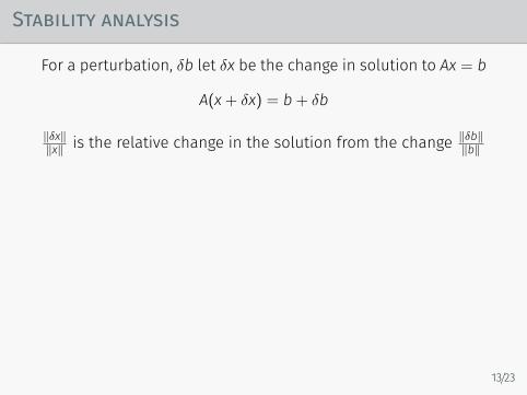
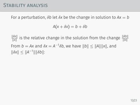
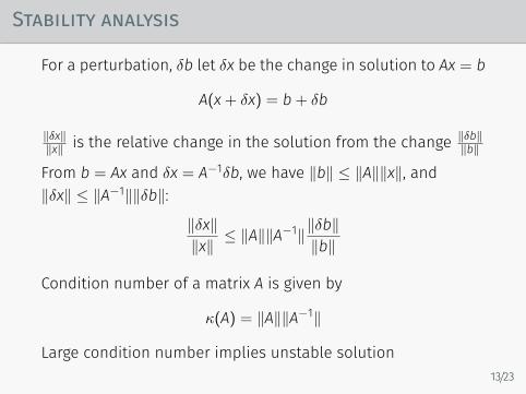
For a perturbation, δb let δx be the change in solution to Ax = b
A(x+ δx) = b+ δb
∥δx∥∥x∥ is the relative change in the solution from the change ∥δb∥
∥b∥
From b = Ax and δx = A−1δb, we have ∥b∥ ≤ ∥A∥∥x∥, and∥δx∥ ≤ ∥A−1∥∥δb∥:
∥δx∥∥x∥ ≤ ∥A∥∥A−1∥∥δb∥
∥b∥
Condition number of a matrix A is given by
κ(A) = ∥A∥∥A−1∥
Large condition number implies unstable solution
13/23
Stability analysis
For a perturbation, δb let δx be the change in solution to Ax = b
A(x+ δx) = b+ δb
∥δx∥∥x∥ is the relative change in the solution from the change ∥δb∥
∥b∥
From b = Ax and δx = A−1δb, we have ∥b∥ ≤ ∥A∥∥x∥, and∥δx∥ ≤ ∥A−1∥∥δb∥:
∥δx∥∥x∥ ≤ ∥A∥∥A−1∥∥δb∥
∥b∥
Condition number of a matrix A is given by
κ(A) = ∥A∥∥A−1∥
Large condition number implies unstable solution
13/23
Stability analysis
For a perturbation, δb let δx be the change in solution to Ax = b
A(x+ δx) = b+ δb
∥δx∥∥x∥ is the relative change in the solution from the change ∥δb∥
∥b∥
From b = Ax and δx = A−1δb, we have ∥b∥ ≤ ∥A∥∥x∥, and∥δx∥ ≤ ∥A−1∥∥δb∥:
∥δx∥∥x∥ ≤ ∥A∥∥A−1∥∥δb∥
∥b∥
Condition number of a matrix A is given by
κ(A) = ∥A∥∥A−1∥
Large condition number implies unstable solution13/23
Stability analysis
κ(A) ≥ 1 (why?)
For a real symmetric matrix, κ(A) = λmax(A)λmin(A)
(why?)
For a real matrix, κ(A) =√
λmax(ATA)λmin(ATA)
(why?)
Condition number is a property of a problem
Stability is a property of an algorithm
A bad algorithm can mess up a simple problem
14/23
Stability analysis
κ(A) ≥ 1 (why?)
For a real symmetric matrix, κ(A) = λmax(A)λmin(A)
(why?)
For a real matrix, κ(A) =√
λmax(ATA)λmin(ATA)
(why?)
Condition number is a property of a problem
Stability is a property of an algorithm
A bad algorithm can mess up a simple problem
14/23
Stability analysis
κ(A) ≥ 1 (why?)
For a real symmetric matrix, κ(A) = λmax(A)λmin(A)
(why?)
For a real matrix, κ(A) =√
λmax(ATA)λmin(ATA)
(why?)
Condition number is a property of a problem
Stability is a property of an algorithm
A bad algorithm can mess up a simple problem
14/23

Stability analysis
κ(A) ≥ 1 (why?)
For a real symmetric matrix, κ(A) = λmax(A)λmin(A)
(why?)
For a real matrix, κ(A) =√
λmax(ATA)λmin(ATA)
(why?)
Condition number is a property of a problem
Stability is a property of an algorithm
A bad algorithm can mess up a simple problem
14/23
Gaussian elimination with partial pivoting
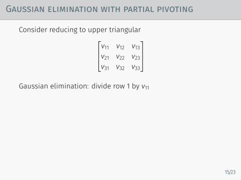
Consider reducing to upper triangularv11 v12 v13v21 v22 v23v31 v32 v33
Gaussian elimination: divide row 1 by v11
[1e− 4 11 1
]
Partial pivoting: Pivot rows to bring maxr vr1 to top
Can dramatically improve performance. E.g.
Why does it work?
15/23

Gaussian elimination with partial pivoting
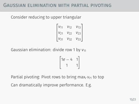
Consider reducing to upper triangularv11 v12 v13v21 v22 v23v31 v32 v33
Gaussian elimination: divide row 1 by v11[
1e− 4 11 1
]
Partial pivoting: Pivot rows to bring maxr vr1 to top
Can dramatically improve performance. E.g.
Why does it work?
15/23
Gaussian elimination with partial pivoting
Consider reducing to upper triangularv11 v12 v13v21 v22 v23v31 v32 v33
Gaussian elimination: divide row 1 by v11[
1e− 4 11 1
]
Partial pivoting: Pivot rows to bring maxr vr1 to top
Can dramatically improve performance. E.g.
Why does it work?
15/23

Gaussian elimination with partial pivoting
Consider reducing to upper triangularv11 v12 v13v21 v22 v23v31 v32 v33
Gaussian elimination: divide row 1 by v11[
1e− 4 11 1
]
Partial pivoting: Pivot rows to bring maxr vr1 to top
Can dramatically improve performance. E.g.
Why does it work?15/23

Gaussian elimination with partial pivoting
Recall Gaussian elimination decomposes A = LU and solvestwo intermediate problems.
What are the condition numbers of L and U?
Try[1e− 4 11 1
]Note: R does pivoting for you automatically! (see the functionlu in package Matrix)
16/23

QR decomposition
In general, for A = BC, κ(A) ≤ κ(B)κ(C) (why?)
QR decomposition:A = QR
Here, R is an upper (right) triangular matrix. Q is anorthonormal matrix: QTQ = I
κ(A) = κ(Q)κ(R) (why?)
Can use to solve Ax = b (How?)
Most stable decomposition
Does this mean we should use QR decomposition?
17/23

Gram-Schmidt orthonormalization
Given N vectors x1, . . . , xN construct an orthonormal basis:
u1 = x1/∥x1∥
ui = xi −∑i−1
j=1(xTi uj)ui, ui = ui/∥ui∥ i = 2 . . . ,N
18/23

Gram-Schmidt orthonormalization
Given N vectors x1, . . . , xN construct an orthonormal basis:
u1 = x1/∥x1∥
ui = xi −∑i−1
j=1(xTi uj)ui, ui = ui/∥ui∥ i = 2 . . . ,N
18/23

QR decomposition
A = Q R
a11 a12 a13a21 a22 a23a31 a32 a33
=
q11 q12 q13q21 q22 q23q31 q32 q33
r11 r12 r130 r22 r230 0 r33
QR decomposition: Gram-Schmidt on columns of A(can you see why?)
Of course, there are more stable/efficient ways of doing this(Householder rotation/Givens rotation)
O(N3) algorithms (though about twice as slow as LU)
19/23

QR decomposition
A = Q R
a11 a12 a13a21 a22 a23a31 a32 a33
=
q11 q12 q13q21 q22 q23q31 q32 q33
r11 r12 r130 r22 r230 0 r33
QR decomposition: Gram-Schmidt on columns of A(can you see why?)
Of course, there are more stable/efficient ways of doing this(Householder rotation/Givens rotation)
O(N3) algorithms (though about twice as slow as LU)19/23

QR algorithm
Algorithm to calculate all eigenvalues/eigenvectors of a (nottoo-large) matrix
Start with A0 = A. At iteration i:
• Ai = QiRi• Ai+1 = RiQi
Then Ai and Ai+1 have the same eigenvalues (why?), and thediagonal contains the eigenvalues.
Can be made morestable/efficient.
One of Dongarra & Sullivan (2000)’s list of top 10 algoirithms.https://www.siam.org/pdf/news/637.pdf
See also number 4, ”decompositional approach to matrixcomputations”
20/23

QR algorithm
Algorithm to calculate all eigenvalues/eigenvectors of a (nottoo-large) matrix
Start with A0 = A. At iteration i:
• Ai = QiRi• Ai+1 = RiQi
Then Ai and Ai+1 have the same eigenvalues (why?), and thediagonal contains the eigenvalues. Can be made morestable/efficient.
One of Dongarra & Sullivan (2000)’s list of top 10 algoirithms.https://www.siam.org/pdf/news/637.pdf
See also number 4, ”decompositional approach to matrixcomputations”
20/23

Multivariate normal
log(p(X|µ,Σ)) = − 12(X− µ)TΣ−1(X− µ)− N2 log 2π − 1
2 log |Σ|
Σ = LLT
Y = L−1(X− µ) (Forward solve)
log(p(X|µ,Σ)) = − 12YTY− N
2 log 2π − log |Σ|
Can also just forward solve for L−1: LL−1 = I(Inverted triangular matrix isn’t too bad)
21/23

Multivariate normal
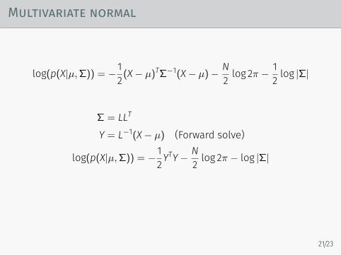
log(p(X|µ,Σ)) = − 12(X− µ)TΣ−1(X− µ)− N2 log 2π − 1
2 log |Σ|
Σ = LLT
Y = L−1(X− µ) (Forward solve)
log(p(X|µ,Σ)) = − 12YTY− N
2 log 2π − log |Σ|
Can also just forward solve for L−1: LL−1 = I(Inverted triangular matrix isn’t too bad)
21/23
Multivariate normal
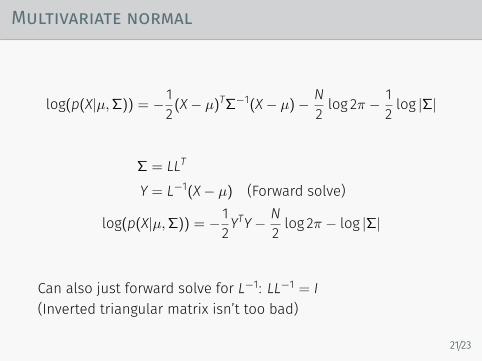
log(p(X|µ,Σ)) = − 12(X− µ)TΣ−1(X− µ)− N2 log 2π − 1
2 log |Σ|
Σ = LLT
Y = L−1(X− µ) (Forward solve)
log(p(X|µ,Σ)) = − 12YTY− N
2 log 2π − log |Σ|
Can also just forward solve for L−1: LL−1 = I(Inverted triangular matrix isn’t too bad)
21/23
Multivariate normal
log(p(X|µ,Σ)) = − 12(X− µ)TΣ−1(X− µ)− N2 log 2π − 1
2 log |Σ|
Σ = LLT
Y = L−1(X− µ) (Forward solve)
log(p(X|µ,Σ)) = − 12YTY− N
2 log 2π − log |Σ|
Can also just forward solve for L−1: LL−1 = I(Inverted triangular matrix isn’t too bad)
21/23

Sampling a multivariate normal
Sampling a univariate normal:
• Inversion method (default for rnorm?).• Box-Muller transform: (Z1, Z2) : independent standardnormals.
• Let Z ∼ N (0, I)• X = µ+ LZ• Z = N (µ, LTL)
22/23

Sampling a multivariate normal
Sampling a univariate normal:
• Inversion method (default for rnorm?).• Box-Muller transform: (Z1, Z2) : independent standardnormals.
• Let Z ∼ N (0, I)• X = µ+ LZ• Z = N (µ, LTL)
22/23

−10
−5
0
5
10
−10 −5 0 5 10y
x
Σ =
[1 00 1
]
23/23

−10
−5
0
5
10
−10 −5 0 5 10y
x
Σ =
[4 00 1
]
23/23

−10
−5
0
5
10
−10 −5 0 5 10y
x
Σ =
[4 22 4
]
23/23

−10
−5
0
5
10
−10 −5 0 5 10y
x
Σ =
[4 3.83.8 4
]
23/23