Embed Size (px)
Citation preview

3.012 Fundamentals of Materials Science Fall 2005
Lecture 17: 11.07.05 Free Energy of Multi-phase Solutions at Equilibrium
Today:
LAST TIME .........................................................................................................................................................................................2FREE ENERGY DIAGRAMS OF MULTI-PHASE SOLUTIONS1 ................................................................................................................3
The common tangent construction and the lever rule ...............................................................................................................3Practical sources of free energy data .........................................................................................................................................8
INTRODUCTION TO BINARY PHASE DIAGRAMS.................................................................................................................................9Phase diagram of an ideal solution ............................................................................................................................................9Tie lines and the lever rule on a binary phase diagram..........................................................................................................10
BINARY SOLUTIONS WITH LIMITED MISCIBILITY: MISCIBILITY GAPS...........................................................................................11The Regular Solution Model, part I ..........................................................................................................................................11
REFERENCES ...................................................................................................................................................................................14
: Lupis, Chemical Thermodynamics of Materials, Ch 8 ‘Binary Phase Diagrams,’Readingpp. 196-203
Supplementary Reading: -
Lecture 18 – Multi-phase Equilibria 1 of 14 11/6/05
3.012 Fundamentals of Materials Science Fall 2005
Last time
Lecture 18 – Multi-phase Equilibria 2 of 14 11/6/05

3.012 Fundamentals of Materials Science Fall 2005
Free energy diagrams of multi-phase solutions1
• Last lecture we examined the structure and interpretation of free energy vs. composition diagrams for ideal binary (two-component) solutions. The free energy diagrams we introduced last time can conveniently be also used to analyze multiphase equilibria that allow us to graphically depict the requirements for equilibrium.
The common tangent construction and the lever rule
• KEY CONCEPTS: Free energy vs. composition diagrams are useful tools for graphically analyzing phase equilibria in binary systems at constant pressure. Common tangents between the free energy curves of different phases occur in regions where 2 phases are in equilibrium. The points where common tangents touch the free energy curves identify the compositions of the two phases in equilibrium. The lever rule is used to determine how much of each phase is present in two phase equilibrium regions.
• Suppose we have a binary ideal solution of A and B. We showed last time the shape of the free energy curve for such a solution. The molar free energy for the solution can be diagrammed for different phases of the solution- for example the liquid state and the solid state- as a function of composition:
o Suppose we lowered the temperature from the above situation. How would the two free energy curves change? Which curve will move more, considering that:
!
G = H "TS
Lecture 18 – Multi-phase Equilibria 3 of 14 11/6/05

3.012 Fundamentals of Materials Science Fall 2005
o What is happening in the second figure? We have reduced the temperature to the point where the stable state of pure B is a solid. Remember that the chemical potential is given by the end-
Lecture 18 – Multi-phase Equilibria 4 of 14 11/6/05
3.012 Fundamentals of Materials Science Fall 2005
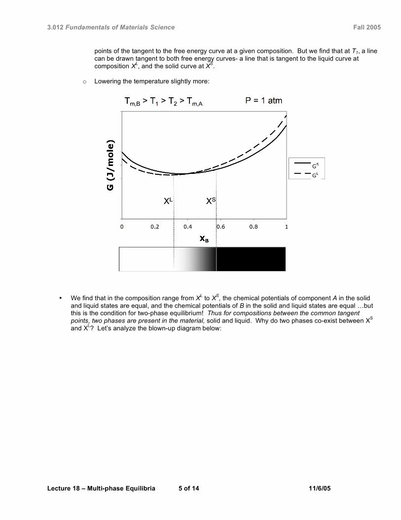
points of the tangent to the free energy curve at a given composition. But we find that at T1, a line can be drawn tangent to both free energy curves- a line that is tangent to the liquid curve at composition XL, and the solid curve at XS .
o Lowering the temperature slightly more:
• We find that in the composition range from XL to XS, the chemical potentials of component A in the solid and liquid states are equal, and the chemical potentials of B in the solid and liquid states are equal …but this is the condition for two-phase equilibrium! Thus for compositions between the common tangent points, two phases are present in the material, solid and liquid. Why do two phases co-exist between XS
and XL? Let’s analyze the blown-up diagram below:
Lecture 18 – Multi-phase Equilibria 5 of 14 11/6/05

3.012 Fundamentals of Materials Science Fall 2005
• At composition X1, comparison of the solid state free energy with that of the liquid shows that the liquid would be the form with lowest free energy- thus the liquid solution would be more stable than the solid. However, the free energy of the liquid is not the lowest possible free energy state. If the A and B atoms in the homogenous liquid solution re-arrange, a portion transforming to a solid with composition XS and a portion remaining in a li
!
G sep
quid solution with composition altered to XL, the heterogeneous solid/liquid mixture takes on the free energy , which is lower than that of the homogeneous liquid solution at X1 . f L and f S are the phase fractions of liquid and solid phases, respectively. Note that because a heterogeneous (2-phase) mixture is being formed, the free energy is determined in a manner similar to that discussed earlier for heterogeneous mixtures (e.g. our block of Si in contact with a block of Ge)- simply a weighted average of the molar free energies of the liquid phase (composition XL) and the solid phase (composition XS).
Lecture 18 – Multi-phase Equilibria 6 of 14 11/6/05
3.012 Fundamentals of Materials Science Fall 2005
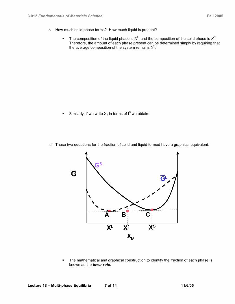
o How much solid phase forms? How much liquid is present?
The composition of the liquid phase is XL, and the composition of the solid phase is XS . Therefore, the amount of each phase present can be determined simply by requiring that the average composition of the system remains X1:
Similarly, if we write X1 in terms of fS we obtain:
o These two equations for the fraction of solid and liquid formed have a graphical equivalent:
The mathematical and graphical construction to identify the fraction of each phase is known as the lever rule.
Lecture 18 – Multi-phase Equilibria 7 of 14 11/6/05

3.012 Fundamentals of Materials Science Fall 2005
Practical sources of free energy data
• Where do we get the information for these diagrams?
o National Institute of Standards and Technology Chemistry WebBook http://webbook.nist.gov/chemistry heat capacity, enthalpy, and entropy data
o JANAF Tables Joint Army Navy Air Force database of thermochemical data Exhaustive Cp, entropy, enthalpy, free energy data QD511.J74. 1986
o Selected Values of Thermodynamic Properties of Metals and Alloys R. Hultgren, R.L. Orr, P.D. Anderson, and K.K. Kelley John Wiley, NY 1963 QD171.S44
o Thermo-Calc Software available on Athena for performing many thermodynamic calculations, building
phase diagrams, etc.
Lecture 18 – Multi-phase Equilibria 8 of 14 11/6/05

3.012 Fundamentals of Materials Science Fall 2005
Introduction to binary phase diagrams
• KEY CONCEPTS: The phase equilibria as a function of composition for a fixed temperature (and fixed pressure) predicted by Free energy vs. composition diagrams can be collated to create a binary phase diagram, which maps out stable phases in T vs. composition space (pressure assume fixed)—the binary system analog of single component phase diagrams. The Gibbs phase rule can be applied to these diagrams, accounting for the fixed pressure (D + P = C + 1). Tie lines allow the lever rule to be directly applied to phase diagrams in order to calculate the amount of each phase present in multiphase equilibria.
Phase diagram of an ideal solution
• From an examination of free energy vs. composition diagrams, we found that phase separation (induced for example by reducing the temperature and freezing a liquid solution) proceeds by the following progression across the composition window of an ideal binary solution (For a system where Tm,B > Tm,A):
T > Tm,B > Tm,A
Tm,B > T1 > Tm,A
Tm,B > T1 > T2 > Tm,A
T = Tm,B > Tm,A
Tm,B > T = Tm,A
Tm,B > T2 > T3 > Tm,A
• It would make sense to obtain a continuous map of the phases present as a function of XB and temperature for a binary system: such a map is a key tool in materials science & engineering and is known as a binary phase diagram. For the ideal binary solution we have been analyzing, the phase diagram looks like this:
Lecture 18 – Multi-phase Equilibria 9 of 14 11/6/05

3.012 Fundamentals of Materials Science Fall 2005
two-phase
region
T
Homogeneous liquid mixture
Homogeneous solid mixture
Tm
Tm (pure B)
1
2
KB
P = constant
(pure A)
T = T
T = T
Figure by MIT OCW.
• This is the simplest form a binary phase diagram can take.
Tie lines and the lever rule on a binary phase diagram
• The lever rule that we developed using free energy vs. composition diagrams can be directly applied to a binary phase diagram (T vs. composition). This is done using tie lines—horizontal isotherms connecting the boundaries of a two-phase region:
Lecture 18 – Multi-phase Equilibria 10 of 14 11/6/05
3.012 Fundamentals of Materials Science Fall 2005
Binary solutions with limited miscibility: Miscibility gaps
The Regular Solution Model, part I
• What happens if the molecules in the so
!
"H mix
< 0
lution interact with a finite energy? The en
!
"H mix
> 0
thalpy of mixing will now have a finite value, either favoring ( ) or disfavoring ( ) mixing of the two components. The simplest model of a solution with finite interactions is called the regular solution model:
o Let the enthalpy of mixing take on a finite value given by:
o We take the entropy of mixing to be the same as in the ideal solution. This gives a total free energy of mixing which is:
o The regular solution model describes the liquid phase of many real systems such as Pb-Sn, Ga-Sb, and Tl-Sn, and some solid solutions. Today we will analyze the behavior of a system with this free energy function; in a few lectures we will show how the given forms of the enthalpy and entropy of mixing arise from consideration of molecular states (using statistical mechanics).
Lecture 18 – Multi-phase Equilibria 11 of 14 11/6/05

3.012 Fundamentals of Materials Science Fall 2005
-3000
-2000
-1000
0
1000
2000
3000
4000
5000
6000
0 0.2 0.4 0.6 0.8 1
XB
T=100 K
!Hmix,RS
XB
" = 20,000 J/mole
" = 10,000 J/mole
" = -10,000 J/mole
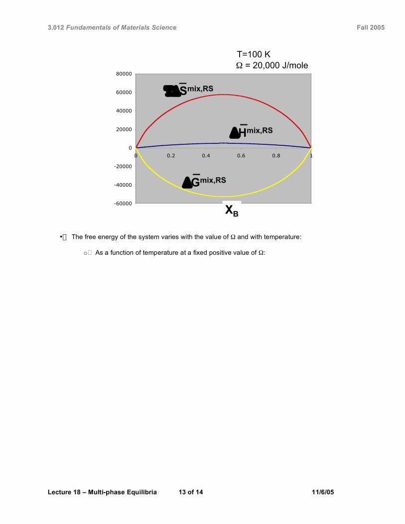
o The overall free energy of mixing arises from the balance between favorable mixing entropy and unfavorable enthalpy contributions:
Lecture 18 – Multi-phase Equilibria 12 of 14 11/6/05
3.012 Fundamentals of Materials Science Fall 2005
-60000
-40000
-20000
0
20000
40000
60000
80000
0 0.2 0.4 0.6 0.8 1
T=100 K
!Hmix,RS
XB
" = 20,000 J/mole
!Gmix,RS
#!Smix,RS
• The free energy of the system varies with the value of Ω and with temperature:
o As a function of temperature at a fixed positive value of Ω:
Lecture 18 – Multi-phase Equilibria 13 of 14 11/6/05

3.012 Fundamentals of Materials Science Fall 2005
References
1. Carter, W. C. 3.00 Thermodynamics of Materials Lecture Notes http://pruffle.mit.edu/3.00/ (2002).
Lecture 18 – Multi-phase Equilibria 14 of 14 11/6/05