Lecture 16 1

2nd Order Circuits

Lecture 16 2

2nd Order Circuits

• Any circuit with a single capacitor, a single inductor, an arbitrary number of sources, and an arbitrary number of resistors is a circuit of order 2.

• Any voltage or current in such a circuit is the solution to a 2nd order differential equation.

Lecture 16 3

Important Concepts

• The differential equation

• Forced and homogeneous solutions

• The natural frequency and the damping ratio

Lecture 16 4

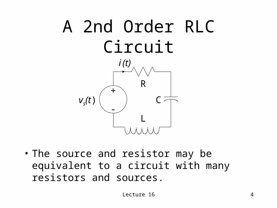
A 2nd Order RLC Circuit

• The source and resistor may be equivalent to a circuit with many resistors and sources.

R+

-Cvs(t)

i (t)

L

Lecture 16 5

Applications Modeled by a 2nd Order RLC Circuit

• Filters

– A bandpass filter such as the IF amp for the AM radio.

– A lowpass filter with a sharper cutoff than can be obtained with an RC circuit.

Lecture 16 6

The Differential Equation

KCL around the loop:

vr(t) + vc(t) + vl(t) = vs(t)

R+

-Cvs(t)

+

-

vc(t)

+ -vr(t)

L

+ -vl(t)

i (t)

Lecture 16 7

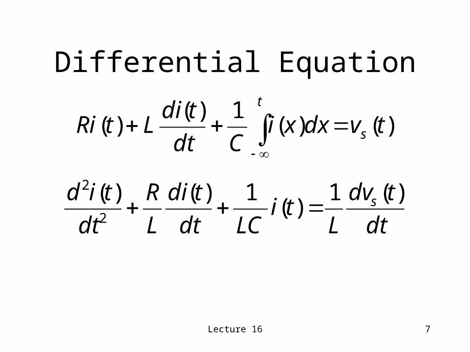
Differential Equation

)()(1)(

)( tvdxxiCdt

tdiLtRi s

t

dt

tdv

Lti

LCdt

tdi

L

R

dt

tid s )(1)(

1)()(2

2

Lecture 16 8

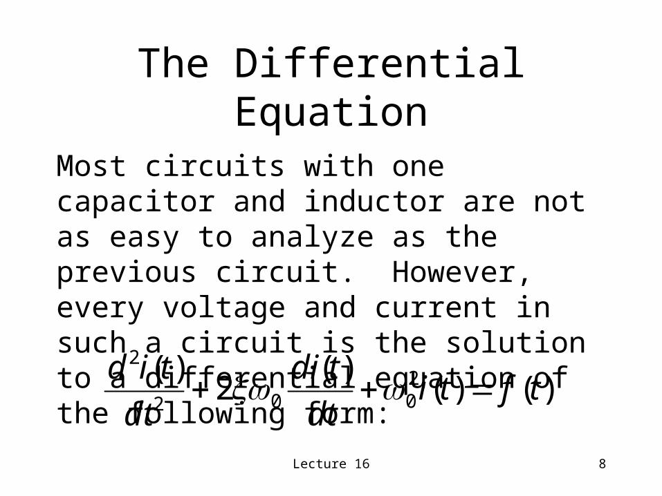
The Differential Equation

Most circuits with one capacitor and inductor are not as easy to analyze as the previous circuit. However, every voltage and current in such a circuit is the solution to a differential equation of the following form:

)()()(

2)( 2

002

2

tftidt

tdi

dt

tid

Lecture 16 9

Important Concepts

• The differential equation

• Forced and homogeneous solutions

• The natural frequency and the damping ratio

Lecture 16 10

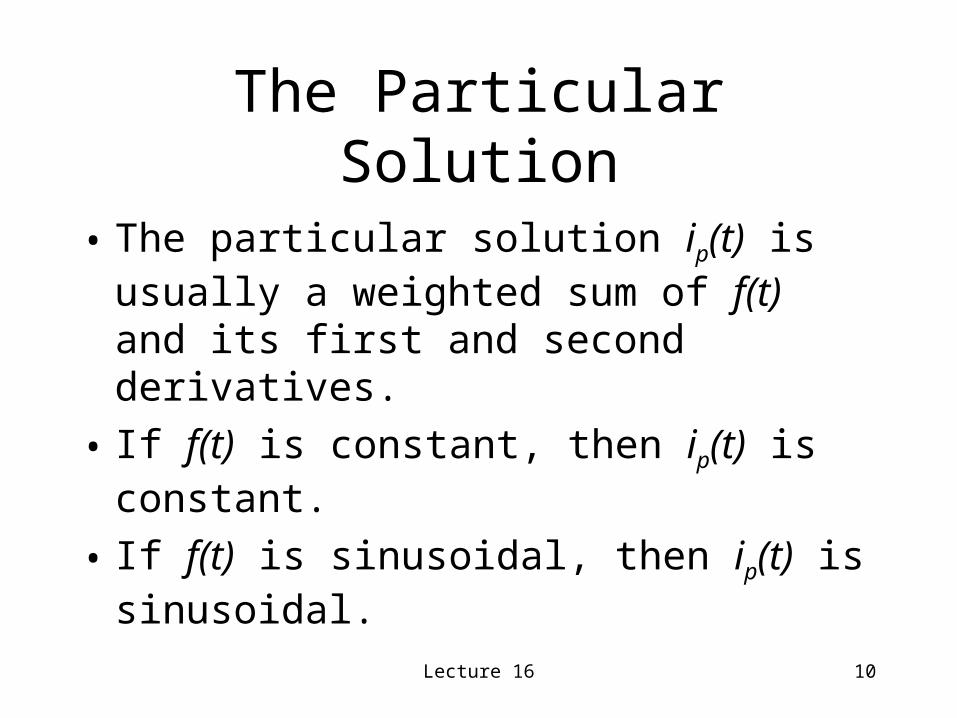
The Particular Solution

• The particular solution ip(t) is usually a weighted sum of f(t) and its first and second derivatives.

• If f(t) is constant, then ip(t) is constant.

• If f(t) is sinusoidal, then ip(t) is sinusoidal.

Lecture 16 11

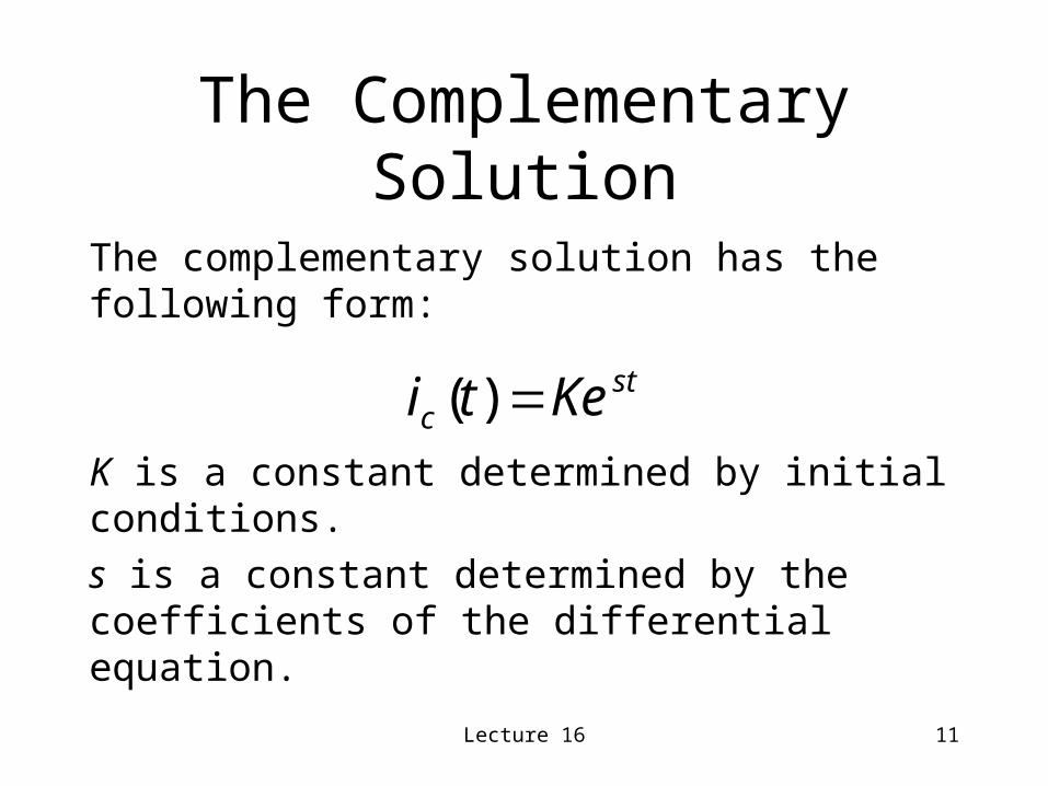
The Complementary Solution

The complementary solution has the following form:

K is a constant determined by initial conditions.

s is a constant determined by the coefficients of the differential equation.

stc Keti )(

Lecture 16 12

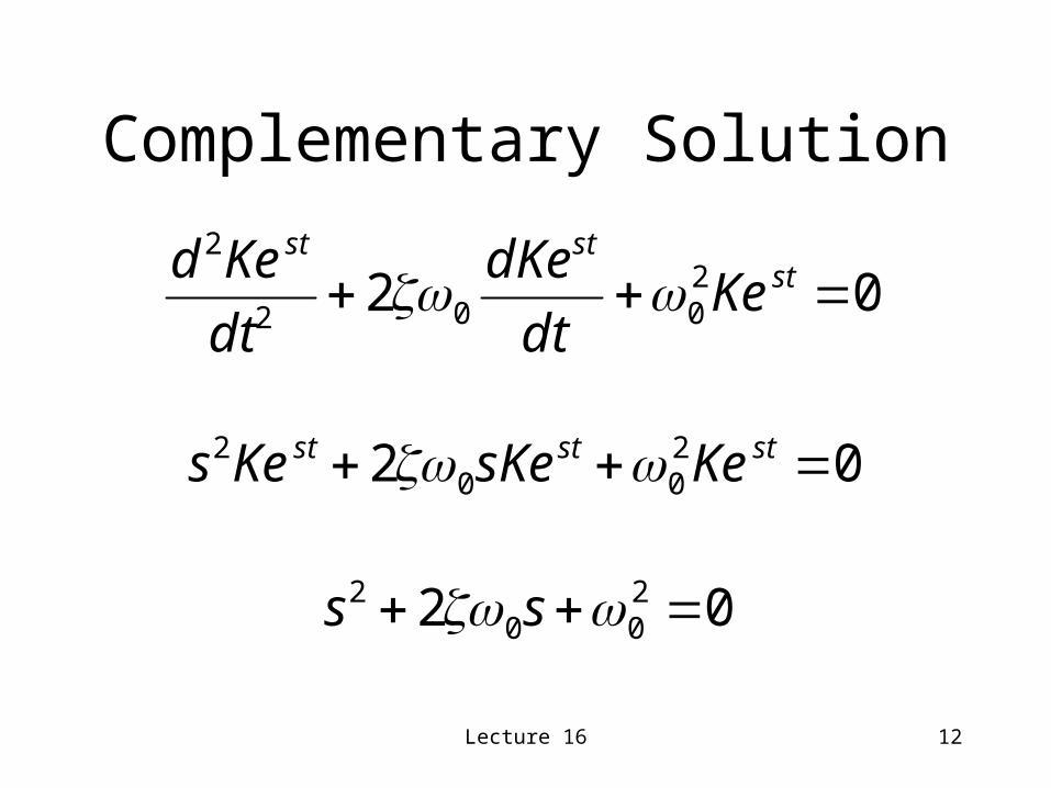
Complementary Solution

02 2002

2

ststst

Kedt

dKe

dt

Ked

02 200

2 ststst KesKeKes

02 200

2 ss

Lecture 16 13

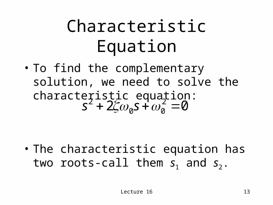
Characteristic Equation

• To find the complementary solution, we need to solve the characteristic equation:

• The characteristic equation has two roots-call them s1 and s2.

02 200

2 ss

Lecture 16 14

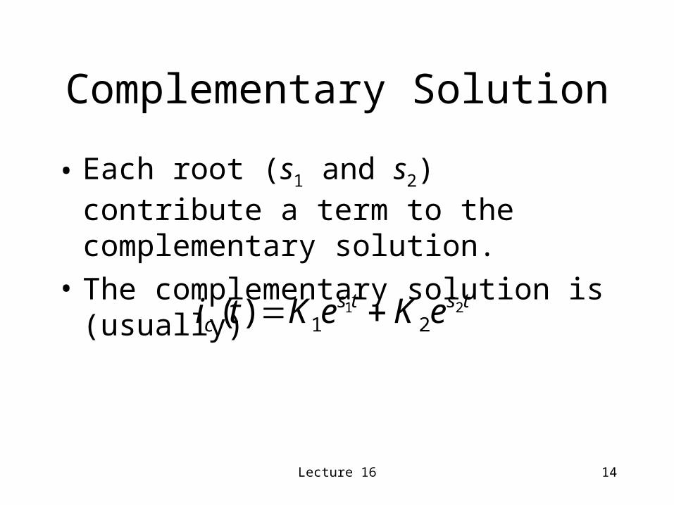
Complementary Solution

• Each root (s1 and s2) contribute a term to the complementary solution.

• The complementary solution is (usually)

tstsc eKeKti 21

21)(

Lecture 16 15

Important Concepts

• The differential equation

• Forced and homogeneous solutions

• The natural frequency and the damping ratio

Lecture 16 16

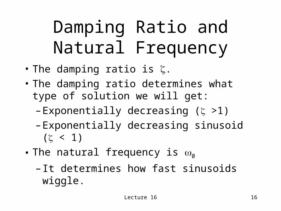
Damping Ratio and Natural Frequency

• The damping ratio is .

• The damping ratio determines what type of solution we will get:

– Exponentially decreasing ( >1)

– Exponentially decreasing sinusoid ( < 1)

• The natural frequency is 0

– It determines how fast sinusoids wiggle.

Lecture 16 17

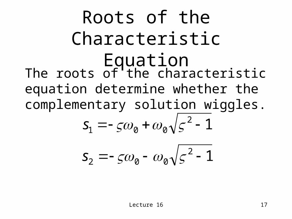
Roots of the Characteristic Equation

The roots of the characteristic equation determine whether the complementary solution wiggles.

12001 s

12002 s

Lecture 16 18

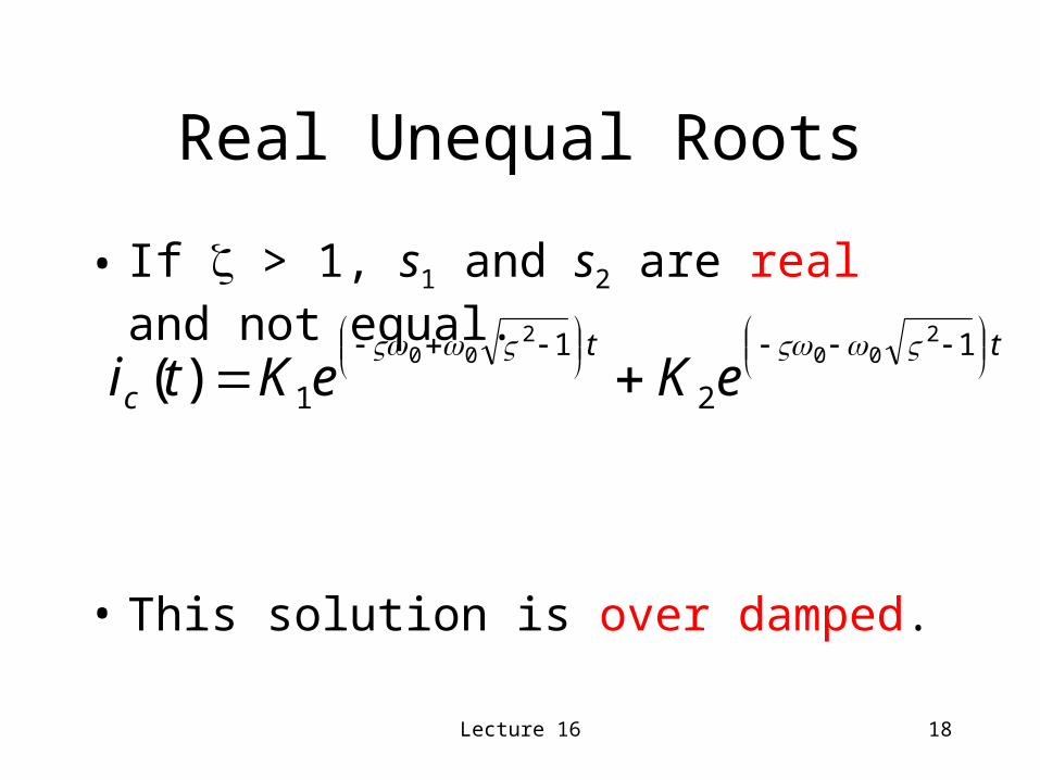
Real Unequal Roots

• If > 1, s1 and s2 are real and not equal.

• This solution is over damped.

tt

c eKeKti

1

2

1

1

200

200

)(

Lecture 16 19

Over Damped

0

0.2

0.4

0.6

0.8

1

-1.00E-06

t

i(t)

-0.2

0

0.2

0.4

0.6

0.8

-1.00E-06

ti(t)

Lecture 16 20

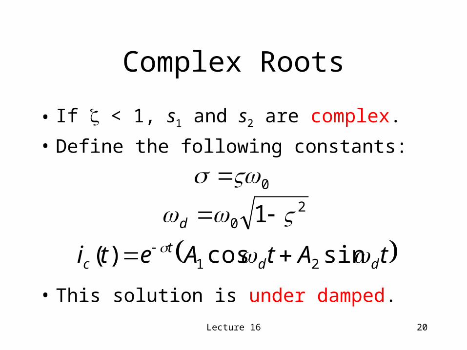
Complex Roots

• If < 1, s1 and s2 are complex.

• Define the following constants:

• This solution is under damped.

tAtAeti ddt

c sincos)( 21

0 2

0 1 d

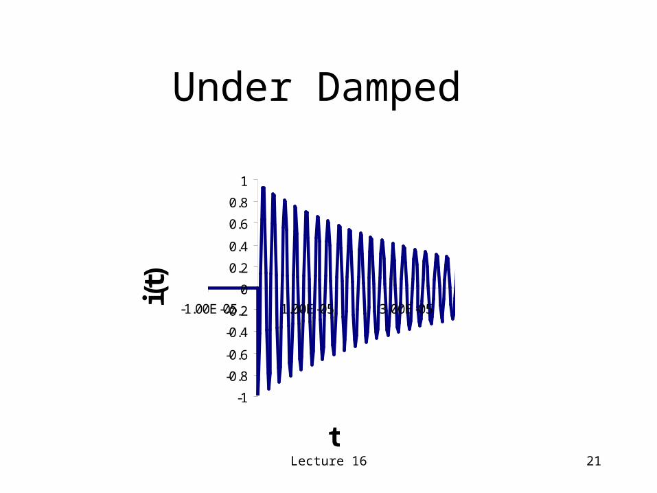
Lecture 16 21

Under Damped

-1

-0.8

-0.6

-0.4

-0.2

0

0.2

0.4

0.6

0.8

1

-1.00E-05 1.00E-05 3.00E-05

t

i(t)

Lecture 16 22

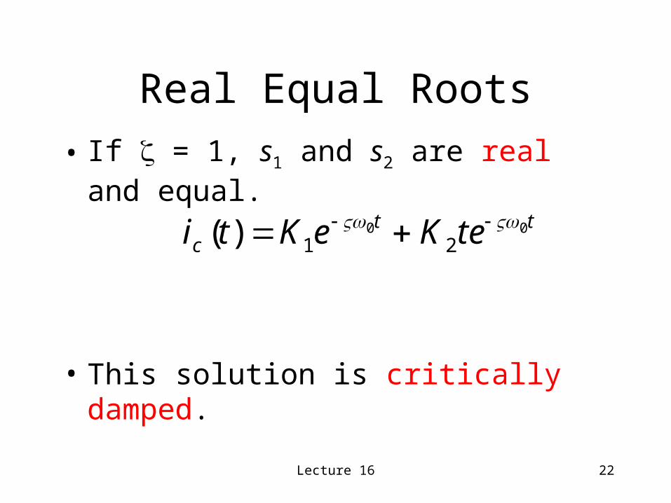
Real Equal Roots

• If = 1, s1 and s2 are real and equal.

• This solution is critically damped.

ttc teKeKti 00

21)(

Lecture 16 23

Example

• This is one possible implementation of the filter portion of the IF amplifier.

10+

-769pFvs(t)

i (t)

159H

Lecture 16 24

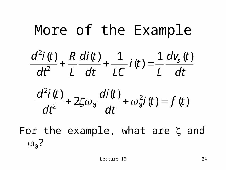
More of the Example

dt

tdv

Lti

LCdt

tdi

L

R

dt

tid s )(1)(

1)()(2

2

)()()(

2)( 2

002

2

tftidt

tdi

dt

tid

For the example, what are and 0?

Lecture 16 25

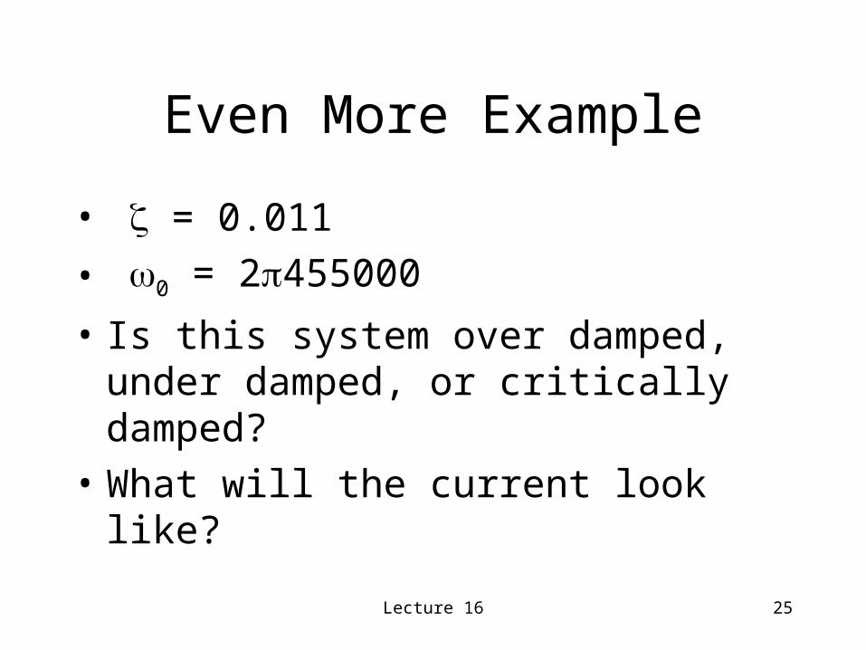
Even More Example

• = 0.011

• 0 = 2455000

• Is this system over damped, under damped, or critically damped?

• What will the current look like?

Lecture 16 26

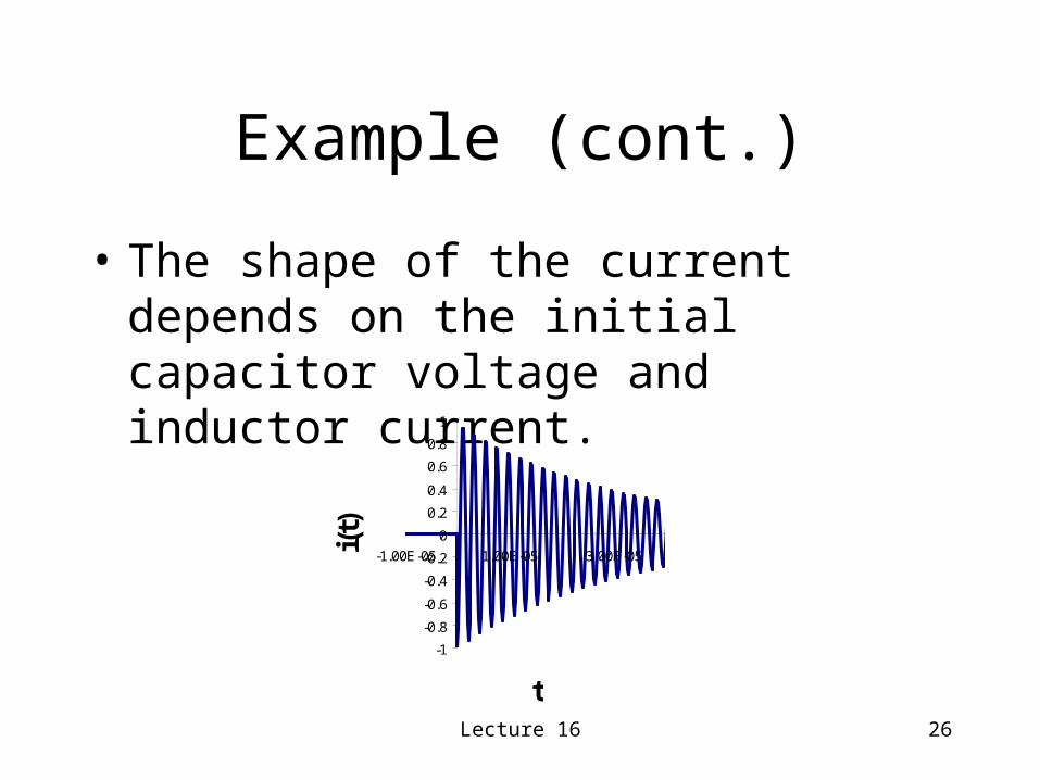
Example (cont.)

• The shape of the current depends on the initial capacitor voltage and inductor current.

-1

-0.8

-0.6

-0.4

-0.2

0

0.2

0.4

0.6

0.8

1

-1.00E-05 1.00E-05 3.00E-05

t

i(t)

Lecture 16 27

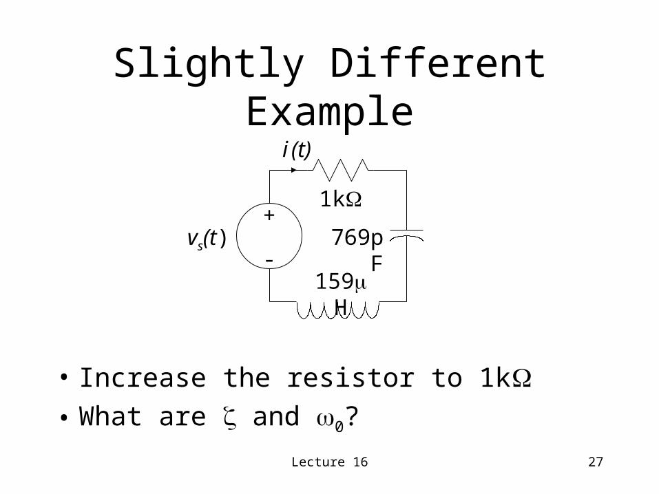
Slightly Different Example

• Increase the resistor to 1k• What are and 0?

1k+

-769pFvs(t)

i (t)

159H

Lecture 16 28

More Different Example

• = 2.2

• 0 = 2455000

• Is this system over damped, under damped, or critically damped?

• What will the current look like?

Lecture 16 29

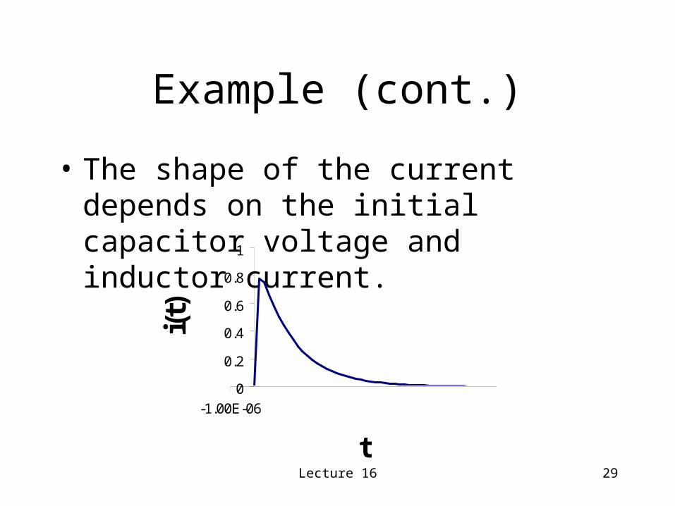
Example (cont.)

• The shape of the current depends on the initial capacitor voltage and inductor current.

0

0.2

0.4

0.6

0.8

1

-1.00E-06

t

i(t)