Lecture 15:The Tool-Narayanaswamy-Moynihan Equation Part II and DSC

March 9, 2010

Dr. Roger Loucks

Alfred UniversityDept. of Physics and Astronomy

loucks@alfred.edu

Thank you for taking me home !My eyes are completely open now ! I understand the glass transition very well !!!!

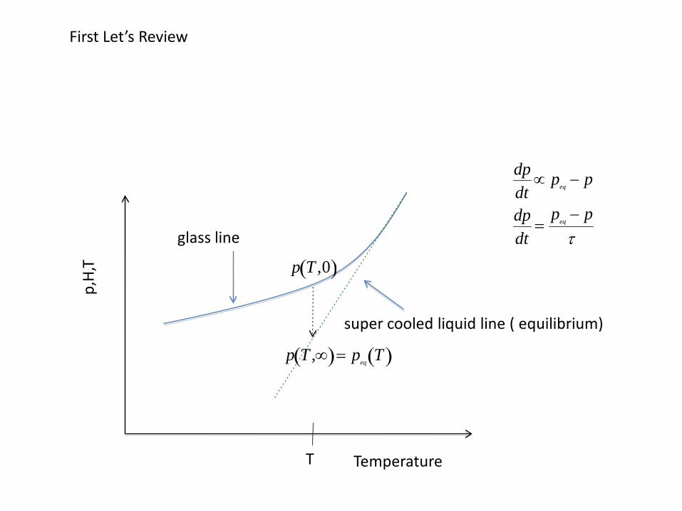
super cooled liquid line ( equilibrium)

glass line

p,H,

T

Temperature

p T ,0( )

p T ,∞( )= peq T( )

T

dpdt

∝ peq − p

dpdt

=peq − p

τ

First Let’s Review

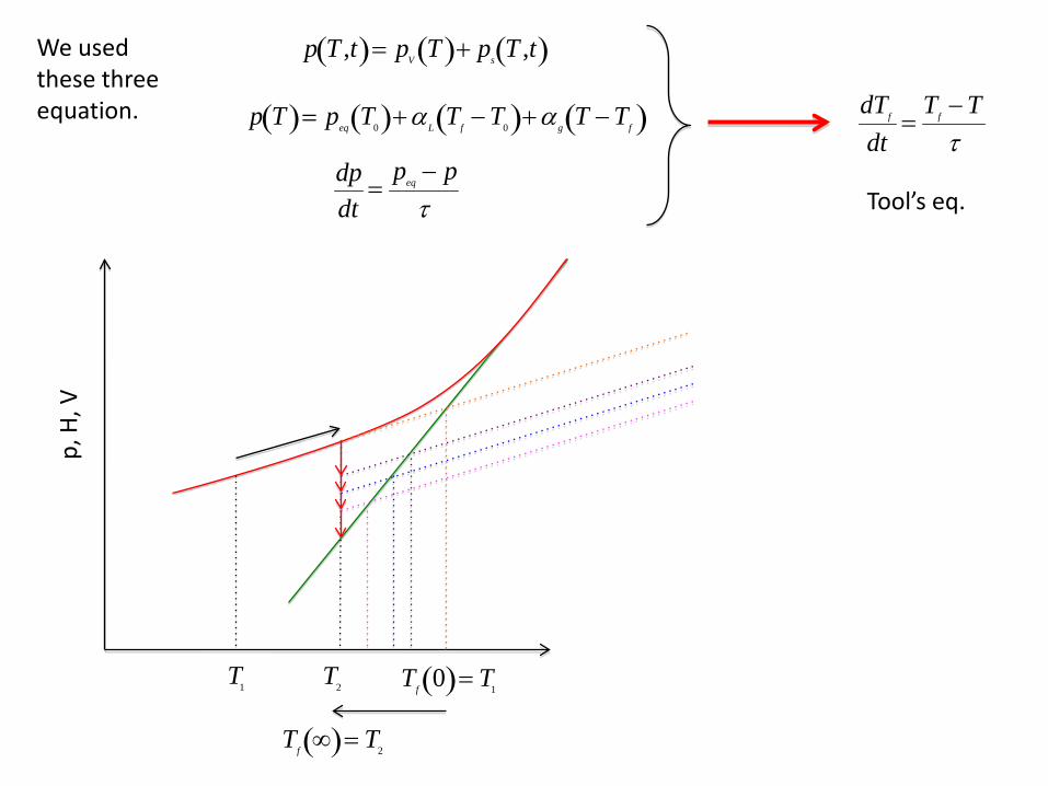
dTf

dt=

Tf − Tτ

Tool’s eq.

p T ,t( )= pV T( )+ ps T ,t( )

p T( )= peq T0( )+αL Tf − T0( )+αg T − Tf( )

We used these three equation.

dpdt

=peq − p

τ

Tf 0( )= T1

Tf ∞( )= T2

T1

p, H

, V

T2

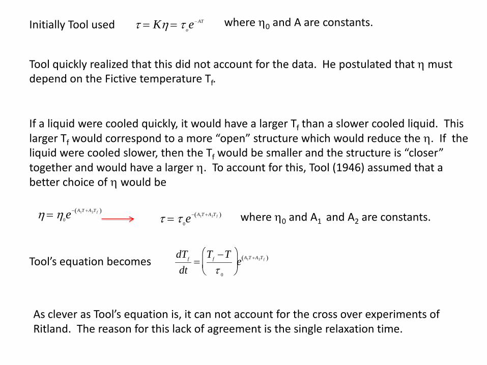
τ = Kη = τ oe− AT where η0 and A are constants.

Tool quickly realized that this did not account for the data. He postulated that η must depend on the Fictive temperature Tf.

If a liquid were cooled quickly, it would have a larger Tf than a slower cooled liquid. This larger Tf would correspond to a more “open” structure which would reduce the η. If the liquid were cooled slower, then the Tf would be smaller and the structure is “closer” together and would have a larger η. To account for this, Tool (1946) assumed that a better choice of η would be

η = η0e− A1T +A2T f( )

where η0 and A1 and A2 are constants.

τ = τ 0e− A1T +A2T f( )

Tool’s equation becomes

dTf

dt=

Tf −Tτ 0

e

A1T +A2T f( )

Initially Tool used

As clever as Tool’s equation is, it can not account for the cross over experiments of Ritland. The reason for this lack of agreement is the single relaxation time.

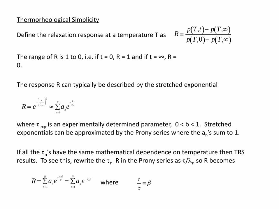
Thermorheological Simplicity

Define the relaxation response at a temperature T as

R ≡p T ,t( )− p T ,∞( )p T ,0( )− p T ,∞( )

The range of R is 1 to 0, i.e. if t = 0, R = 1 and if t = ∞, R = 0.

The response R can typically be described by the stretched exponential

R = e− t

τexp

b

≈ ann =1

N

∑ e− t

τn

where τexp is an experimentally determined parameter, 0 < b < 1. Stretched exponentials can be approximated by the Prony series where the an’s sum to 1.

If all the τn’s have the same mathematical dependence on temperature then TRS results. To see this, rewrite the τn R in the Prony series as τ/λn so R becomes

R = ann =1

N

∑ e−

λntτ = an

n =1

N

∑ e− λnβ

tτ

≡ βwhere

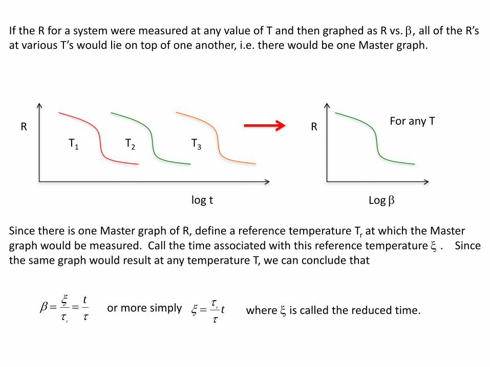
If the R for a system were measured at any value of T and then graphed as R vs. β, all of the R’s at various T’s would lie on top of one another, i.e. there would be one Master graph.

T1 T2 T3

log t

R For any T

Log β

R

Since there is one Master graph of R, define a reference temperature Tr at which the Master graph would be measured. Call the time associated with this reference temperature ξ . Since the same graph would result at any temperature T, we can conclude that

β = ξτ r

= tτ

or more simply

ξ = τ r

τt where ξ is called the reduced time.

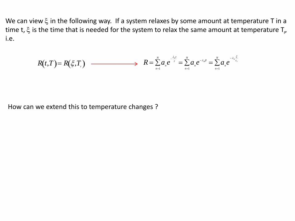
R t,T( )= R ξ,Tr( )

R = ann =1

N

∑ e−

λntτ = an

n =1

N

∑ e− λnβ = ann =1

N

∑ e− λn

ξτ r

We can view ξ in the following way. If a system relaxes by some amount at temperature T in a time t, ξ is the time that is needed for the system to relax the same amount at temperature Tr, i.e.

How can we extend this to temperature changes ?

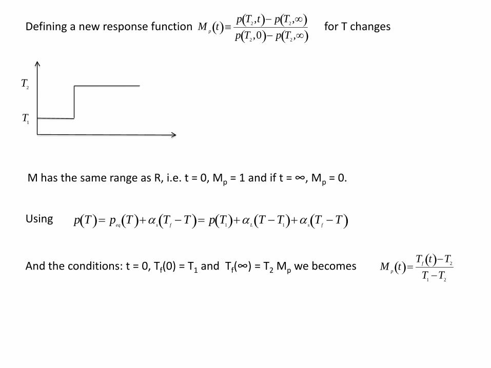
M p t( )≡p T2 ,t( )− p T2 ,∞( )p T2 ,0( )− p T2 ,∞( )

M has the same range as R, i.e. t = 0, Mp = 1 and if t = ∞, Mp = 0.

T1

T2

Defining a new response function for T changes

p T( )= peq T( )+αs Tf − T( )= p T1( )+αL T − T1( )+α s Tf − T( )Using

And the conditions: t = 0, Tf(0) = T1 and Tf(∞) = T2 Mp we becomes

M p t( )=Tf t( )−T2

T1 −T2

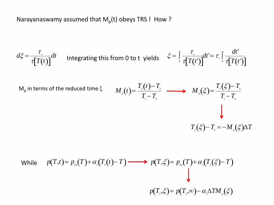
p T2 ,ξ( )= p T2 ,∞( )− αs∆TM p ξ( )

Tf ξ( )− T2 = −M p ξ( )∆T

p T ,t( )= peq T( )+α s Tf t( )− T( )

p T ,ξ( )= peq T( )+α s Tf ξ( )− T( )

M p t( )=Tf t( )− T2

T1 − T2

Mp in terms of the reduced time ξ

dξ = τ r

τ T t( )[ ]dt Integrating this from 0 to t yields

ξ = τ r

τ T t'( )[ ]0

t

∫ dt '= τ r

dt'τ T t '( )[ ]0

t

∫

M p ξ( )=Tf ξ( )− T2

T1 − T2

Narayanaswamy assumed that Mp(t) obeys TRS ! How ?

While

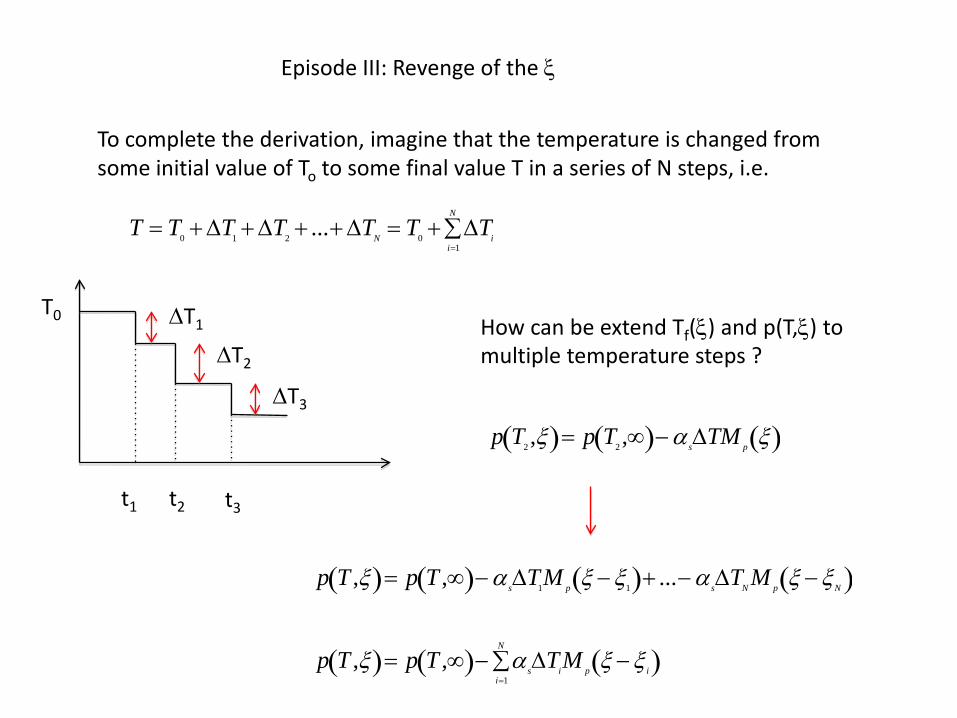
Episode III: Revenge of the ξ

p T2 ,ξ( )= p T2 ,∞( )− αs∆TM p ξ( )

To complete the derivation, imagine that the temperature is changed from some initial value of To to some final value T in a series of N steps, i.e.

T = T0 + ∆T1 + ∆T2 + ...+ ∆TN = T0 + ∆Tii=1

N

∑

∆T1

∆T2

∆T3

T0

t1 t2 t3

How can be extend Tf(ξ) and p(T,ξ) to multiple temperature steps ?

p T ,ξ( )= p T ,∞( )− αs∆T1M p ξ − ξ1( )+ ...− α s∆TN M p ξ − ξN( )

p T ,ξ( )= p T ,∞( )− αs∆TiM p ξ − ξ i( )i=1

N

∑

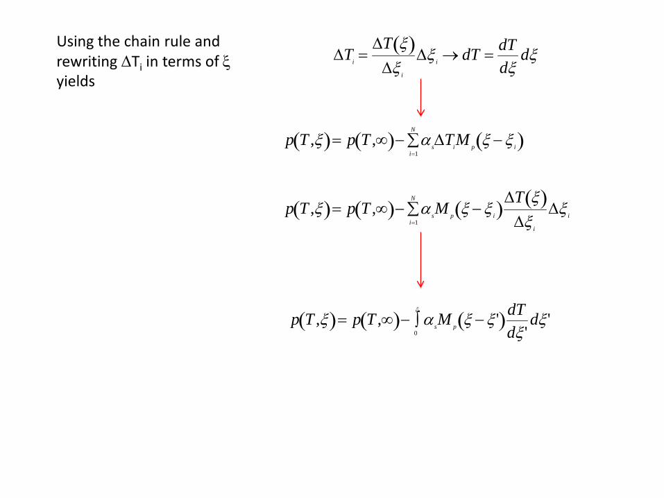
p T ,ξ( )= p T ,∞( )− αsM p ξ − ξ '( )0

ξ

∫dTdξ '

dξ '

Using the chain rule and rewriting ∆Ti in terms of ξyields

p T ,ξ( )= p T ,∞( )− αs∆TiM p ξ − ξ i( )i=1

N

∑

p T ,ξ( )= p T ,∞( )− αsM p ξ − ξ i( )i=1

N

∑∆T ξ( )

∆ξ i

∆ξ i

∆Ti =∆T ξ( )

∆ξ i

∆ξ i → dT = dTdξ

dξ

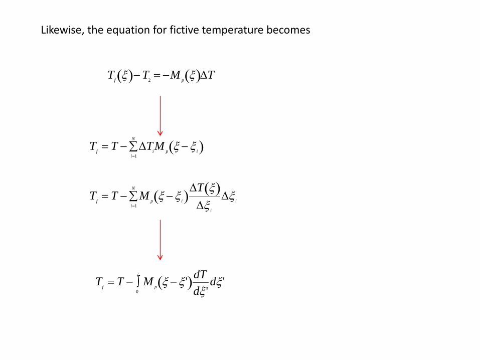
Likewise, the equation for fictive temperature becomes

Tf ξ( )− T2 = −M p ξ( )∆T

Tf = T − ∆TiM p ξ − ξ i( )i=1

N

∑

Tf = T − M p ξ − ξ i( )i=1

N

∑∆T ξ( )

∆ξ i

∆ξ i

Tf = T − M p ξ − ξ '( )0

ξ

∫dTdξ '

dξ '

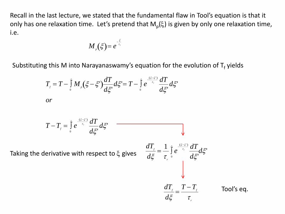
Recall in the last lecture, we stated that the fundamental flaw in Tool’s equation is that it only has one relaxation time. Let’s pretend that Mp(ξ) is given by only one relaxation time, i.e.

M p ξ( )= e− ξ

τ r

Tf = T − M p ξ − ξ '( )0

ξ

∫dTdξ '

dξ '= T − e−

ξ −ξ '( )τ r

0

ξ

∫dTdξ '

dξ '

or

T − Tf = e−

ξ −ξ '( )τ r

0

ξ

∫dTdξ '

dξ '

Substituting this M into Narayanaswamy’s equation for the evolution of Tf yields

Taking the derivative with respect to ξ gives

dTf

dξ= 1

τ r

e−

ξ −ξ '( )τ r

dTdξ '0

ξ

∫ dξ '

dTf

dξ=

T − Tf

τ r

Tool’s eq.

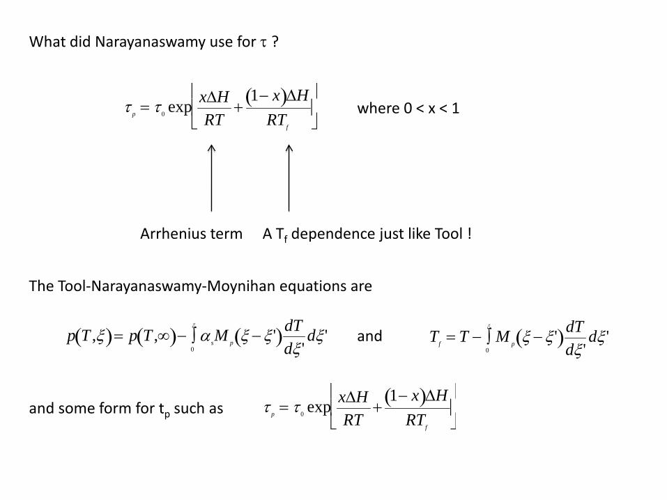
What did Narayanaswamy use for τ ?

τ p = τ 0 exp x∆HRT

+1− x( )∆H

RTf

Arrhenius term A Tf dependence just like Tool !

p T ,ξ( )= p T ,∞( )− αsM p ξ − ξ '( )0

ξ

∫dTdξ '

dξ '

The Tool-Narayanaswamy-Moynihan equations are

and

Tf = T − M p ξ − ξ '( )0

ξ

∫dTdξ '

dξ '

and some form for tp such as

τ p = τ 0 exp x∆HRT

+1− x( )∆H

RTf

where 0 < x < 1

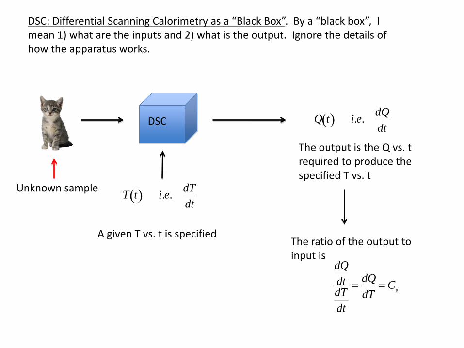
DSC: Differential Scanning Calorimetry as a “Black Box”. By a “black box”, I mean 1) what are the inputs and 2) what is the output. Ignore the details of how the apparatus works.

DSC

Unknown sample

T t( ) i.e. dTdt

A given T vs. t is specified

The output is the Q vs. t required to produce the specified T vs. t

Q t( ) i.e. dQdt

The ratio of the output to input is

dQdtdTdt

= dQdT

= Cp

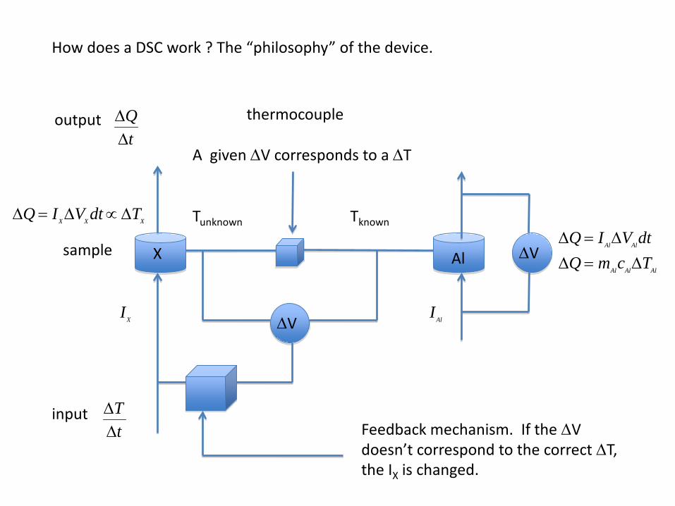
How does a DSC work ? The “philosophy” of the device.

X Al

thermocouple

A given ∆V corresponds to a ∆T

∆V

TknownTunknown

∆V

∆Q = IAl∆VAldt∆Q = mAlcAl∆TAl

∆Q = IX ∆VX dt ∝ ∆TX

IAl

IX

Feedback mechanism. If the ∆V doesn’t correspond to the correct ∆T, the IX is changed.

∆Q∆t

output

input

∆T∆t

sample

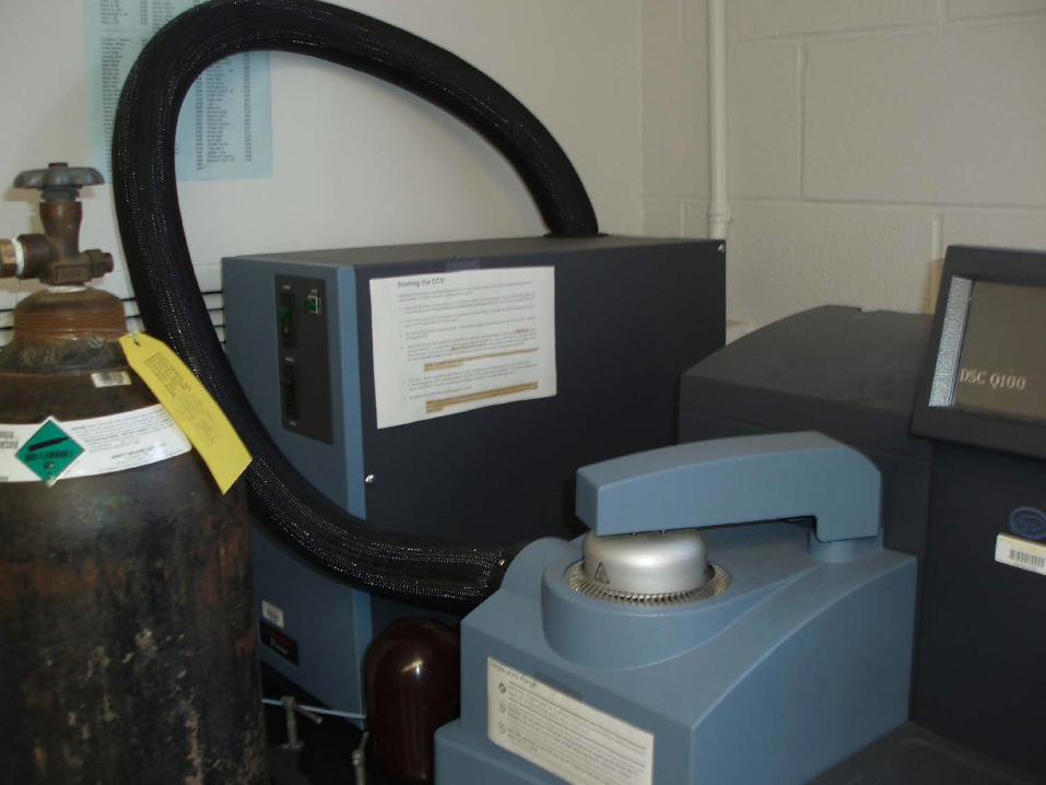
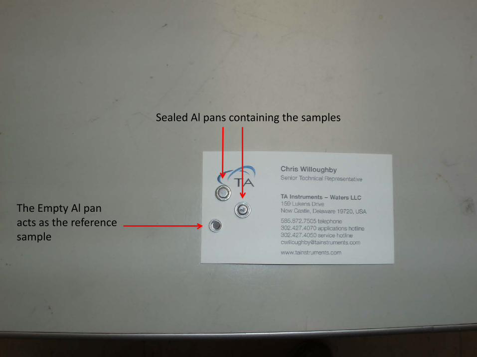
The Empty Al pan acts as the reference sample

Sealed Al pans containing the samples

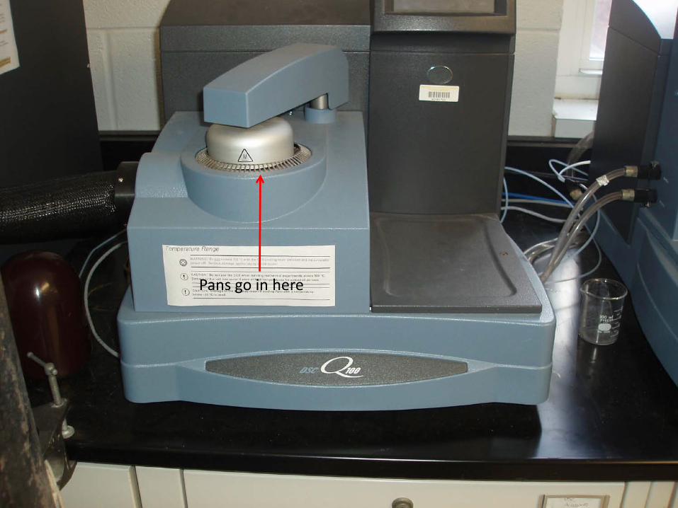
Pans go in here

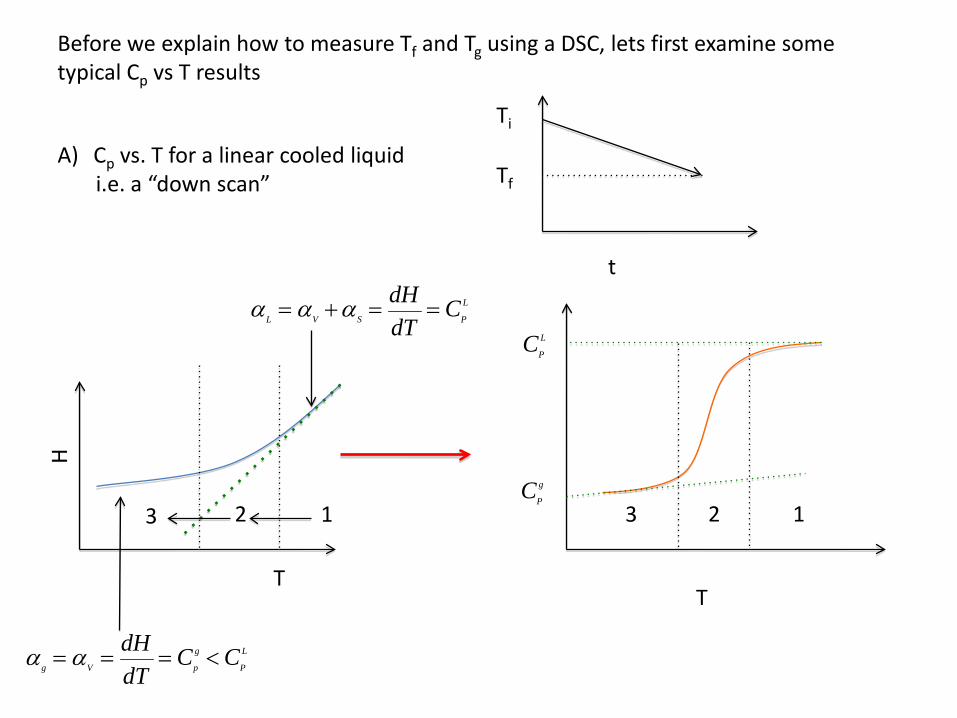
Before we explain how to measure Tf and Tg using a DSC, lets first examine some typical Cp vs T results

A) Cp vs. T for a linear cooled liquidi.e. a “down scan”

Ti

Tf

t

T

H

αg = αV = dHdT

= Cp

g < CP

L

αL = αV +αS = dHdT

= CP

L

T

2 13 123

CP

L

CP

g

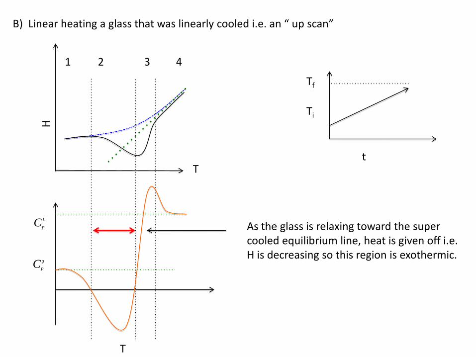
B) Linear heating a glass that was linearly cooled i.e. an “ up scan”

Ti

Tf

tT

H

T

21 4

CP

L

CP

g

3

As the glass is relaxing toward the super cooled equilibrium line, heat is given off i.e. H is decreasing so this region is exothermic.

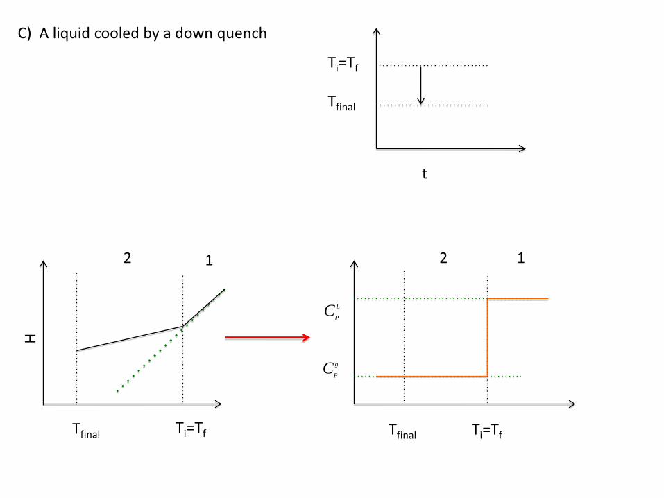
C) A liquid cooled by a down quench

Ti=Tf

Tfinal

t

H

2 1

CP

L

CP

g

Ti=TfTfinal

12

Tfinal Ti=Tf

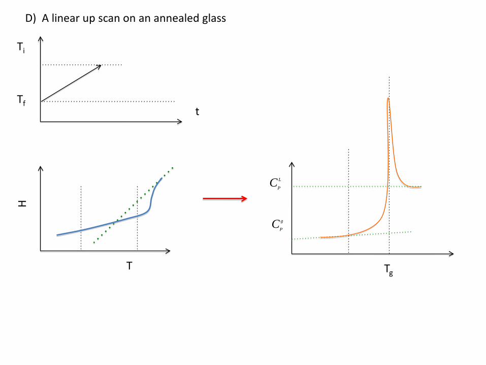
D) A linear up scan on an annealed glass

Ti

t

T

H

Tf

Tg

CP

L

CP

g

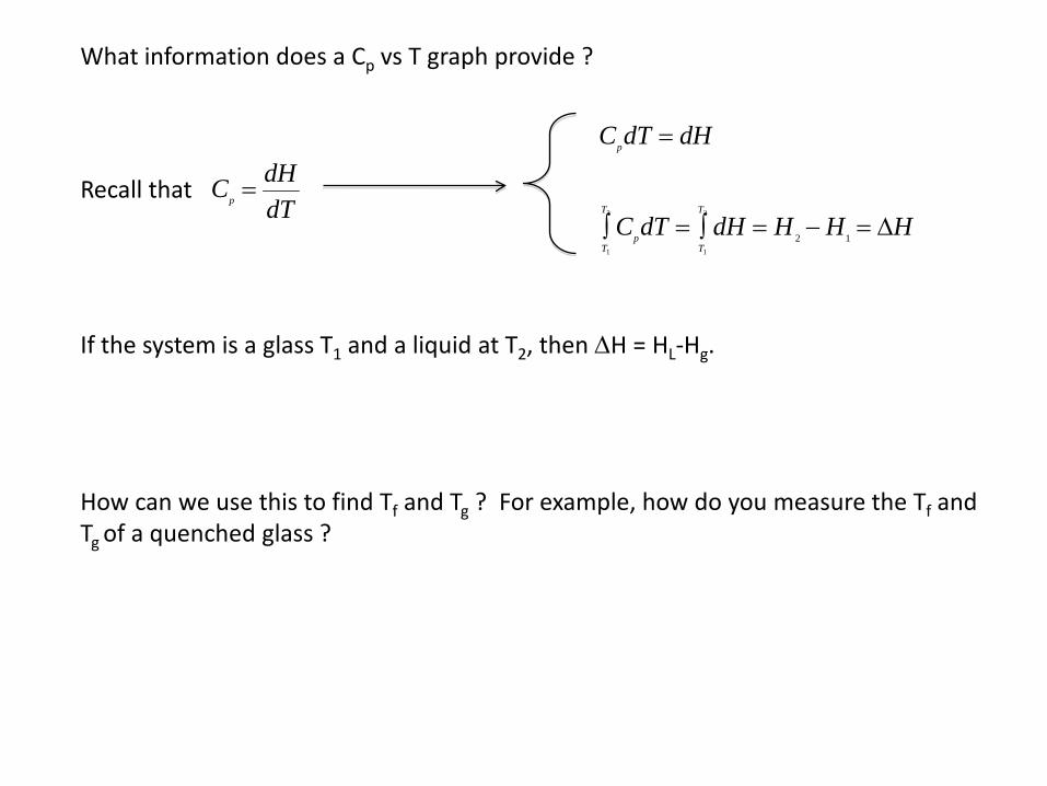
What information does a Cp vs T graph provide ?

Recall that

Cp = dHdT

CpdT = dH

CpT1

T2

∫ dT = dHT1

T2

∫ = H 2 − H1 = ∆H

How can we use this to find Tf and Tg ? For example, how do you measure the Tf and Tg of a quenched glass ?

If the system is a glass T1 and a liquid at T2, then ∆H = HL-Hg.

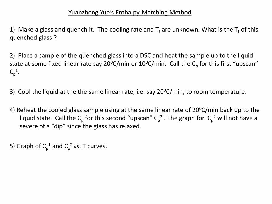
1) Make a glass and quench it. The cooling rate and Tf are unknown. What is the Tf of this quenched glass ?

2) Place a sample of the quenched glass into a DSC and heat the sample up to the liquid state at some fixed linear rate say 200C/min or 100C/min. Call the Cp for this first “upscan” Cp

1.

3) Cool the liquid at the the same linear rate, i.e. say 200C/min, to room temperature.

4) Reheat the cooled glass sample using at the same linear rate of 200C/min back up to the liquid state. Call the Cp for this second “upscan” Cp

2 . The graph for Cp2 will not have a

severe of a “dip” since the glass has relaxed.

5) Graph of Cp1 and Cp

2 vs. T curves.

Yuanzheng Yue’s Enthalpy-Matching Method

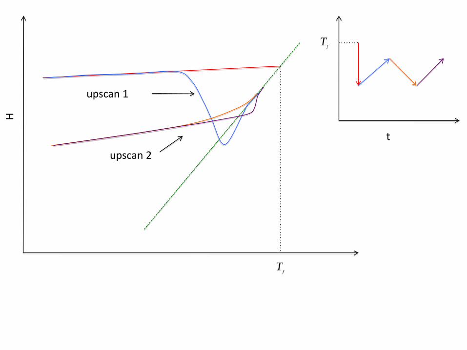
Tf

Tf

t

H

upscan 1

upscan 2

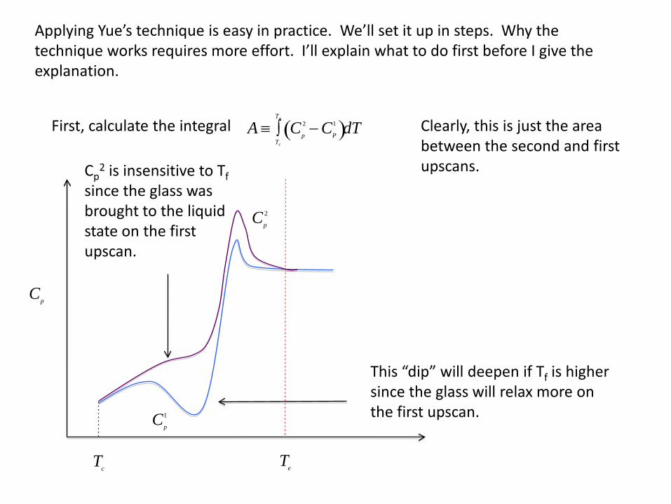
A ≡ Cp

2 − CP

1( )Tc

Tg

∫ dT

Applying Yue’s technique is easy in practice. We’ll set it up in steps. Why the technique works requires more effort. I’ll explain what to do first before I give the explanation.

First, calculate the integral Clearly, this is just the area between the second and first upscans.

Cp

1

Cp

2

Cp

Tc

Te

This “dip” will deepen if Tf is higher since the glass will relax more on the first upscan.

Cp2 is insensitive to Tf

since the glass was brought to the liquid state on the first upscan.

Cp

1

Cp

2

Cp

Cp ,L

Cp ,g

TG

Tf

Tc

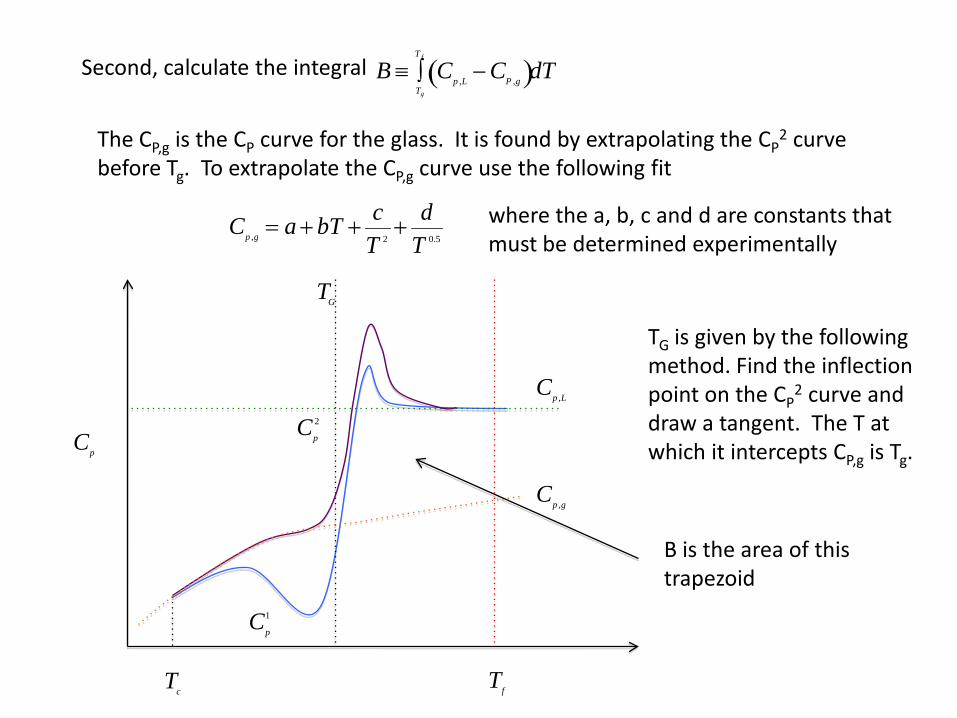
B ≡ Cp ,L − CP ,g( )Tg

T f

∫ dTSecond, calculate the integral

The CP,g is the CP curve for the glass. It is found by extrapolating the CP2 curve

before Tg. To extrapolate the CP,g curve use the following fit

Cp ,g = a + bT + cT 2

+ dT 0.5

where the a, b, c and d are constants that must be determined experimentally

TG is given by the following method. Find the inflection point on the CP

2 curve and draw a tangent. The T at which it intercepts CP,g is Tg.

B is the area of this trapezoid

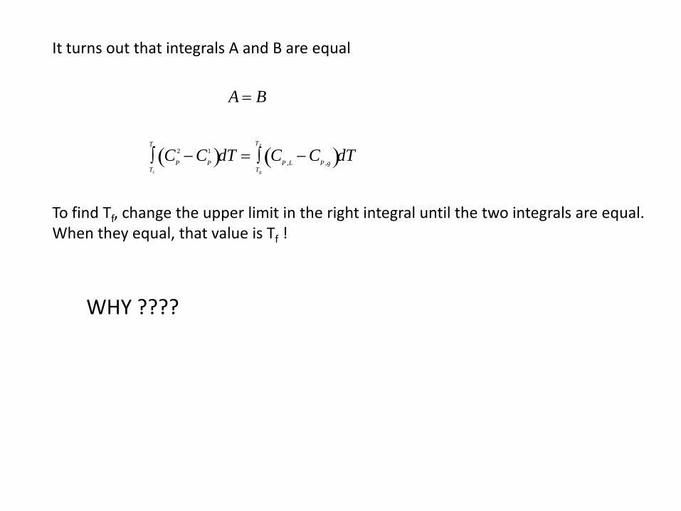
It turns out that integrals A and B are equal

A = B

CP

2 − CP

1( )Tc

Te

∫ dT = CP ,L − CP ,g( )Tg

T f

∫ dT

To find Tf, change the upper limit in the right integral until the two integrals are equal. When they equal, that value is Tf !

WHY ????

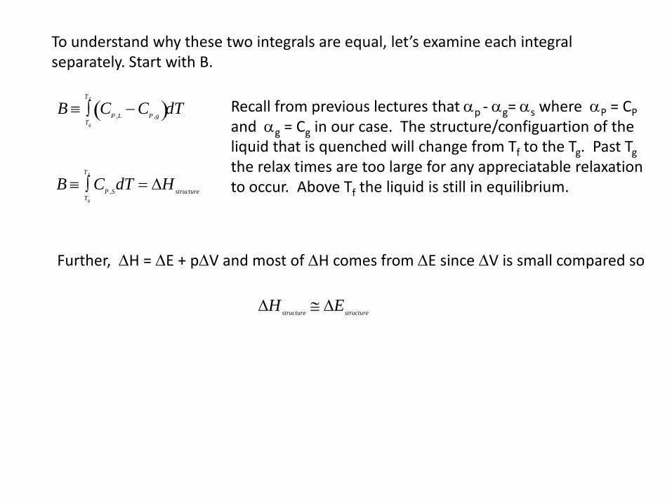
To understand why these two integrals are equal, let’s examine each integral separately. Start with B.

B ≡ CP ,L − CP ,g( )Tg

T f

∫ dT Recall from previous lectures that αp - αg= αs where αP = CPand αg = Cg in our case. The structure/configuartion of the liquid that is quenched will change from Tf to the Tg. Past Tgthe relax times are too large for any appreciatable relaxation to occur. Above Tf the liquid is still in equilibrium.

Further, ∆H = ∆E + p∆V and most of ∆H comes from ∆E since ∆V is small compared so

B ≡ CP ,SdT = ∆HstructureTg

T f

∫

∆Hstructure ≅ ∆Estructure

Now let’s consider the left integral A.

A ≡ Cp

2 − CP

1( )Tc

Te

∫ dTBelow Tc both Cp

1 and CP2 are identical. Recall that the slopes of p vs

T graphs for low T were all identical ! Above Te, both Cp1 and CP

2 are identical since they are in the both liquids.

The vibrational contributional to Cp1 and Cp

2 are identical at a given T. Therefore, the vibrational contributions cancel and all that is left is the contribution from structural changes. Note that if the upper limit of this integral was extended to Tf, the integral would not since Cp

1 = CP2 in the liquid region.

Therefore, A is also equal to ∆Hstructure.

∴ A = B Yue is very clever !

This is an active area of work !!!!!!!