Embed Size (px)
Citation preview

THEORY OF COMPILATIONLecture 15 – Dataflow Analysis
Eran Yahav
www.cs.technion.ac.il/~yahave/tocs2011/compilers-lec15.pptx

2
Static Analysis
Reason statically (at compile time) about the possible runtime behaviors of a program
“The algorithmic discovery of properties of a program by inspection of its source text1”-- Manna, Pnueli
1 Does not have to literally be the source text, just means w/o running it
3
Static Analysis
x = ?if (x > 0) { y = 42;} else { y = 73; foo();} assert (y == 42);
Bad news: problem is generally undecidable
4
universe
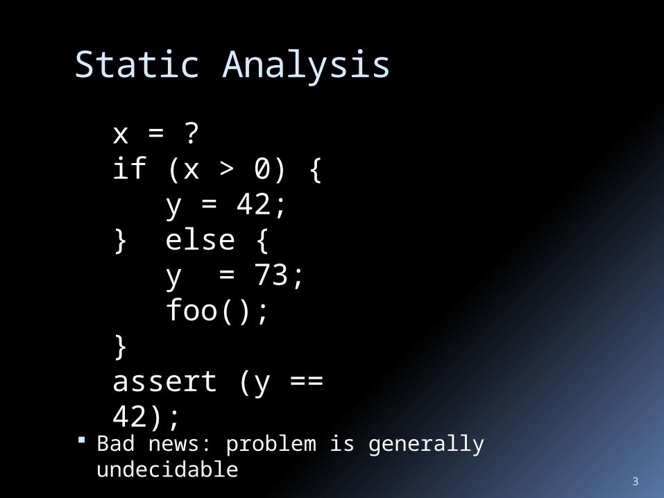
Static Analysis
Central idea: use approximation
Under Approximation
Exact set of configurations/behaviors
Over Approximation
5
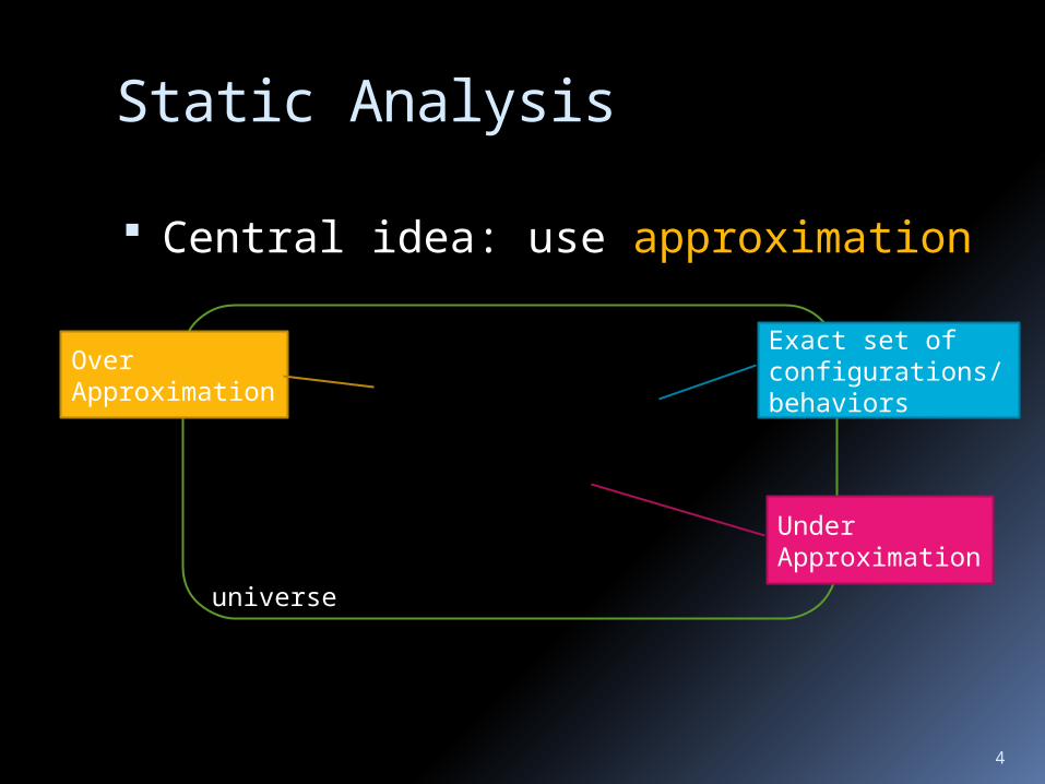
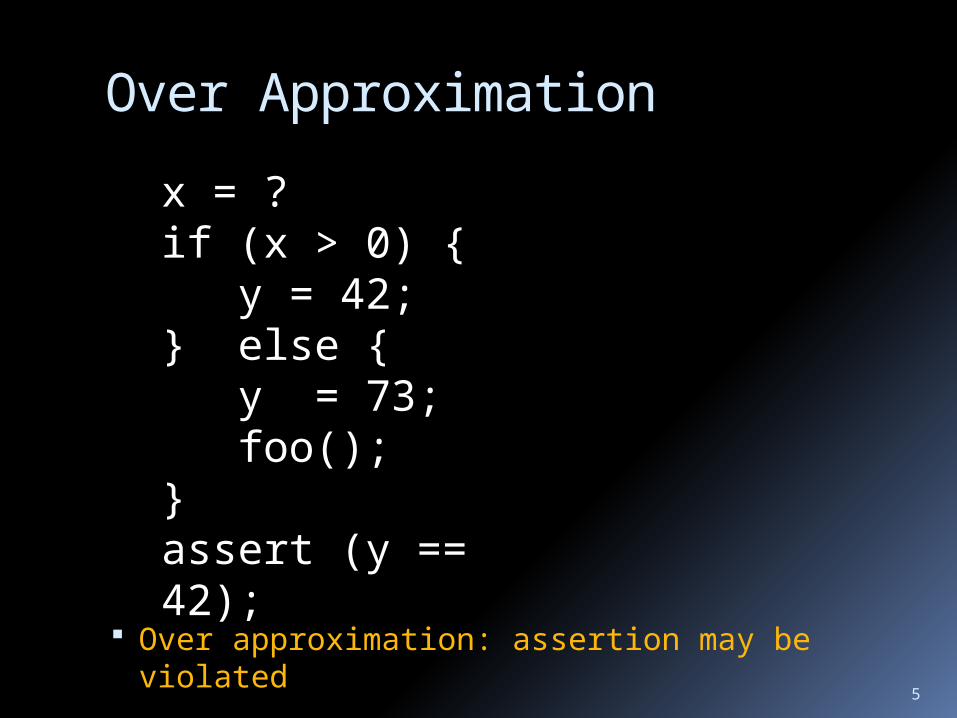
Over Approximation
x = ?if (x > 0) { y = 42;} else { y = 73; foo();} assert (y == 42);
Over approximation: assertion may be violated
6
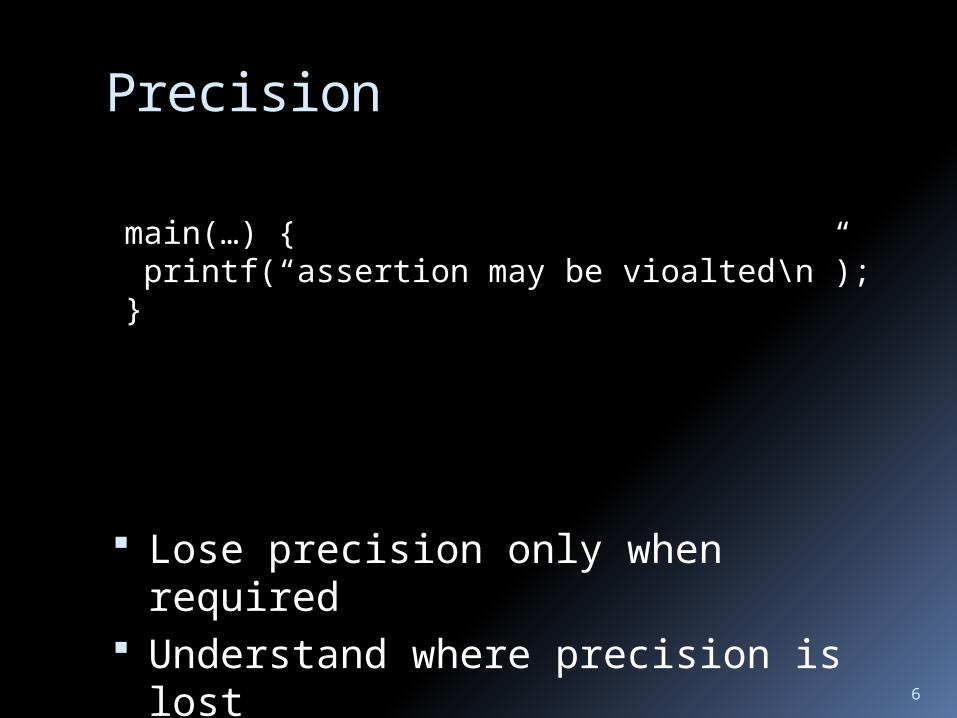
Lose precision only when required Understand where precision is lost
Precision
main(…) { printf(“assertion may be vioalted\n”);}
7
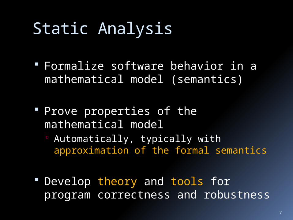
Static Analysis
Formalize software behavior in a mathematical model (semantics)
Prove properties of the mathematical model Automatically, typically with approximation
of the formal semantics
Develop theory and tools for program correctness and robustness
8
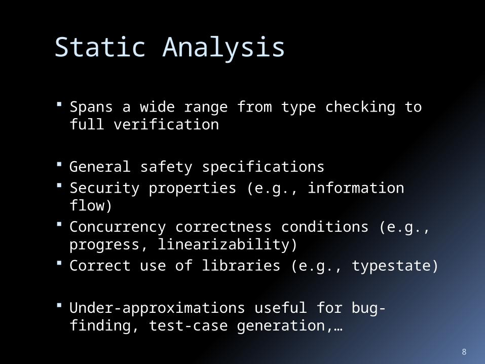
Static Analysis
Spans a wide range from type checking to full verification
General safety specifications Security properties (e.g., information flow) Concurrency correctness conditions (e.g.,
progress, linearizability) Correct use of libraries (e.g., typestate)
Under-approximations useful for bug-finding, test-case generation,…

9
Static Analysis: Techniques Dataflow analysis Constraint-based analysis Type and effect systems Abstract Interpretation
(advanced course next semester) …
10
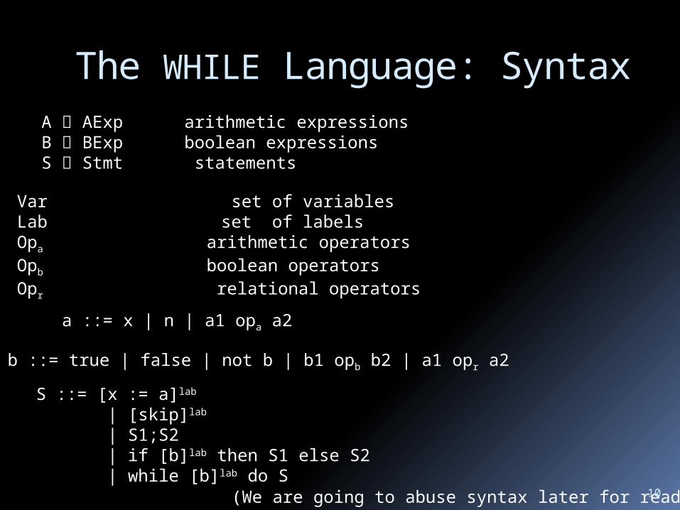
The WHILE Language: SyntaxA AExp arithmetic expressionsB BExp boolean expressionsS Stmt statements
Var set of variablesLab set of labelsOpa arithmetic operatorsOpb boolean operatorsOpr relational operators
a ::= x | n | a1 opa a2
b ::= true | false | not b | b1 opb b2 | a1 opr a2
S ::= [x := a]lab | [skip]lab
| S1;S2 | if [b]lab then S1 else S2 | while [b]lab do S
(We are going to abuse syntax later for readability)
11
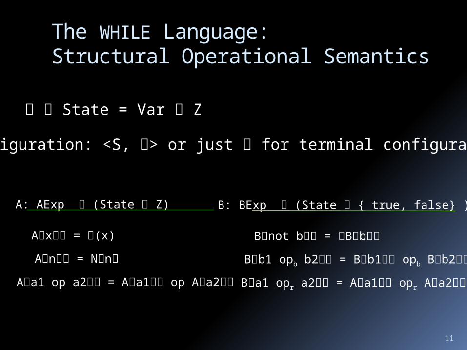
A: AExp (State Z)
Ax = (x)
An = Nn
Aa1 op a2 = Aa1 op Aa2
B: BExp (State { true, false} )
Bnot b = Bb
Bb1 opb b2 = Bb1 opb Bb2
Ba1 opr a2 = Aa1 opr Aa2
State = Var Z
The WHILE Language: Structural Operational Semantics
Configuration: <S, > or just for terminal configuration
12
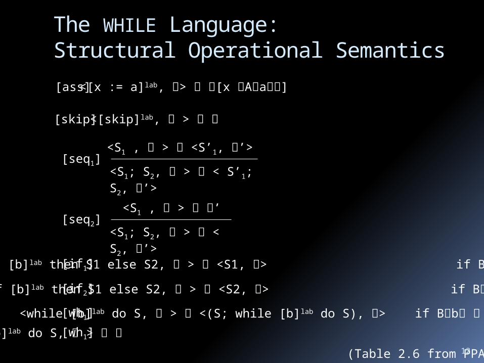
The WHILE Language: Structural Operational Semantics
(Table 2.6 from PPA)
[seq1] <S1 , > <S’1, ’>
<S1; S2, > < S’1; S2, ’>
[seq2] <S1 , > ’
<S1; S2, > < S2, ’>
<[x := a]lab, > [x Aa][ass]
<[skip]lab, > [skip]
<if [b]lab then S1 else S2, > <S1, > if Bb = true[if1]
<if [b]lab then S1 else S2, > <S2, > if Bb = false[if2]
<while [b]lab do S, > <(S; while [b]lab do S), > if Bb = true[wh1]
<while [b]lab do S, > if Bb = false[wh1]
13
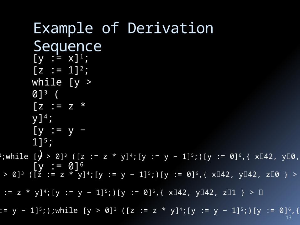
Example of Derivation Sequence[y := x]1;[z := 1]2;while [y > 0]3 ([z := z * y]4;[y := y − 1]5; )[y := 0]6
< [y := x]1;[z := 1]2;while [y > 0]3 ([z := z * y]4;[y := y − 1]5;)[y := 0]6,{ x42, y0, z0 } >
< [z := 1]2;while [y > 0]3 ([z := z * y]4;[y := y − 1]5;)[y := 0]6,{ x42, y42, z0 } >
< while [y > 0]3 ([z := z * y]4;[y := y − 1]5;)[y := 0]6,{ x42, y42, z1 } >
< ([z := z * y]4;[y := y − 1]5;);while [y > 0]3 ([z := z * y]4;[y := y − 1]5;)[y := 0]6,{ x42, y42, z1 }> …
14
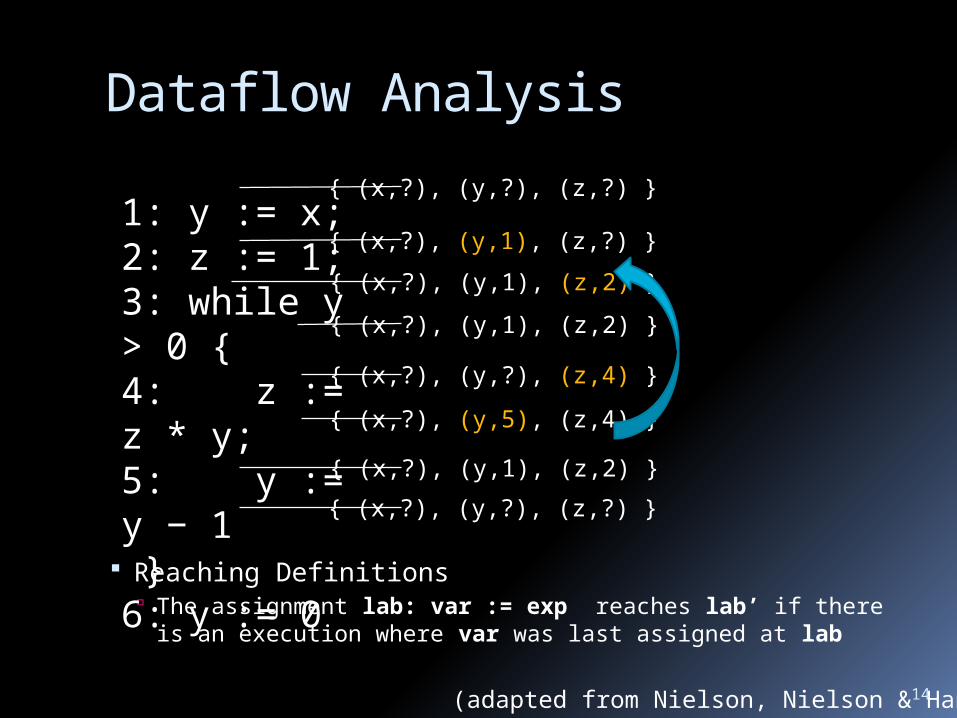
Dataflow Analysis
Reaching Definitions The assignment lab: var := exp reaches lab’ if there
is an execution where var was last assigned at lab
1: y := x;2: z := 1;3: while y > 0 {4: z := z * y;5: y := y − 1 }6: y := 0
(adapted from Nielson, Nielson & Hankin)
{ (x,?), (y,?), (z,?) }
{ (x,?), (y,1), (z,?) }
{ (x,?), (y,1), (z,2) }
{ (x,?), (y,?), (z,4) }
{ (x,?), (y,5), (z,4) }
{ (x,?), (y,1), (z,2) }
{ (x,?), (y,?), (z,?) }
{ (x,?), (y,1), (z,2) }
15
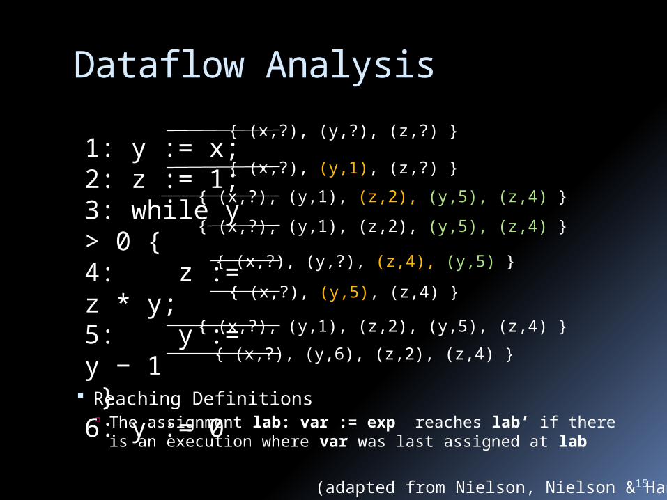
Dataflow Analysis
Reaching Definitions The assignment lab: var := exp reaches lab’ if there
is an execution where var was last assigned at lab
1: y := x;2: z := 1;3: while y > 0 {4: z := z * y;5: y := y − 1 }6: y := 0
(adapted from Nielson, Nielson & Hankin)
{ (x,?), (y,?), (z,?) }
{ (x,?), (y,1), (z,?) }
{ (x,?), (y,1), (z,2), (y,5), (z,4) }
{ (x,?), (y,?), (z,4), (y,5) }
{ (x,?), (y,5), (z,4) }
{ (x,?), (y,1), (z,2), (y,5), (z,4) }
{ (x,?), (y,6), (z,2), (z,4) }
{ (x,?), (y,1), (z,2), (y,5), (z,4) }
16
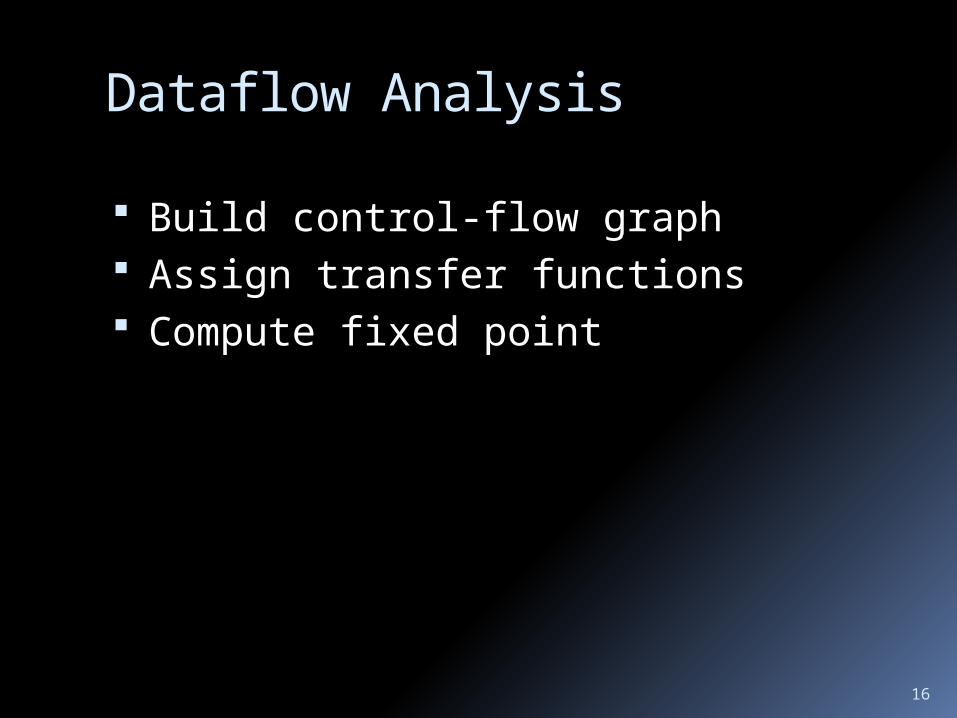
Dataflow Analysis
Build control-flow graph Assign transfer functions Compute fixed point
17
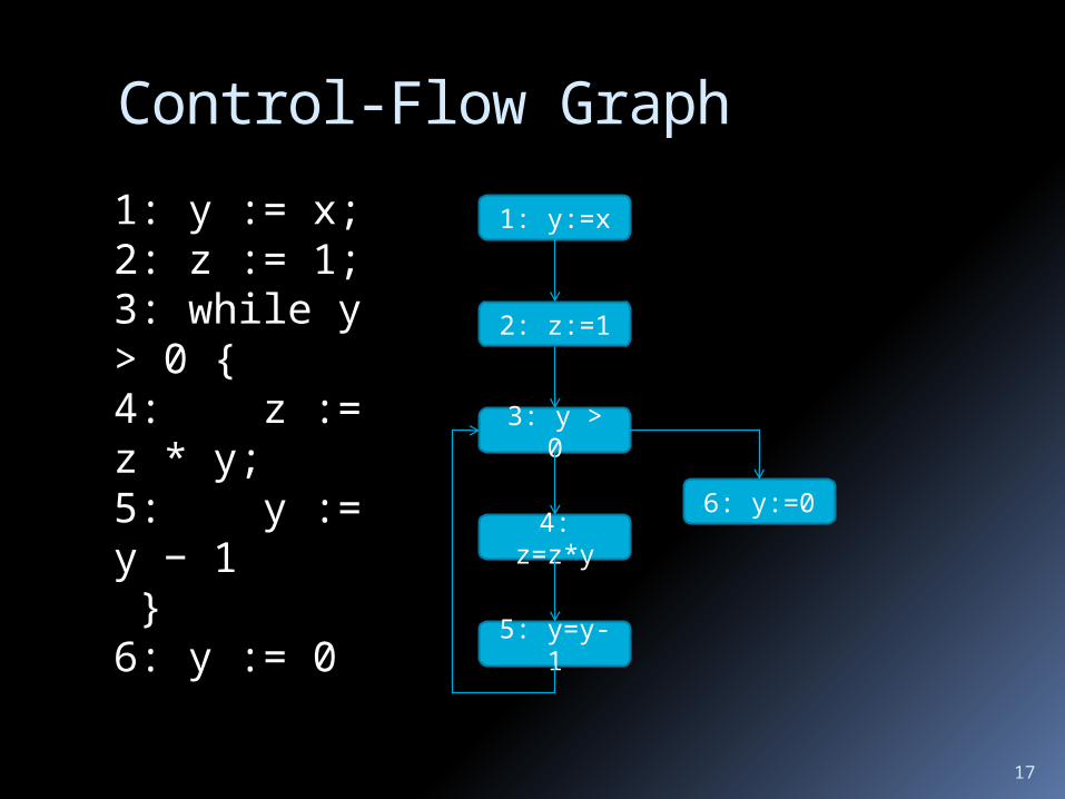
Control-Flow Graph
1: y := x;2: z := 1;3: while y > 0 {4: z := z * y;5: y := y − 1 }6: y := 0
1: y:=x
2: z:=1
3: y > 0
4: z=z*y
5: y=y-1
6: y:=0
18
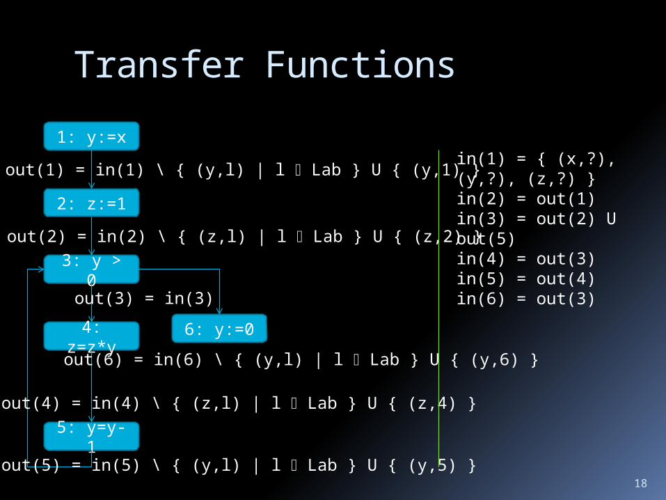
Transfer Functions
1: y:=x
2: z:=1
3: y > 0
4: z=z*y
5: y=y-1
6: y:=0
out(1) = in(1) \ { (y,l) | l Lab } U { (y,1) }
out(2) = in(2) \ { (z,l) | l Lab } U { (z,2) }
in(1) = { (x,?), (y,?), (z,?) } in(2) = out(1)in(3) = out(2) U out(5)in(4) = out(3)in(5) = out(4)in(6) = out(3)
out(4) = in(4) \ { (z,l) | l Lab } U { (z,4) }
out(5) = in(5) \ { (y,l) | l Lab } U { (y,5) }
out(6) = in(6) \ { (y,l) | l Lab } U { (y,6) }
out(3) = in(3)
19
System of Equationsin(1) = { (x,?), (y,?), (z,?) } in(2) = out(1)in(3) = out(2) U out(5)in(4) = out(3)in(5) = out(4)In(6) = out(3)out(1) = in(1) \ { (y,l) | l Lab } U { (y,1) }out(2) = in(2) \ { (z,l) | l Lab } U { (z,2) }out(3) = in(3)out(4) = in(4) \ { (z,l) | l Lab } U { (z,4) }out(5) = in(5) \ { (y,l) | l Lab } U { (y,5) }out(6) = in(6) \ { (y,l) | l Lab } U { (y,6) }F: ((Var x Lab) )12 ((Var x Lab) )12

20
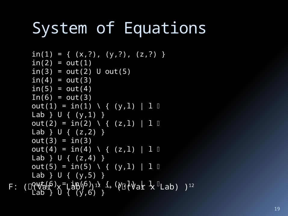
System of Equations
in(1) = { (x,?), (y,?), (z,?) } in(2) = out(1)in(3) = out(2) U out(5)in(4) = out(3)in(5) = out(4)In(6) = out(3)out(1) = in(1) \ { (y,l) | l Lab } U { (y,1) }out(2) = in(2) \ { (z,l) | l Lab } U { (z,2) }out(3) = in(3)out(4) = in(4) \ { (z,l) | l Lab } U { (z,4) }out(5) = in(5) \ { (y,l) | l Lab } U { (y,5) }out(6) = in(6) \ { (y,l) | l Lab } U { (y,6) }
F: ((Var x Lab) )12 ((Var x Lab) )12
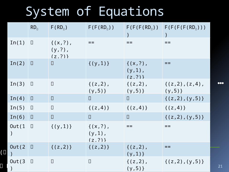
in(1)={(x,?),(y,?),(z,?)} , in(2)=out(1), in(3)=out(2) U out(5), in(4)=out(3), in(5)=out(4),In(6) = out(3)out(1) = in(1) \ { (y,l) | l Lab } U { (y,1) }, out(2) = in(2) \ { (z,l) | l Lab } U { (z,2) }out(3) = in(3), out(4) = in(4) \ { (z,l) | l Lab } U { (z,4) }out(5) = in(5) \ { (y,l) | l Lab } U { (y,5) }, out(6) = in(6) \ { (y,l) | l Lab } U { (y,6) }
In(1) {(x,?),(y,?),(z,?)}
== == ==
In(2) {(y,1)} {(x,?),(y,1),(z,?)}
==
In(3) {(z,2),(y,5)} {(z,2),(y,5)} {(z,2),(z,4),(y,5)}
In(4) {(z,2),(y,5)}
In(5) {(z,4)} {(z,4)} {(z,4)}
In(6) {(z,2),(y,5)}
Out(1)
{(y,1)} {(x,?),(y,1),(z,?)}
== ==
Out(2)
{(z,2)} {(z,2)} {(z,2),(y,1)} ==
Out(3)
{(z,2),(y,5)} {(z,2),(y,5)}
Out(4)
{(z,4)} {(z,4)} {(z,4)} {(z,4)}
Out(5)
{(y,5)} {(y,5)} {(z,4),(y,5)} {(z,4),(y,5)}
Out(6)
{(y,6)} {(y,6)} {(y,6)} {(y,6)}
…
21
F: ((Var x Lab) )12 ((Var x Lab) )12
RD RD’ when i: RD(i) RD’(i)
…
RD F(RD) F(F(RD)) F(F(F(RD))) F(F(F(F(RD))))
In(1) {(x,?),(y,?),(z,?)}
== == ==
In(2) {(y,1)} {(x,?),(y,1),(z,?)}
==
In(3) {(z,2),(y,5)} {(z,2),(y,5)} {(z,2),(z,4),(y,5)}
In(4) {(z,2),(y,5)}
In(5) {(z,4)} {(z,4)} {(z,4)}
In(6) {(z,2),(y,5)}
Out(1)
{(y,1)} {(x,?),(y,1),(z,?)}
== ==
Out(2)
{(z,2)} {(z,2)} {(z,2),(y,1)} ==
Out(3)
{(z,2),(y,5)} {(z,2),(y,5)}
Out(4)
{(z,4)} {(z,4)} {(z,4)} {(z,4)}
Out(5)
{(y,5)} {(y,5)} {(z,4),(y,5)} {(z,4),(y,5)}
Out(6)
{(y,6)} {(y,6)} {(y,6)} {(y,6)}
System of Equations
22
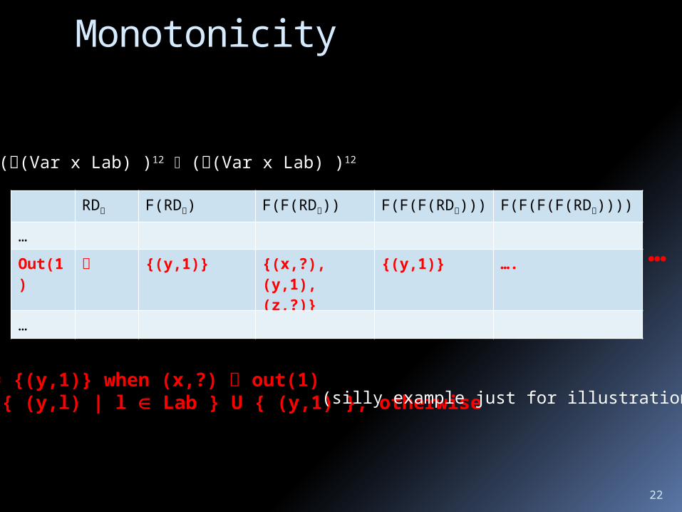
Monotonicity
F: ((Var x Lab) )12 ((Var x Lab) )12
RD F(RD) F(F(RD)) F(F(F(RD))) F(F(F(F(RD))))
…
Out(1)
{(y,1)} {(x,?),(y,1),(z,?)}
{(y,1)} ….
…
…
out(1) = {(y,1)} when (x,?) out(1)in(1) \ { (y,l) | l Lab } U { (y,1) }, otherwise(silly example just for illustration)
23
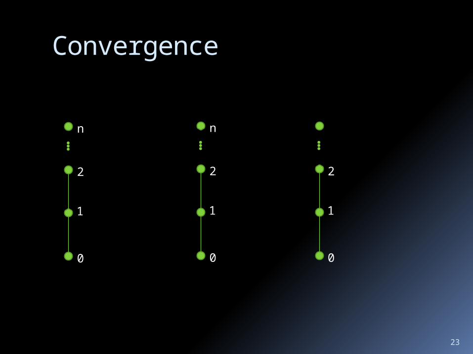
Convergence
0
1…
2
n
0
1
…
2
n
0
1
…
2

24
Least Fixed Point
We will see later why it exists For now, mostly informally…F: ((Var x Lab) )12 ((Var x Lab) )12
RD RD’ when i: RD(i) RD’(i)
F is monotone: RD RD’ implies that F(RD) F(RD’)
RD = (, ,…,)
F(RD), F(F(RD) , F(F(F(RD)), … Fn(RD)
Fn+1(RD) = Fn(RD)
RD
F(RD)
F(F(RD))
…
Fn(RD)

25
Things that Should Trouble You
How did we get the transfer functions?
How do we know these transfer functions are safe (conservative)?
How do we know that these transfer functions are optimal?
26
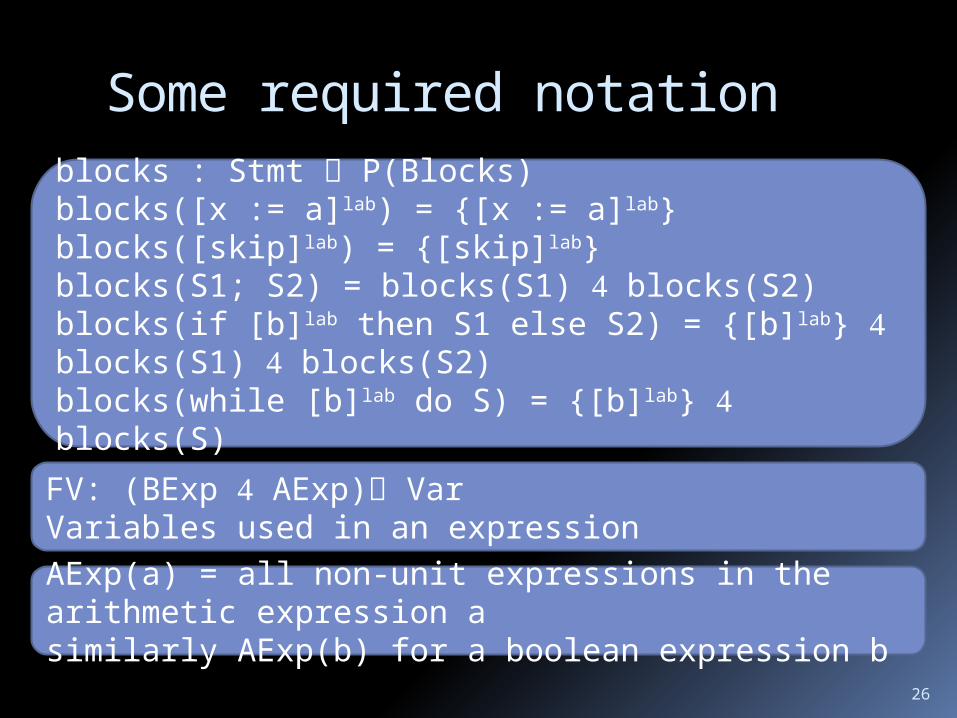
Some required notation
blocks : Stmt P(Blocks)blocks([x := a]lab) = {[x := a]lab}blocks([skip]lab) = {[skip]lab}blocks(S1; S2) = blocks(S1) blocks(S2)blocks(if [b]lab then S1 else S2) = {[b]lab} blocks(S1) blocks(S2)blocks(while [b]lab do S) = {[b]lab} blocks(S)
FV: (BExp AExp) Var Variables used in an expressionAExp(a) = all non-unit expressions in the arithmetic expression asimilarly AExp(b) for a boolean expression b

27
Available Expressions Analysis
For each program point, which expressions must have already been computed, and not later modified, on all paths to the program point
[x := a+b]1;[y := a*b]2;while [y > a+b]3 ( [a := a + 1]4; [x := a + b]5
)
(a+b) always available at label
3

28
Available Expressions Analysis Property space
inAE, outAE: Lab (AExp) Mapping a label to set of arithmetic
expressions available at that label
Dataflow equations Flow equations – how to join incoming
dataflow facts Effect equations - given an input set of
expressions S, what is the effect of a statement
29
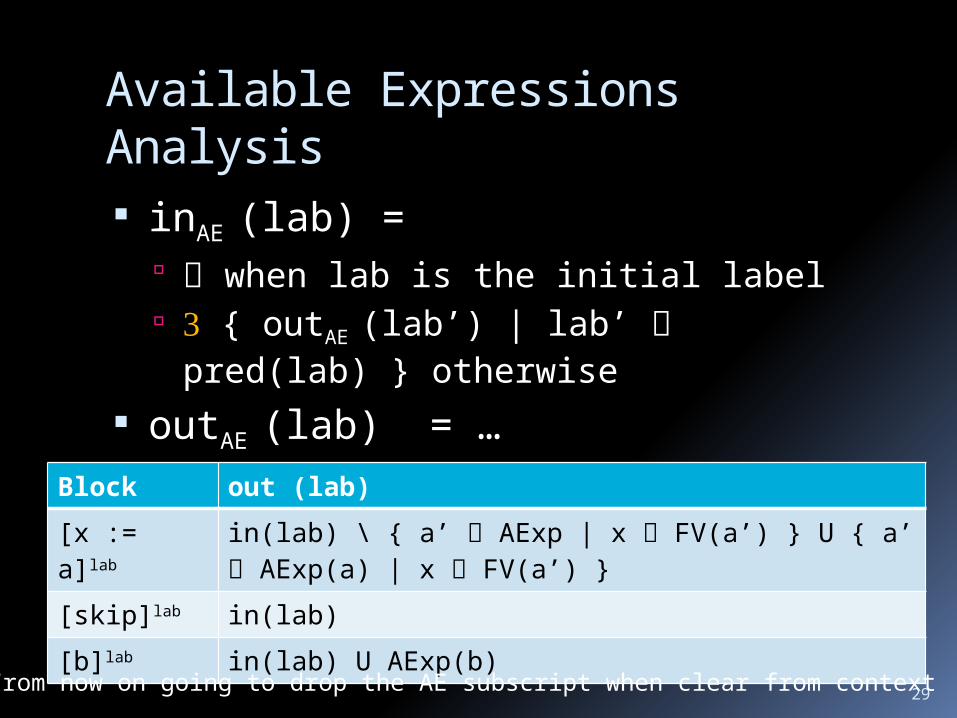
inAE (lab) = when lab is the initial label { outAE (lab’) | lab’ pred(lab) }
otherwise
outAE (lab) = …Block out (lab)
[x := a]lab in(lab) \ { a’ AExp | x FV(a’) } U { a’ AExp(a) | x FV(a’) }
[skip]lab in(lab)
[b]lab in(lab) U AExp(b)
Available Expressions Analysis
From now on going to drop the AE subscript when clear from context

30
Transfer Functions1: x = a+b
2: y:=a*b
3: y > a+b
4: a=a+1
5: x=a+b
out(1) = in(1) U { a+b }
out(2) = in(2) U { a*b }
in(1) = in(2) = out(1)in(3) = out(2) out(5)in(4) = out(3)in(5) = out(4)
out(4) = in(4) \ { a+b,a*b,a+1 }
out(5) = in(5) U { a+b }
out(3) = in(3) U { a+ b }
[x := a+b]1;[y := a*b]2;while [y > a+b]3 ( [a := a + 1]4; [x := a + b]5
)

31
Solution
1: x = a+b
2: y:=a*b
3: y > a+b
4: a=a+1
5: x=a+b
in(2) = out(1) = { a + b }
out(2) = { a+b, a*b }
out(4) =
out(5) = { a+b }
in(4) = out(3) = { a+ b }
in(1) =
in(3) = { a + b }
32
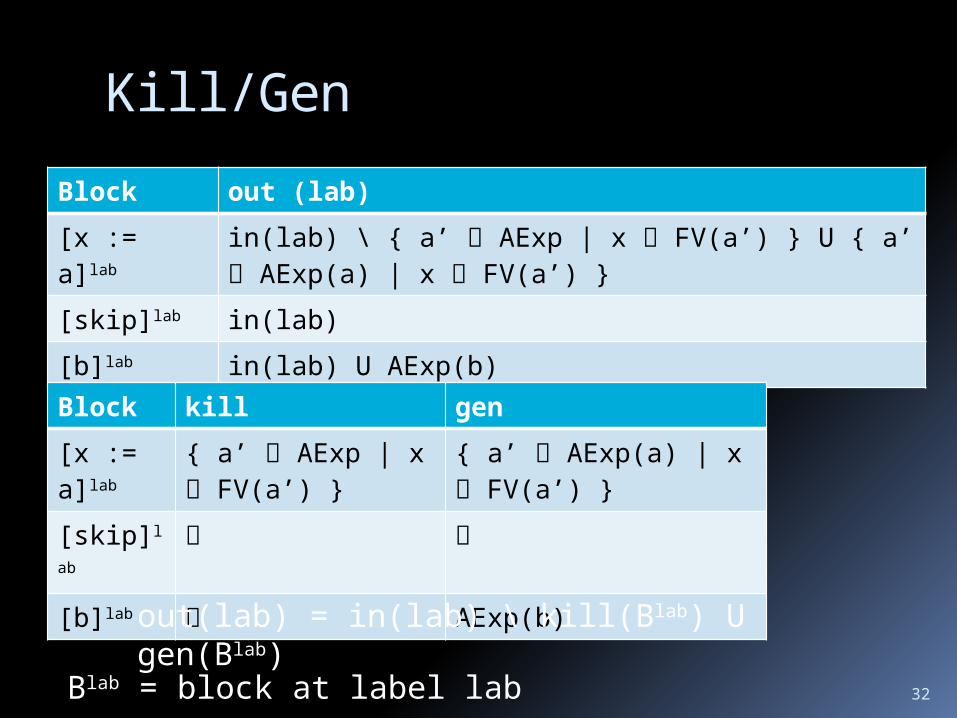
Kill/Gen
Block out (lab)
[x := a]lab in(lab) \ { a’ AExp | x FV(a’) } U { a’ AExp(a) | x FV(a’) }
[skip]lab in(lab)
[b]lab in(lab) U AExp(b)
Block kill gen
[x := a]lab
{ a’ AExp | x FV(a’) }
{ a’ AExp(a) | x FV(a’) }
[skip]lab
[b]lab AExp(b)
out(lab) = in(lab) \ kill(Blab) U gen(Blab)
Blab = block at label lab
33
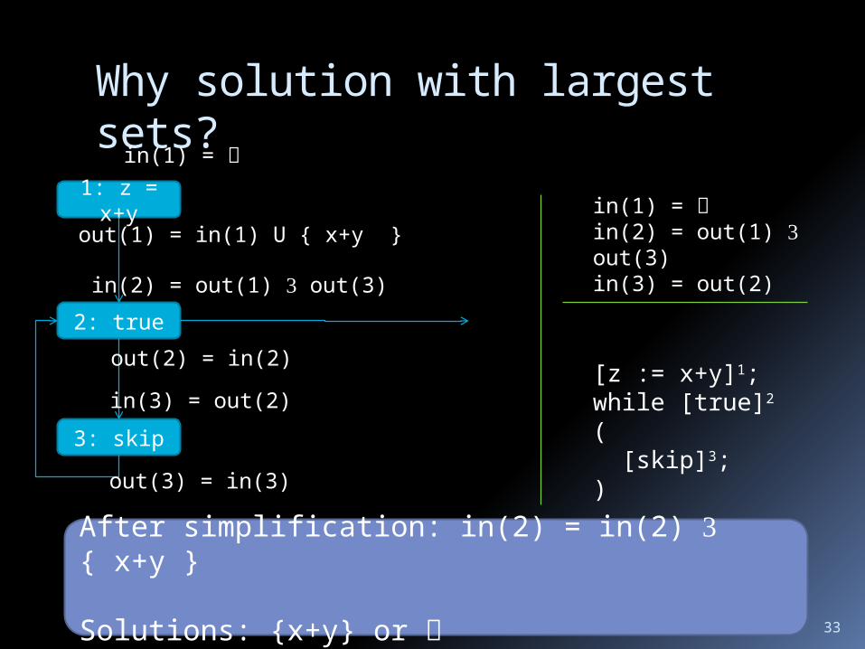
Why solution with largest sets?
1: z = x+y
2: true
3: skip
out(1) = in(1) U { x+y }in(1) = in(2) = out(1) out(3)in(3) = out(2)
out(3) = in(3)
out(2) = in(2)[z := x+y]1;while [true]2 ( [skip]3;)
in(1) =
After simplification: in(2) = in(2) { x+y }
Solutions: {x+y} or
in(2) = out(1) out(3)
in(3) = out(2)
34
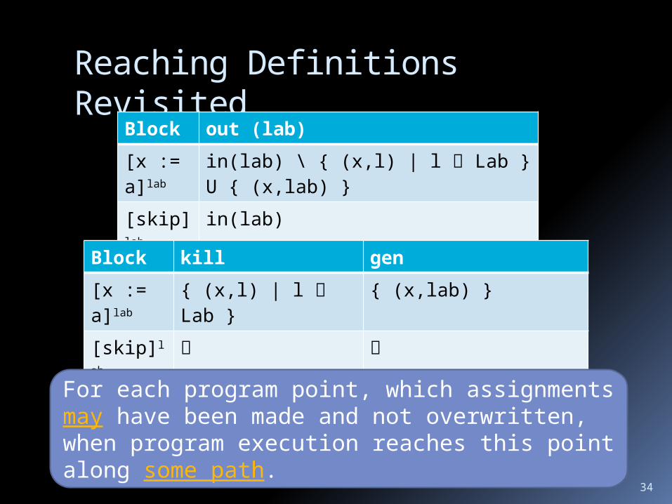
Reaching Definitions Revisited
Block out (lab)
[x := a]lab
in(lab) \ { (x,l) | l Lab } U { (x,lab) }
[skip]la
b
in(lab)
[b]lab in(lab) Block kill gen
[x := a]lab
{ (x,l) | l Lab } { (x,lab) }
[skip]lab
[b]lab
For each program point, which assignments may have been made and not overwritten, when program execution reaches this point along some path.

35
Why solution with smallest sets?
1: z = x+y
2: true
3: skip
out(1) = ( in(1) \ { (z,?) } ) U { (z,1) }in(1) = { (x,?),(y,?),(z,?) } in(2) = out(1) U out(3)in(3) = out(2)
out(3) = in(3)
out(2) = in(2)[z := x+y]1;while [true]2 ( [skip]3;)
in(1) = { (x,?),(y,?),(z,?) }
After simplification: in(2) = in(2) U { (x,?),(y,?),(z,1) }
Many solutions: any superset of { (x,?),(y,?),(z,1) }
in(2) = out(1) U out(3)
in(3) = out(2)

36
Live Variables
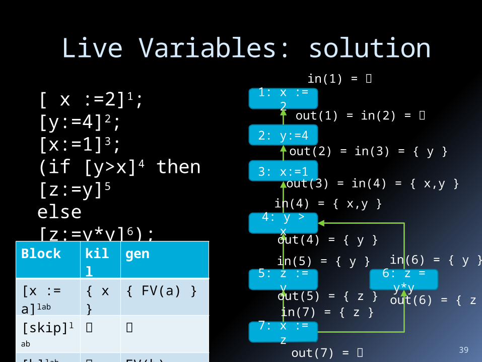
For each program point, which variables may be live at the exit from the point.
[ x :=2]1; [y:=4]2; [x:=1]3; (if [y>x]4 then [z:=y]5 else [z:=y*y]6); [x:=z]7
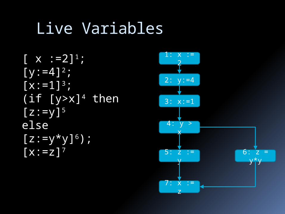
[ x :=2]1; [y:=4]2; [x:=1]3; (if [y>x]4 then [z:=y]5 else [z:=y*y]6); [x:=z]7
Live Variables
1: x := 2
2: y:=4
4: y > x
5: z := y
7: x := z
6: z = y*y
3: x:=1
38
1: x := 2
2: y:=4
4: y > x
5: z := y
7: x := z
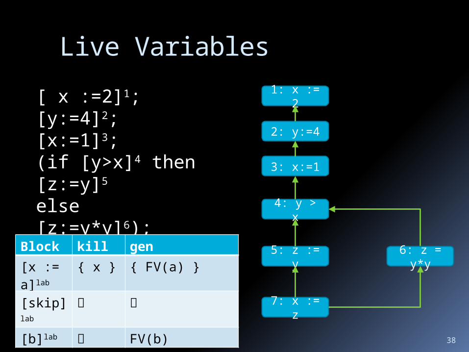
[ x :=2]1; [y:=4]2; [x:=1]3; (if [y>x]4 then [z:=y]5 else [z:=y*y]6); [x:=z]7
6: z = y*y
Live Variables
Block kill gen
[x := a]lab
{ x } { FV(a) }
[skip]la
b
[b]lab FV(b)
3: x:=1
39
1: x := 2
2: y:=4
4: y > x
5: z := y
7: x := z
[ x :=2]1; [y:=4]2; [x:=1]3; (if [y>x]4 then [z:=y]5 else [z:=y*y]6); [x:=z]7
6: z = y*y
Live Variables: solution
Block kill gen
[x := a]lab
{ x }
{ FV(a) }
[skip]lab
[b]lab FV(b)
3: x:=1
in(1) =
out(1) = in(2) =
out(2) = in(3) = { y }
out(3) = in(4) = { x,y }
in(7) = { z }
out(7) =
out(6) = { z }
in(6) = { y }
out(5) = { z }
in(5) = { y }
in(4) = { x,y }
out(4) = { y }
40
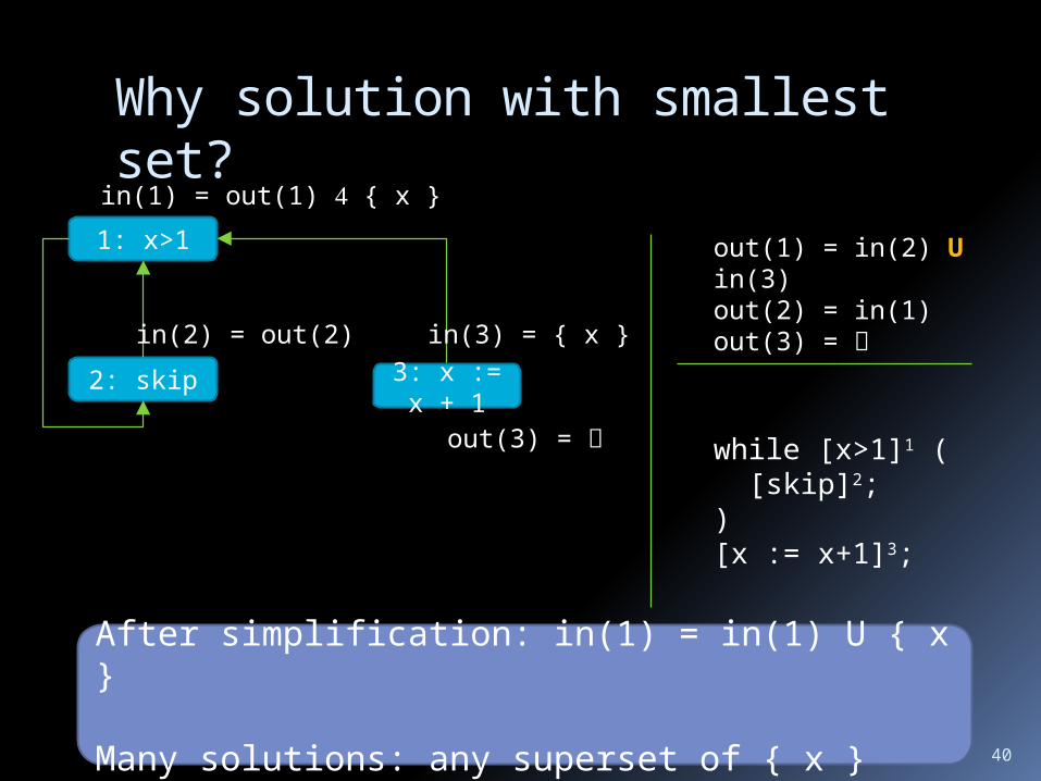
Why solution with smallest set?
1: x>1
2: skip
out(1) = in(2) U in(3)out(2) = in(1)out(3) =
out(3) =
in(2) = out(2)
while [x>1]1 ( [skip]2;)[x := x+1]3;
After simplification: in(1) = in(1) U { x }
Many solutions: any superset of { x }
3: x := x + 1
in(3) = { x }
in(1) = out(1) { x }
41
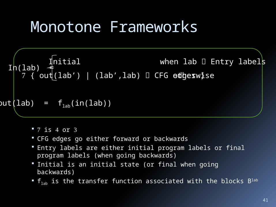
Monotone Frameworks
is or CFG edges go either forward or backwards Entry labels are either initial program labels or final
program labels (when going backwards) Initial is an initial state (or final when going backwards) flab is the transfer function associated with the blocks Blab
In(lab) = { out(lab’) | (lab’,lab) CFG edges }
Initial when lab Entry labels
otherwise
out(lab) = flab(in(lab))
42
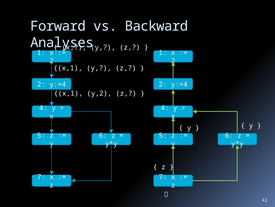
Forward vs. Backward Analyses
1: x := 2
2: y:=4
4: y > x
5: z := y
7: x := z
6: z = y*y
1: x := 2
2: y:=4
4: y > x
5: z := y
7: x := z
6: z = y*y
{(x,1), (y,?), (z,?) }
{ (x,?), (y,?), (z,?) }
{(x,1), (y,2), (z,?) }
{ z }
{ y }{ y }
43
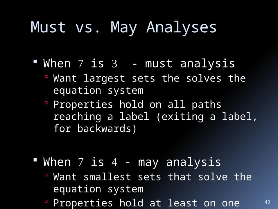
Must vs. May Analyses
When is - must analysis Want largest sets the solves the
equation system Properties hold on all paths reaching a
label (exiting a label, for backwards)
When is - may analysis Want smallest sets that solve the
equation system Properties hold at least on one path
reaching a label (existing a label, for backwards)
44
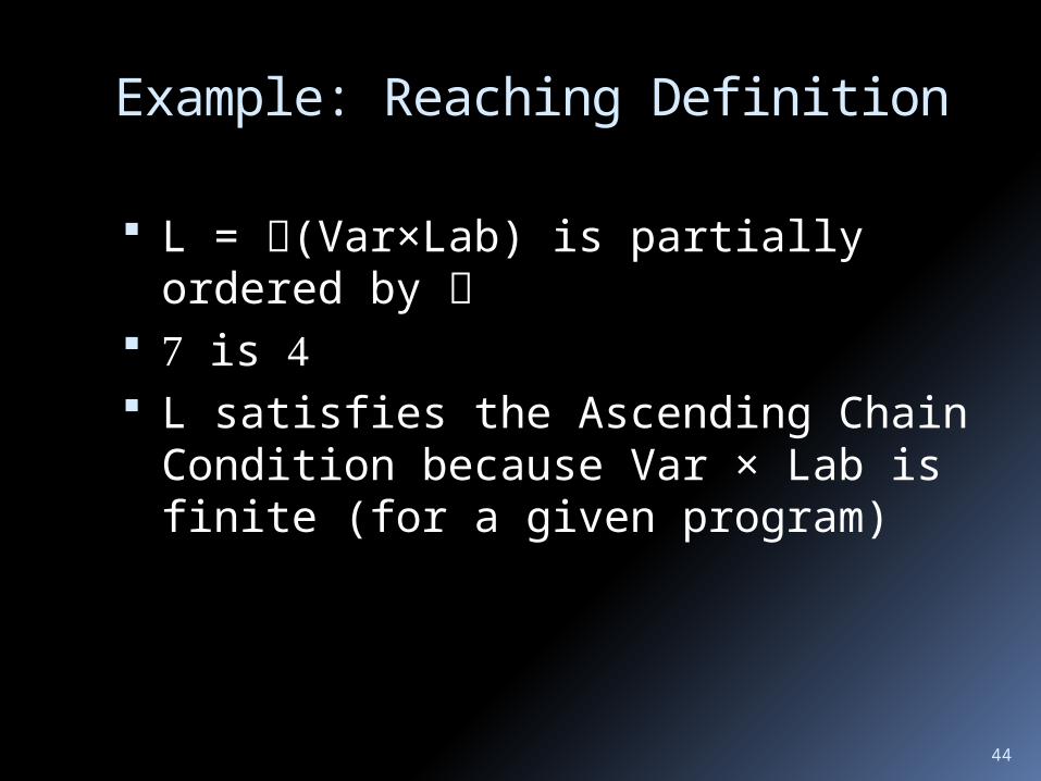
Example: Reaching Definition
L = (Var×Lab) is partially ordered by
is L satisfies the Ascending Chain
Condition because Var × Lab is finite (for a given program)
45
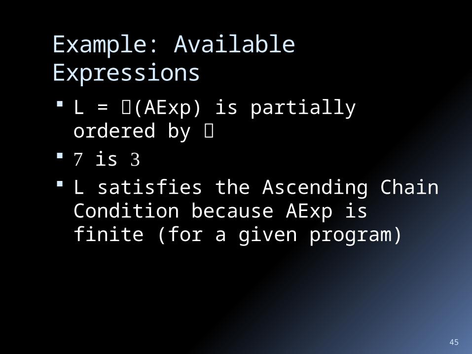
Example: Available Expressions L = (AExp) is partially ordered by is L satisfies the Ascending Chain
Condition because AExp is finite (for a given program)

46
Analyses Summary
Reaching Definitions
Available Expressions
Live Variables
L (Var x Lab) (AExp) (Var)
AExp
Initial { (x,?) | x Var}
Entry labels { init } { init } final
Direction Forward Forward Backward
F { f: L L | k,g : f(val) = (val \ k) U g }
flab flab(val) = (val \ kill) gen
47
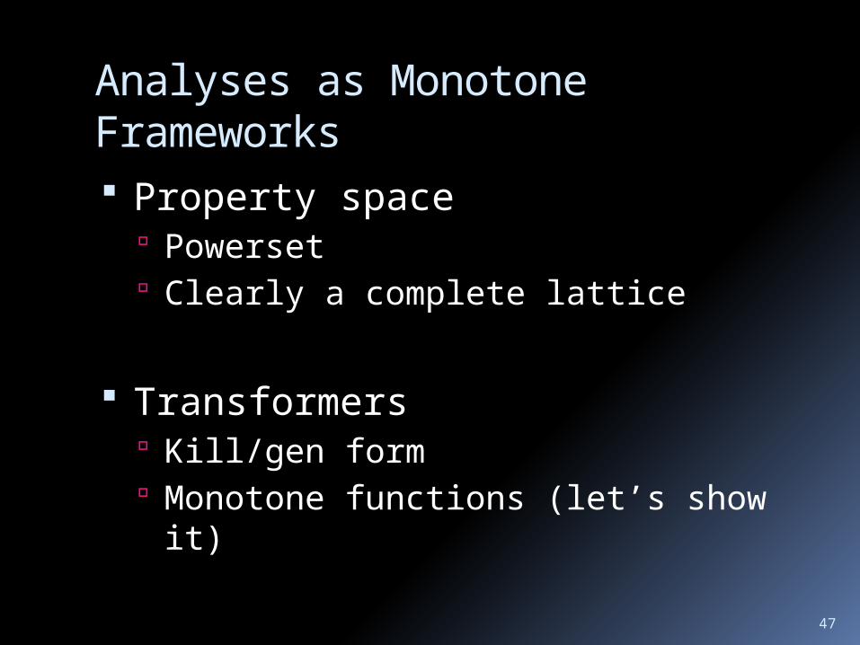
Analyses as Monotone Frameworks Property space
Powerset Clearly a complete lattice
Transformers Kill/gen form Monotone functions (let’s show it)
48
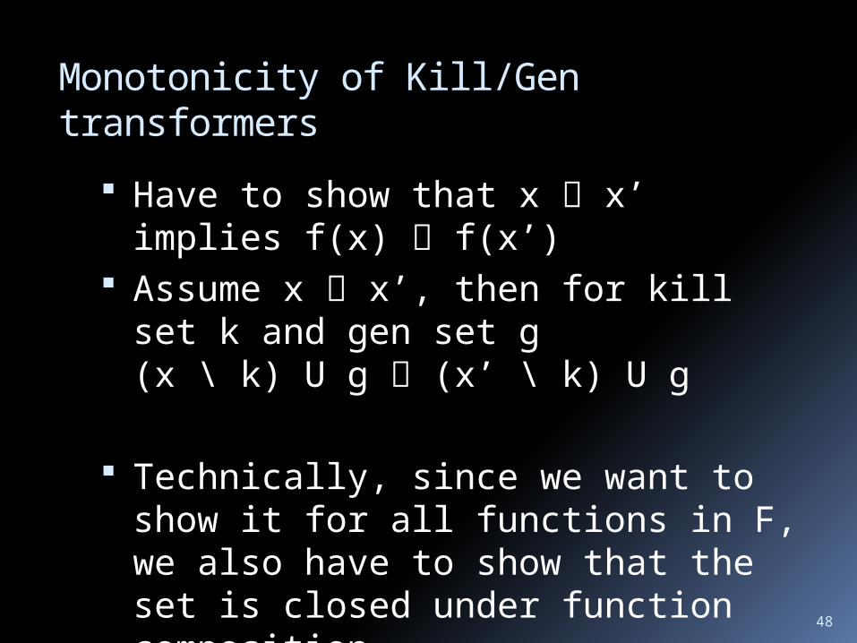
Monotonicity of Kill/Gen transformers
Have to show that x x’ implies f(x) f(x’)
Assume x x’, then for kill set k and gen set g(x \ k) U g (x’ \ k) U g
Technically, since we want to show it for all functions in F, we also have to show that the set is closed under function composition
49
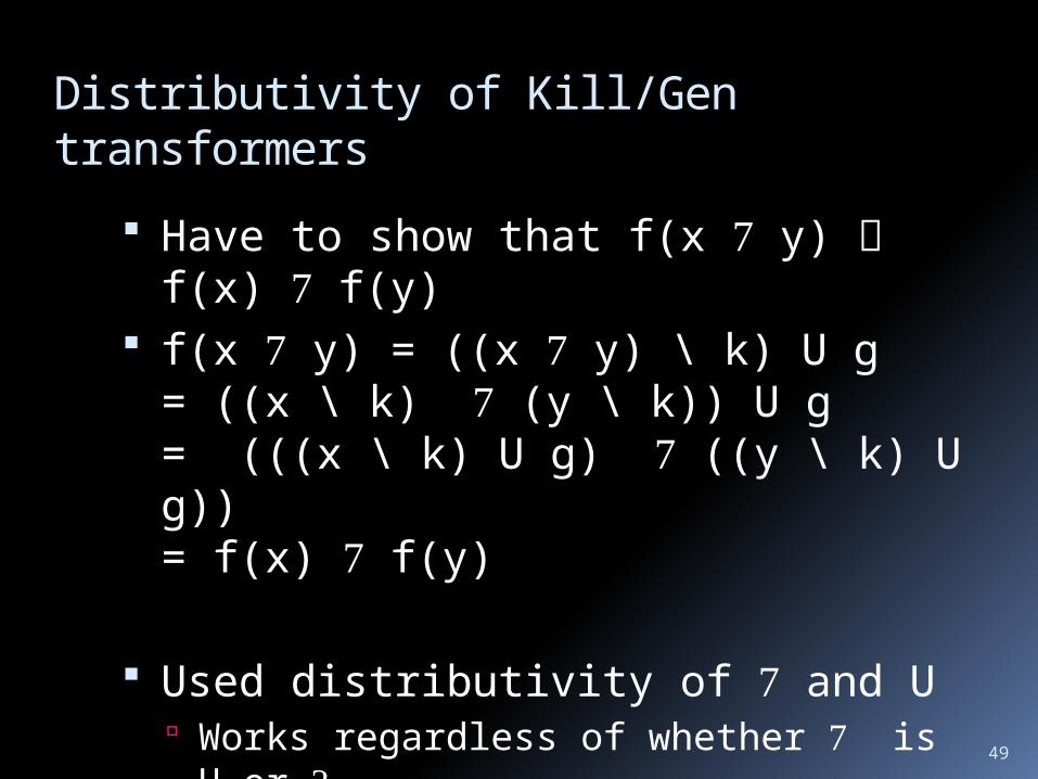
Distributivity of Kill/Gen transformers
Have to show that f(x y) f(x) f(y) f(x y) = ((x y) \ k) U g
= ((x \ k) (y \ k)) U g= (((x \ k) U g) ((y \ k) U g))= f(x) f(y)
Used distributivity of and U Works regardless of whether is U or