Lecture 13 - University of Waterloovganesh/TEACHING/S2014... · by Prof. Vijay Ganesh) Lecture 13 27 Notes • Main has no argument or local variables and its result is never used;

Prof. Alex Aiken Original Slides (Modified by Prof. Vijay Ganesh) Lecture 13

1

Run-time Environments

Lecture 13


2

What have we covered so far?

•  We have covered the front-end phases –  Lexical analysis (Lexer, regular expressions,...) –  Parsing (CFG, Top-down, bottom-up,…) –  Semantic analysis (Type systems, semantic actions)

•  Next are the back-end phases

–  Optimization –  Code generation

•  We’ll do code generation first . . .


3

Run-time environments

•  Before discussing code generation, we need to understand what we are trying to generate

•  There are a number of standard techniques for structuring executable code that are widely used


4

Outline

•  Management of run-time resources

•  Correspondence between –  static (compile-time) and –  dynamic (run-time) structures

•  Storage organization


5

Run-time Resources

•  Execution of a program is initially under the control of the operating system

•  When a program is invoked: –  The OS allocates space for the program –  The code is loaded into part of the space –  The OS “jumps to” the entry point (i.e., “main”)


6

Memory Layout

Low Address

High Address

Memory

Code

Other Space


7

Notes

•  By tradition, pictures of machine organization have: –  Low address at the top –  High address at the bottom –  Lines delimiting areas for different kinds of data

•  These pictures are simplifications –  E.g., not all memory need be contiguous


8

What is Other Space?

•  Holds all data for the program •  Other Space = Data Space

•  Compiler is responsible for: –  Generating code –  Orchestrating use of the data area


9

Code Generation Goals

•  Two goals: –  Correctness –  Speed

•  Most complications in code generation come from trying to be fast as well as correct


10

Assumptions about Execution

1.  Execution is sequential; control moves from one point in a program to another in a well-defined order

2.  When a procedure is called, control eventually returns to the point immediately after the call

Do these assumptions always hold?


11

Activations

•  An invocation of procedure P is an activation of P

•  The lifetime of an activation of P is –  All the steps to execute P –  Including all the steps in procedures P calls


12

Lifetimes of Variables

•  The lifetime of a variable x is the portion of execution in which x is defined

•  Note that –  Lifetime is a dynamic (run-time) concept –  Scope is a static concept


13

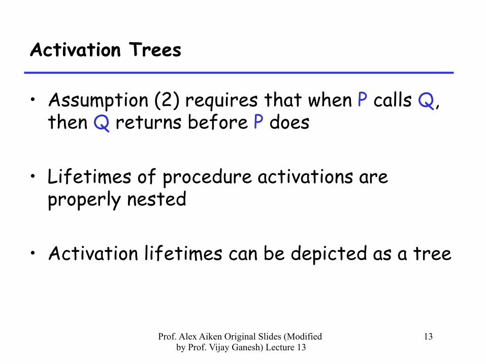
Activation Trees

•  Assumption (2) requires that when P calls Q, then Q returns before P does

•  Lifetimes of procedure activations are properly nested

•  Activation lifetimes can be depicted as a tree


14

Example 1

Class Main { g() : Int { 1 }; f(): Int { g() }; main(): Int {{ g(); f(); }};

} Main

f g

g


15

Example 2

Class Main { g() : Int { 1 }; f(x:Int): Int { if x = 0 then g() else f(x - 1) fi}; main(): Int {{f(3); }};

} What is the activation tree for this example?


16

Notes

•  The activation tree depends on run-time behavior

•  The activation tree may be different for every program input

•  Since activations are properly nested, a stack can track concurrently active procedures


17

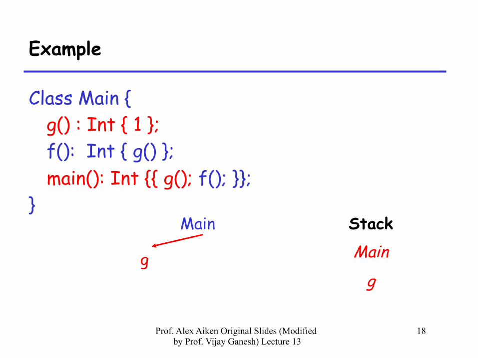
Example


} Main Stack

Main


18

Example


} Main

g

Stack

Main

g


19

Example


} Main

g f

Stack

Main

f


20

Example


} Main

f g

g

Stack

Main

f g


21

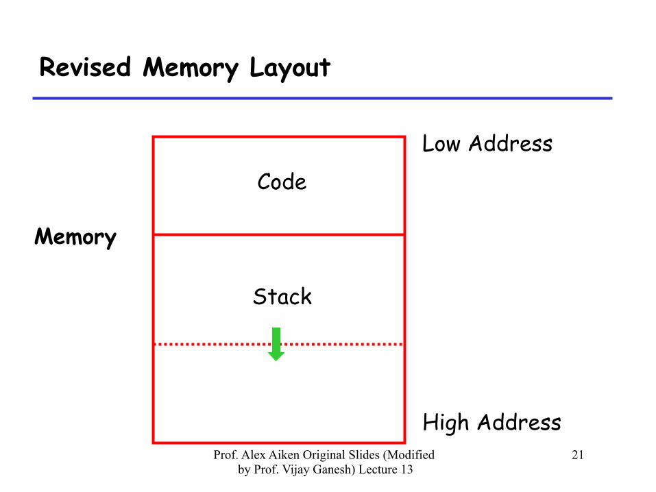
Revised Memory Layout

Low Address

High Address

Memory

Code

Stack


22

Activation Records

•  The information needed to manage one procedure activation is called an activation record (AR) or frame

•  If procedure F calls G, then G’s activation record contains a mix of info about F and G.


23

What is in G’s AR when F calls G?

•  F is “suspended” until G completes, at which point F resumes. G’s AR contains information needed to resume execution of F.

•  G’s AR may also contain: –  G’s return value (needed by F) –  Actual parameters to G (supplied by F) –  Space for G’s local variables


24

The Contents of a Typical AR for G

•  Space for G’s return value •  Actual parameters •  Pointer to the previous activation record

–  The control link; points to AR of caller of G •  Machine status prior to calling G

–  Contents of registers & program counter –  Local variables

•  Other temporary values


25

Example 2, Revisited

Class Main { g() : Int { 1 }; f(x:Int):Int {if x=0 then g() else f(x - 1)(**)fi}; main(): Int {{f(3); (*)

}};} AR for f:

result argument control link return address


26

Stack After Two Calls to f

Main

(**)

2 (result) f (*)

3 (result) f


27

Notes

•  Main has no argument or local variables and its result is never used; its AR is uninteresting

•  (*) and (**) are return addresses of the invocations of f –  The return address is where execution resumes

after a procedure call finishes

•  This is only one of many possible AR designs –  Would also work for C, Pascal, FORTRAN, etc.


28

The Main Point

The compiler must determine, at compile-time,

the layout of activation records and generate code that correctly accesses locations in the

activation record

Thus, the AR layout and the code generator must be designed together!


29

Example

The picture shows the state after the call to the 2nd invocation of f returns

Main

(**)

2 1 f (*)

3 (result) f


30

Discussion

•  The advantage of placing the return value 1st in a frame is that the caller can find it at a fixed offset from its own frame

•  There is nothing magic about this organization –  Can rearrange order of frame elements –  Can divide caller/callee responsibilities differently –  An organization is better if it improves execution

speed or simplifies code generation


31

Discussion (Cont.)

•  Real compilers hold as much of the frame as possible in registers –  Especially the method result and arguments


32

Globals

•  All references to a global variable point to the same object –  Can’t store a global in an activation record

•  Globals are assigned a fixed address once –  Variables with fixed address are “statically

allocated” •  Depending on the language, there may be

other statically allocated values


33

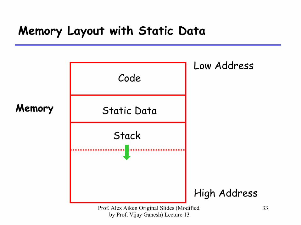
Memory Layout with Static Data

Low Address

High Address

Memory

Code

Stack

Static Data


34

Heap Storage

•  A value that outlives the procedure that creates it cannot be kept in the AR

method foo() { new Bar } The Bar value must survive deallocation of foo’s AR

•  Languages with dynamically allocated data use a heap to store dynamic data


35

Notes

•  The code area contains object code –  For most languages, fixed size and read only

•  The static area contains data (not code) with fixed addresses (e.g., global data) –  Fixed size, may be readable or writable

•  The stack contains an AR for each currently active procedure –  Each AR usually fixed size, contains locals

•  Heap contains all other data –  In C, heap is managed by malloc and free


36

Notes (Cont.)

•  Both the heap and the stack grow

•  Must take care that they don’t grow into each other

•  Solution: start heap and stack at opposite ends of memory and let them grow towards each other


37

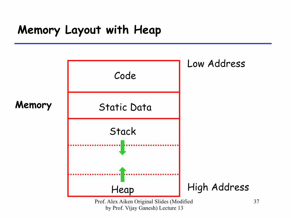
Memory Layout with Heap

Low Address

High Address

Memory

Code

Stack

Static Data

Heap


38

Data Layout

•  Low-level details of machine architecture are important in laying out data for correct code and maximum performance

•  Chief among these concerns is alignment


39

Alignment

•  Most modern machines are (still) 32 bit –  8 bits in a byte –  4 bytes in a word –  Machines are either byte or word addressable

•  Data is word aligned if it begins at a word boundary

•  Most machines have some alignment restrictions –  Or performance penalties for poor alignment


40

Alignment (Cont.)

•  Example: A string “Hello”

Takes 5 characters (without a terminating \0)

•  To word align next datum, add 3 “padding” characters to the string

•  The padding is not part of the string, it’s just unused memory


41

Next Topic: Stack Machines

•  A simple evaluation model •  No variables or registers •  A stack of values for intermediate results •  Each instruction:

–  Takes its operands from the top of the stack –  Removes those operands from the stack –  Computes the required operation on them –  Pushes the result on the stack


42

Example of Stack Machine Operation

•  The addition operation on a stack machine

5 7 9 …

5

7

9 …

pop

⊕

add

12 9 …

push


43

Example of a Stack Machine Program

•  Consider two instructions –  push i - place the integer i on top of the stack –  add - pop two elements, add them and put the result back on the stack

•  A program to compute 7 + 5: push 7 push 5 add


44

Why Use a Stack Machine ?

•  Each operation takes operands from the same place and puts results in the same place

•  This means a uniform compilation scheme

•  And therefore a simpler compiler


45

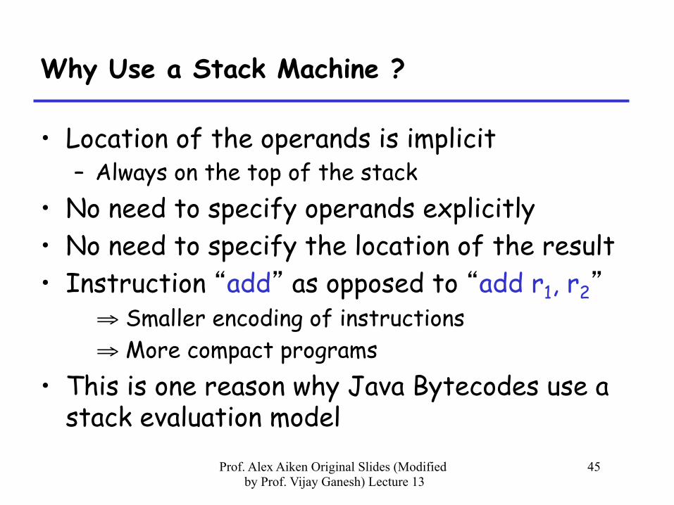
Why Use a Stack Machine ?

•  Location of the operands is implicit –  Always on the top of the stack

•  No need to specify operands explicitly •  No need to specify the location of the result •  Instruction “add” as opposed to “add r1, r2”

⇒ Smaller encoding of instructions ⇒ More compact programs

•  This is one reason why Java Bytecodes use a stack evaluation model


46

Optimizing the Stack Machine

•  The add instruction does 3 memory operations –  Two reads and one write to the stack –  The top of the stack is frequently accessed

•  Idea: keep the top of the stack in a register (called accumulator) –  Register accesses are faster

•  The “add” instruction is now acc ← acc + top_of_stack –  Only one memory operation!


47

Stack Machine with Accumulator

Invariants •  The result of an expression is in the

accumulator

•  For op(e1,…,en) push the accumulator on the stack after computing e1,…,en-1 –  After the operation pops n-1 values

•  Expression evaluation preserves the stack


48

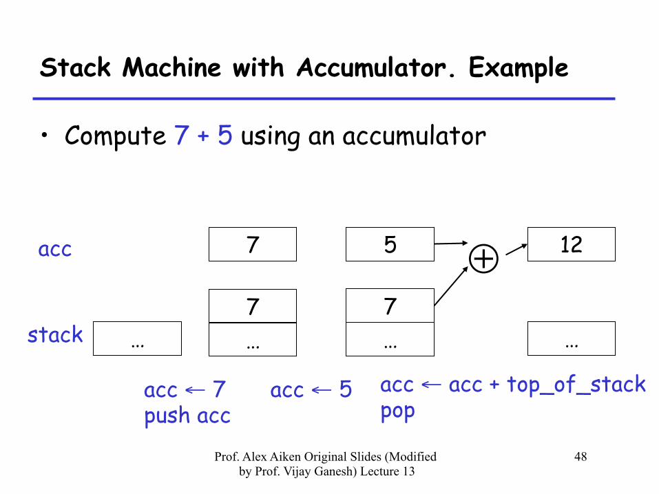
Stack Machine with Accumulator. Example

•  Compute 7 + 5 using an accumulator

…

acc

stack

5

7 …

acc ← 5

12

…

⊕

acc ← acc + top_of_stack pop

…

7

acc ← 7 push acc

7


49

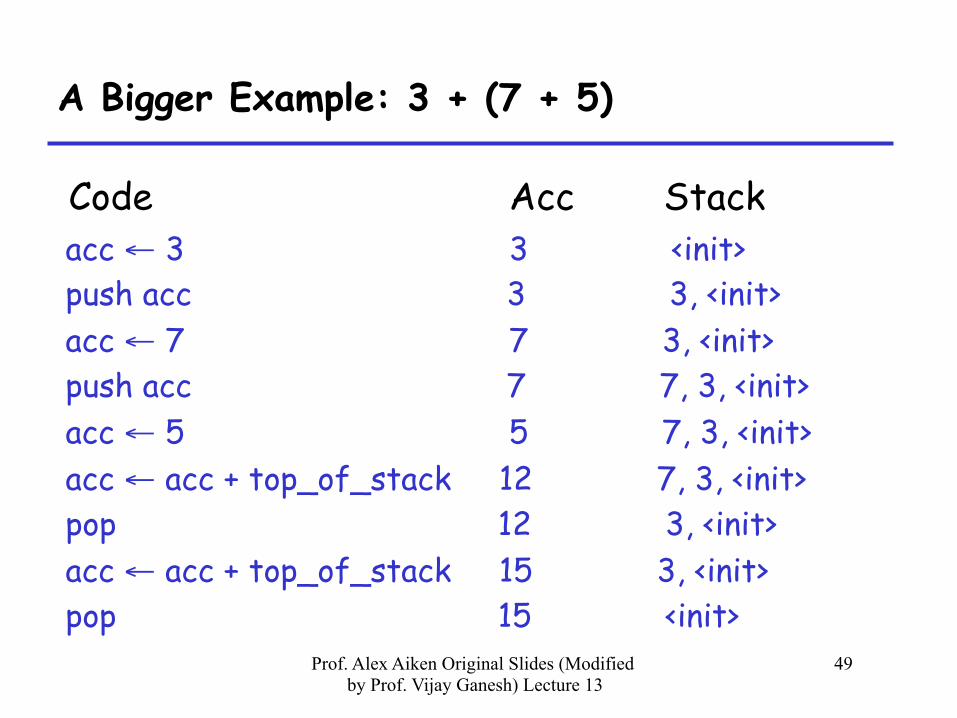
A Bigger Example: 3 + (7 + 5)

Code Acc Stack acc ← 3 3 <init> push acc 3 3, <init> acc ← 7 7 3, <init> push acc 7 7, 3, <init> acc ← 5 5 7, 3, <init> acc ← acc + top_of_stack 12 7, 3, <init> pop 12 3, <init> acc ← acc + top_of_stack 15 3, <init> pop 15 <init>


50

Notes

•  It is very important evaluation of a subexpression preserves the stack –  Stack before the evaluation of 7 + 5 is 3, <init> –  Stack after the evaluation of 7 + 5 is 3, <init> –  The first operand is on top of the stack

Documents

Lecture 13 - University of Waterloovganesh/TEACHING/S2014... · by Prof. Vijay Ganesh) Lecture 13 27 Notes • Main has no argument or local variables and its result is never used;