1

Lecture 13: Stability and Control I

We are learning how to analyze mechanismsbut what we’d like to do is make them do our bidding

We want to be able to control them —to make a robot trace a particular path, say

A full study of this is well beyond the scope of this coursewe’ll just do enough to give you the flavor of the thing

and to let you do some things

2

You might think that if we knew the forces/torques to hold a robot somewherethat we could just set them to those values and we’d be home free

Not true, and the key lies in stability

We want to have a system that is close to where it should bewhen the forces are close to where they should be

Eventually we can design transient forces that will control our systems

3

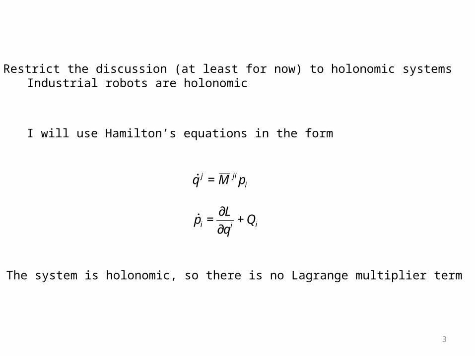
Restrict the discussion (at least for now) to holonomic systemsIndustrial robots are holonomic

I will use Hamilton’s equations in the form

€

˙ p i =∂L

∂qi+ Qi

€

˙ q j = M ji pi

The system is holonomic, so there is no Lagrange multiplier term

4

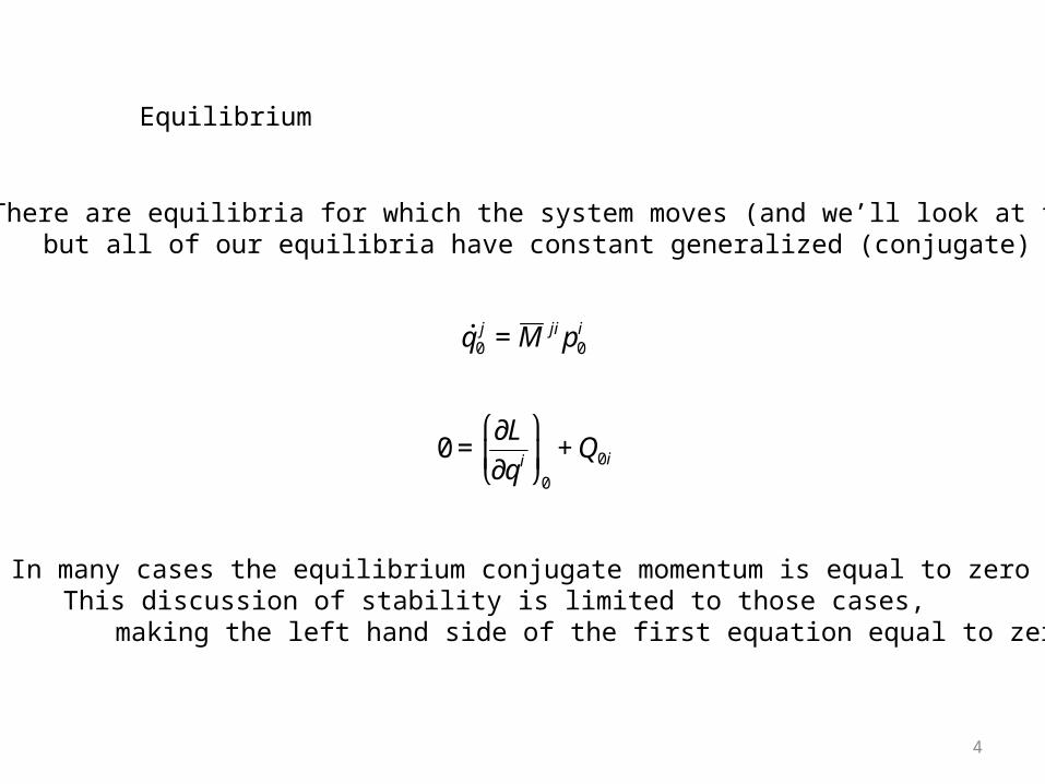
Equilibrium

There are equilibria for which the system moves (and we’ll look at those)but all of our equilibria have constant generalized (conjugate) momenta

€

0 =∂L

∂qi

⎛

⎝ ⎜

⎞

⎠ ⎟0

+ Q0i€

˙ q 0j = M ji p0

i

In many cases the equilibrium conjugate momentum is equal to zeroThis discussion of stability is limited to those cases,

making the left hand side of the first equation equal to zero

5

It is generally possible to solve the equilibrium equations for the equilibrium (generalized) forces

I’ll do this eventually using a robot example

Let’s suppose we’ve done that

The big question is:

What happens if we don’t get the forces exactly right?

Will the position of the robot, say, be close to what we wantor will it be completely different?

6

In other wordsIs the robot stable or unstable?

I need some vocabulary (all for linear stability)

I’m talking about small errors, which I can address using linear stability

Nonlinear stability is beyond the scope of the course

stable: if we move the system away from equilibrium, the system will go back

unstable: if we move the system away from equilibrium, the error will grow (initially) exponentially

marginally stable: if we move the system away from equilibrium, the error will oscillate about its reference position

7

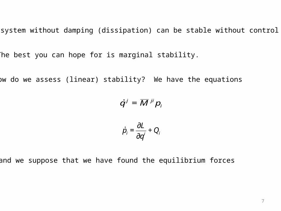
No system without damping (dissipation) can be stable without control

The best you can hope for is marginal stability.

How do we assess (linear) stability? We have the equations

€

˙ p i =∂L

∂qi+ Qi€

˙ q j = M ji pi

and we suppose that we have found the equilibrium forces

8

€

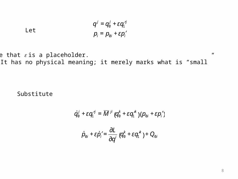
q j = q0j + ε ′ q 1

j

pi = p0i + ε ′ p i

Note that e is a placeholder. It has no physical meaning; it merely marks what is “small”

Let

€

˙ p 0i + ε ′ ˙ p i =∂L

∂qiq0

k + ε ′ q 1k

( ) + Q0i

€

˙ q 0j + ε ′ q 1

j = M ji q0k + ε ′ q 1

k( ) p0i + ε ′ p i( )

Substitute

9

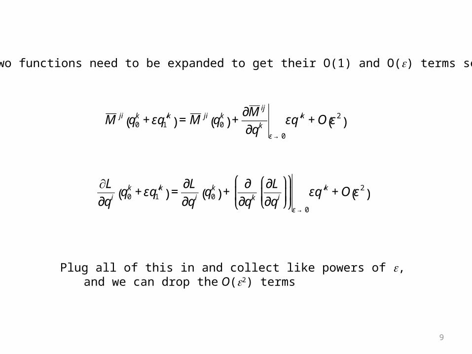
The two functions need to be expanded to get their O(1) and O(e) terms separated

€

M ji q0k + ε ′ q 1

k( ) = M ji q0

k( ) +

∂M ij

∂qk

ε →0

ε ′ q k + O ε 2( )

€

∂L

∂qiq0

k + ε ′ q 1k

( ) =∂L

∂qiq0

k( ) +

∂

∂qk

∂L

∂qi

⎛

⎝ ⎜

⎞

⎠ ⎟

⎛

⎝ ⎜

⎞

⎠ ⎟ε →0

ε ′ q k + O ε 2( )

Plug all of this in and collect like powers of e, and we can drop the O(e2) terms

10

€

˙ q 0j + ε ′ q 1

j = M ji q0k

( ) +∂M ij

∂qk

ε →0

ε ′ q k ⎛

⎝ ⎜

⎞

⎠ ⎟ p0i + ε ′ p i( )

€

˙ q 0j + ε ′ q 1

j = M ji q0k

( ) p0i + ε ′ p i( ) +∂M ij

∂qk

ε →0

ε ′ q k p0i

€

˙ q 0j = M ji q0

k( ) p0i

ε ′ q 1j = M ji q0

k( )ε ′ p i +

∂M ij

∂qk

ε →0

ε ′ q k p0i

€

′ q 1j = M ji q0

k( ) ′ p i +

∂M ij

∂qk

ε →0

′ q k p0i

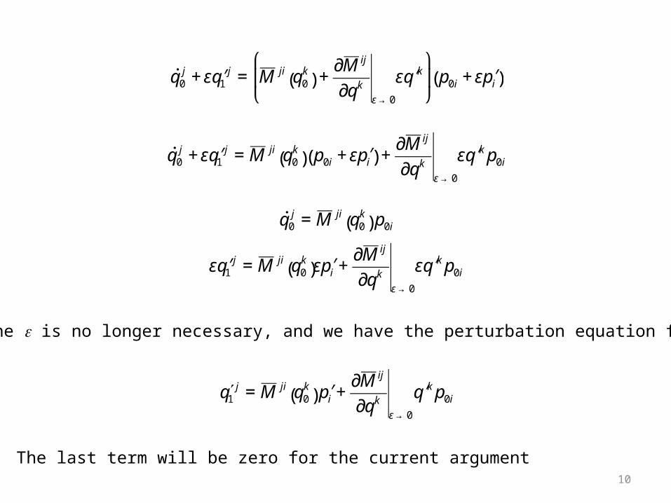
The e is no longer necessary, and we have the perturbation equation for q’

The last term will be zero for the current argument

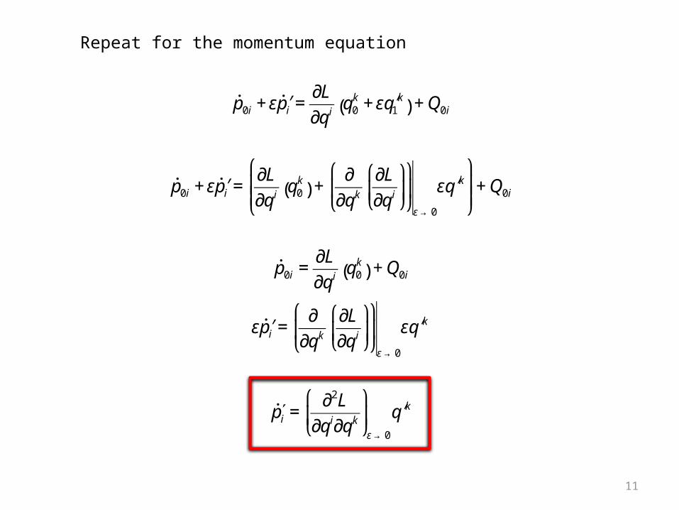
11

€

˙ p 0i + ε ′ ˙ p i =∂L

∂qiq0

k + ε ′ q 1k

( ) + Q0i

Repeat for the momentum equation

€

˙ p 0i + ε ′ ˙ p i =∂L

∂qiq0

k( ) +

∂

∂qk

∂L

∂qi

⎛

⎝ ⎜

⎞

⎠ ⎟

⎛

⎝ ⎜

⎞

⎠ ⎟ε →0

ε ′ q k ⎛

⎝ ⎜ ⎜

⎞

⎠ ⎟ ⎟+ Q0i

€

˙ p 0i =∂L

∂qiq0

k( ) + Q0i

ε ′ ˙ p i =∂

∂qk

∂L

∂qi

⎛

⎝ ⎜

⎞

⎠ ⎟

⎛

⎝ ⎜

⎞

⎠ ⎟ε →0

ε ′ q k

€

′ ˙ p i =∂2L

∂qi∂qk

⎛

⎝ ⎜

⎞

⎠ ⎟

ε →0

′ q k

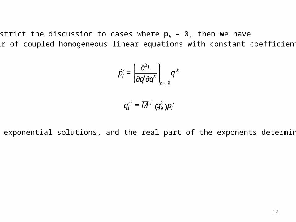
12

If we restrict the discussion to cases where p0 = 0, then we have a pair of coupled homogeneous linear equations with constant coefficients

€

′ q 1j = M ji q0

k( ) ′ p i

€

′ ˙ p i =∂2L

∂qi∂qk

⎛

⎝ ⎜

⎞

⎠ ⎟

ε →0

′ q k

These admit exponential solutions, and the real part of the exponents determine stability

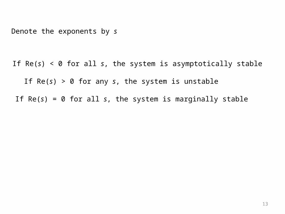
13

Denote the exponents by s

If Re(s) < 0 for all s, the system is asymptotically stable

If Re(s) > 0 for any s, the system is unstable

If Re(s) = 0 for all s, the system is marginally stable

14

??

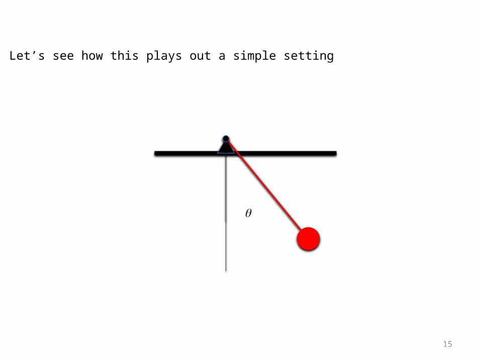
15

Let’s see how this plays out a simple setting

q

16

€

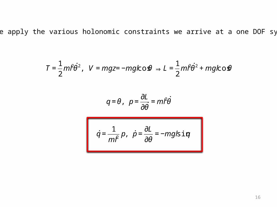
T =1

2ml2 ˙ θ 2, V = mgz = −mglcosθ ⇒ L =

1

2ml2 ˙ θ 2 + mglcosθ

If we apply the various holonomic constraints we arrive at a one DOF system

€

q = θ, p =∂L

∂ ˙ θ = ml2 ˙ θ

€

˙ q =1

ml2p, ˙ p =

∂L

∂θ= −mglsinq

17

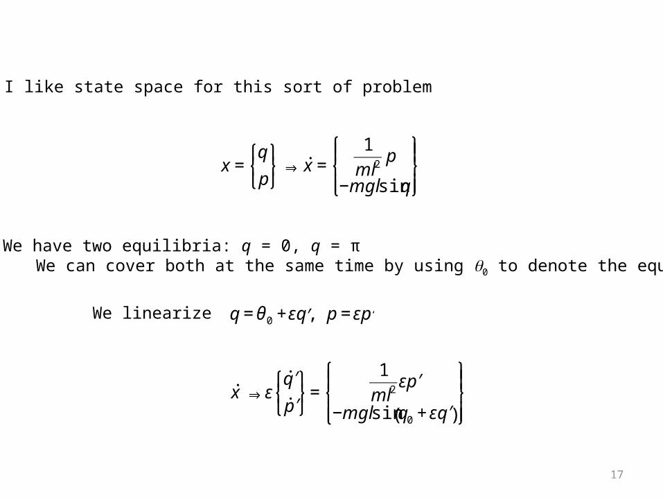
I like state space for this sort of problem

€

x =q

p

⎧ ⎨ ⎩

⎫ ⎬ ⎭⇒ ˙ x =

1

ml2p

−mglsinq

⎧ ⎨ ⎪

⎩ ⎪

⎫ ⎬ ⎪

⎭ ⎪

We have two equilibria: q = 0, q = πWe can cover both at the same time by using q0 to denote the equilibrium

€

˙ x ⇒ ε˙ ′ q

˙ ′ p

⎧ ⎨ ⎩

⎫ ⎬ ⎭=

1

ml2ε ′ p

−mglsin q0 + ε ′ q ( )

⎧ ⎨ ⎪

⎩ ⎪

⎫ ⎬ ⎪

⎭ ⎪

We linearize

€

q = θ 0 +ε ′ q , p = ε ′ p

18

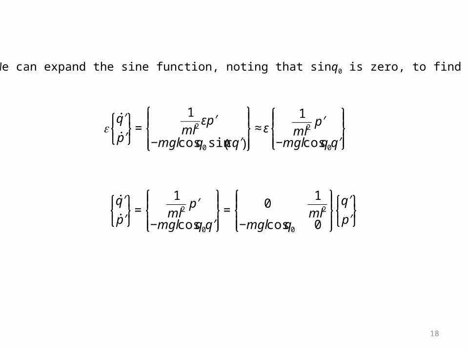
We can expand the sine function, noting that sinq0 is zero, to find

€

ε˙ ′ q

˙ ′ p

⎧ ⎨ ⎩

⎫ ⎬ ⎭=

1

ml2ε ′ p

−mglcosq0 sin ε ′ q ( )

⎧ ⎨ ⎪

⎩ ⎪

⎫ ⎬ ⎪

⎭ ⎪≈ ε

1

ml2′ p

−mglcosq0 ′ q

⎧ ⎨ ⎪

⎩ ⎪

⎫ ⎬ ⎪

⎭ ⎪

€

˙ ′ q

˙ ′ p

⎧ ⎨ ⎩

⎫ ⎬ ⎭=

1

ml2′ p

−mglcosq0 ′ q

⎧ ⎨ ⎪

⎩ ⎪

⎫ ⎬ ⎪

⎭ ⎪= 0

1

ml2

−mglcosq0 0

⎧ ⎨ ⎪

⎩ ⎪

⎫ ⎬ ⎪

⎭ ⎪

′ q

′ p

⎧ ⎨ ⎩

⎫ ⎬ ⎭

19

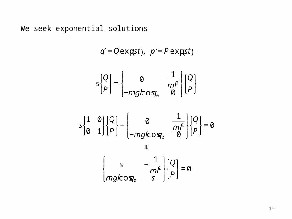
We seek exponential solutions

€

sQ

P

⎧ ⎨ ⎩

⎫ ⎬ ⎭= 0

1

ml2

−mglcosq0 0

⎧ ⎨ ⎪

⎩ ⎪

⎫ ⎬ ⎪

⎭ ⎪

Q

P

⎧ ⎨ ⎩

⎫ ⎬ ⎭€

′ q = Qexp st( ), ′ p = P exp st( )

€

s1 0

0 1

⎧ ⎨ ⎩

⎫ ⎬ ⎭

Q

P

⎧ ⎨ ⎩

⎫ ⎬ ⎭− 0

1

ml2

−mglcosq0 0

⎧ ⎨ ⎪

⎩ ⎪

⎫ ⎬ ⎪

⎭ ⎪

Q

P

⎧ ⎨ ⎩

⎫ ⎬ ⎭= 0

⇓

s −1

ml2

mglcosq0 s

⎧ ⎨ ⎪

⎩ ⎪

⎫ ⎬ ⎪

⎭ ⎪

Q

P

⎧ ⎨ ⎩

⎫ ⎬ ⎭= 0

20

€

det s −1

ml2

mglcosq0 s

⎧ ⎨ ⎪

⎩ ⎪

⎫ ⎬ ⎪

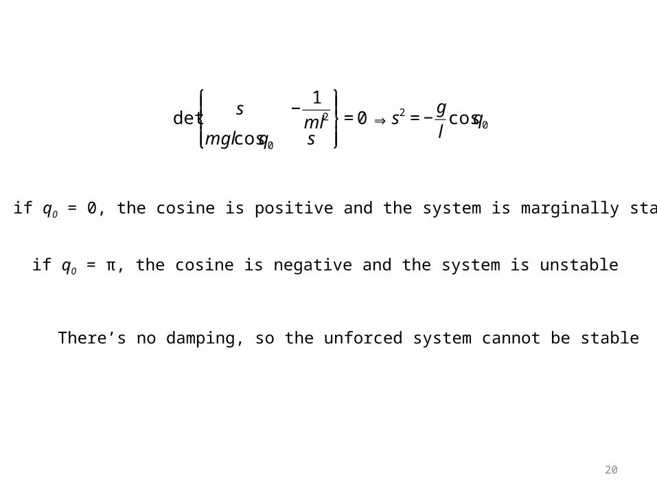
⎭ ⎪= 0⇒ s2 = −

g

lcosq0

if q0 = 0, the cosine is positive and the system is marginally stable

if q0 = π, the cosine is negative and the system is unstable

There’s no damping, so the unforced system cannot be stable

21

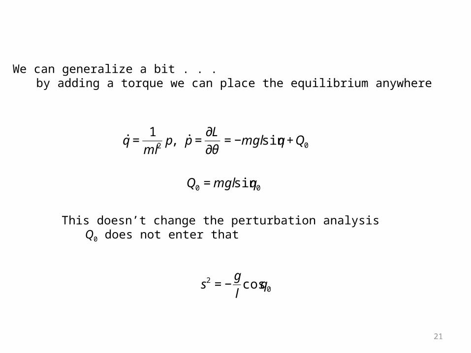
We can generalize a bit . . .by adding a torque we can place the equilibrium anywhere

€

˙ q =1

ml2 p, ˙ p =∂L

∂θ= −mglsinq + Q0

€

Q0 = mglsinq0

This doesn’t change the perturbation analysisQ0 does not enter that

€

s2 = −g

lcosq0

22

The system is unstable if the equilibrium position has q in the second or third quadrants

More colloquially: if the pendulum is above the horizontal

We can illustrate this more physically by an artificial example

23

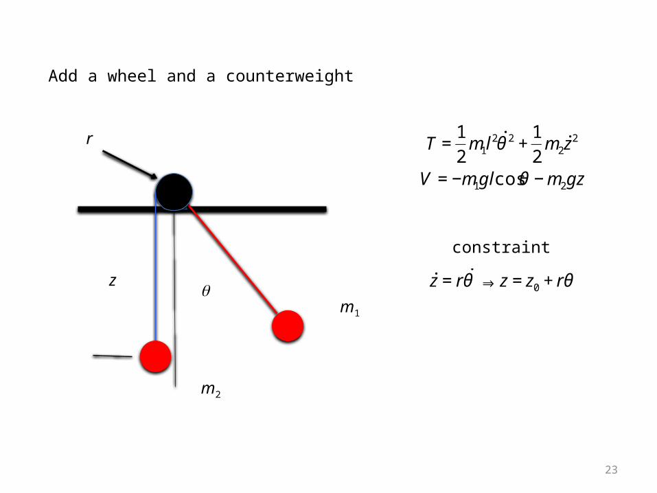
Add a wheel and a counterweight

q m1

m2

r

z€

T =1

2m1l

2 ˙ θ 2 +1

2m2 ˙ z 2

V = −m1glcosθ − m2gz

€

˙ z = r ˙ θ ⇒ z = z0 + rθ

constraint

24

€

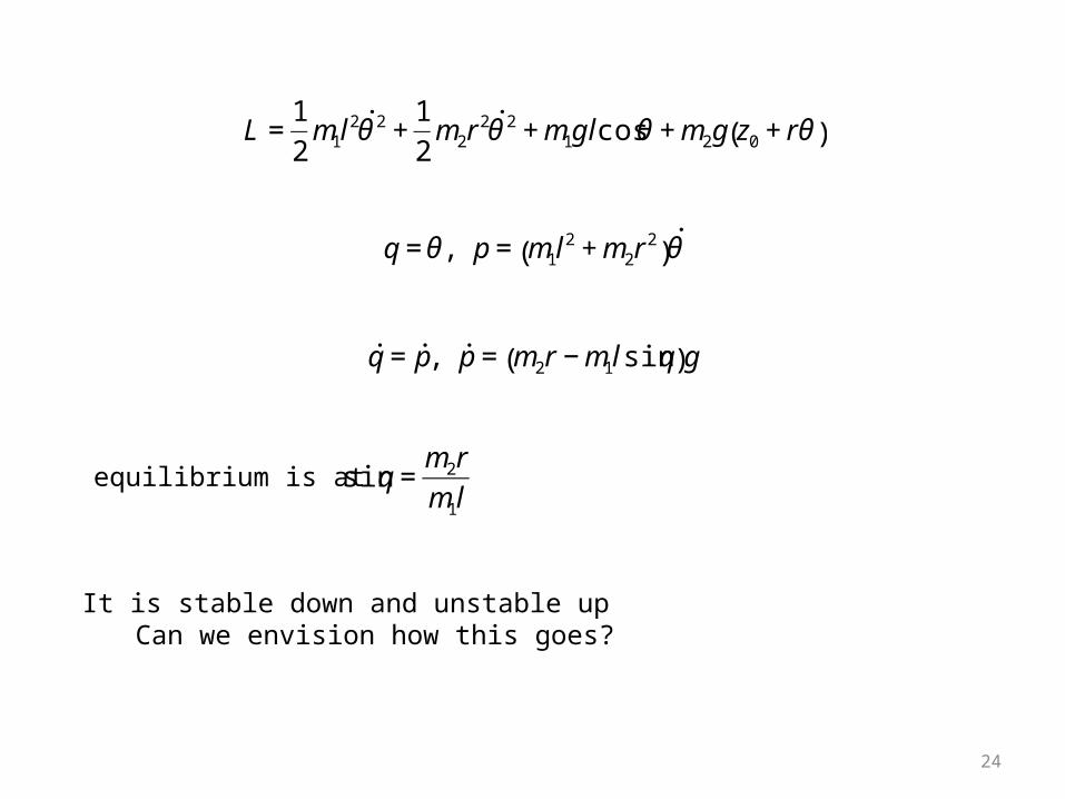
L =1

2m1l

2 ˙ θ 2 +1

2m2r

2 ˙ θ 2 + m1glcosθ + m2g z0 + rθ( )

€

q = θ , p = m1l2 + m2r

2( ) ˙ θ

€

˙ q = ˙ p , ˙ p = m2r − m1lsinq( )g

equilibrium is at

€

sinq =m2r

m1l

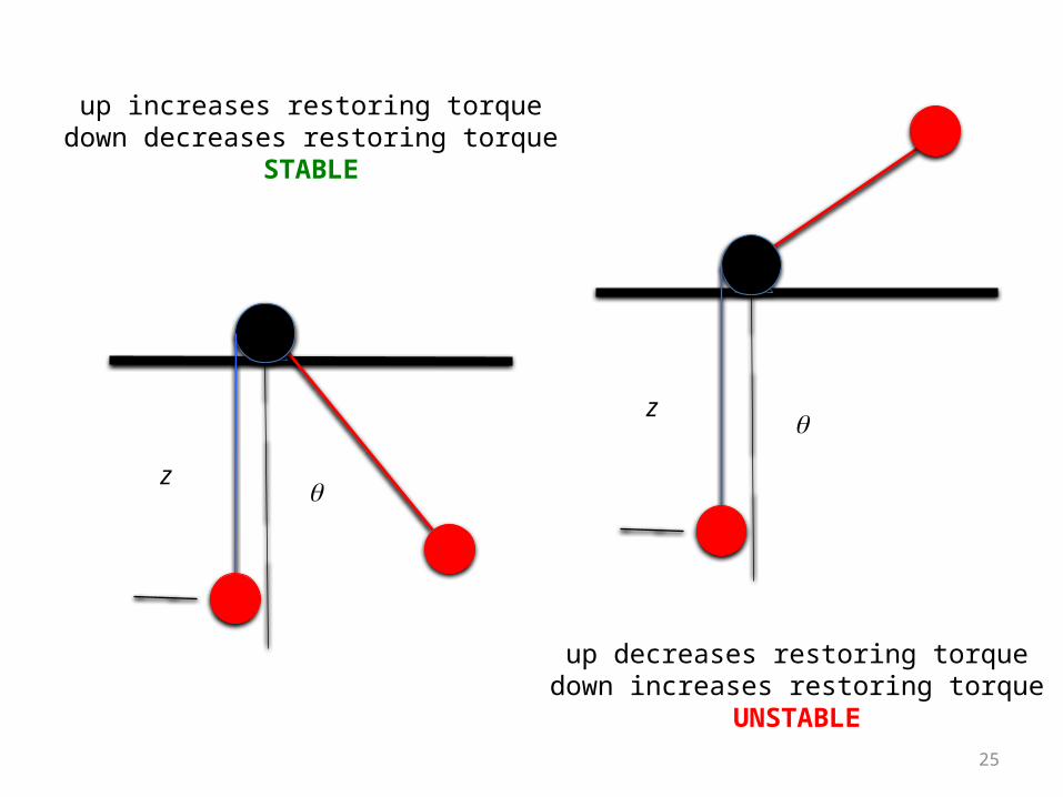
It is stable down and unstable upCan we envision how this goes?

25

qz

up increases restoring torquedown decreases restoring torque

STABLE

qz

up decreases restoring torquedown increases restoring torque

UNSTABLE

26

??

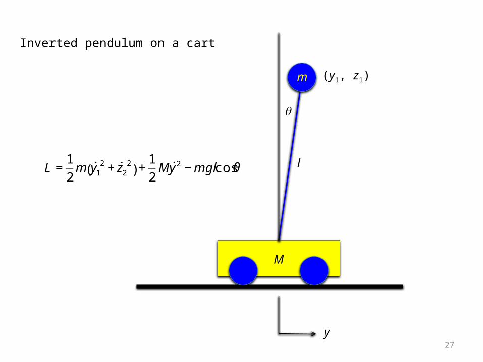
Inverted pendulum on a cart

M

m

l

q

y27

€

L =1

2m ˙ y 1

2 + ˙ z 22

( ) +1

2M˙ y 2 − mglcosθ

(y1, z1)

28

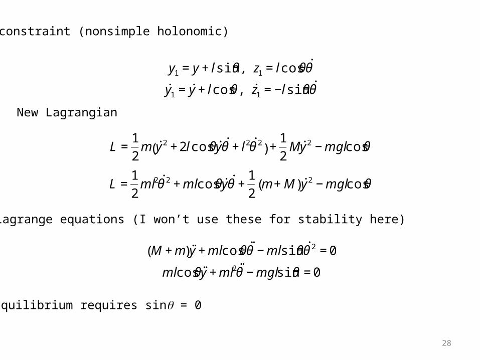
Equilibrium requires sinq = 0

€

y1 = y + lsinθ , z1 = lcosθ ˙ θ

˙ y 1 = ˙ y + lcosθ , ˙ z 1 = −lsinθ ˙ θ

constraint (nonsimple holonomic)

€

M + m( )˙ ̇ y + mlcosθ ˙ ̇ θ − mlsinθ ˙ θ 2 = 0

mlcosθ˙ ̇ y + ml2 ˙ ̇ θ − mglsinθ = 0

Euler-Lagrange equations (I won’t use these for stability here)€

L =1

2m ˙ y 2 + 2lcosθ ˙ y ˙ θ + l2 ˙ θ 2( ) +

1

2M˙ y 2 − mglcosθ

New Lagrangian

€

L =1

2ml2 ˙ θ 2 + mlcosθ ˙ y ˙ θ +

1

2m + M( ) ˙ y 2 − mglcosθ

29

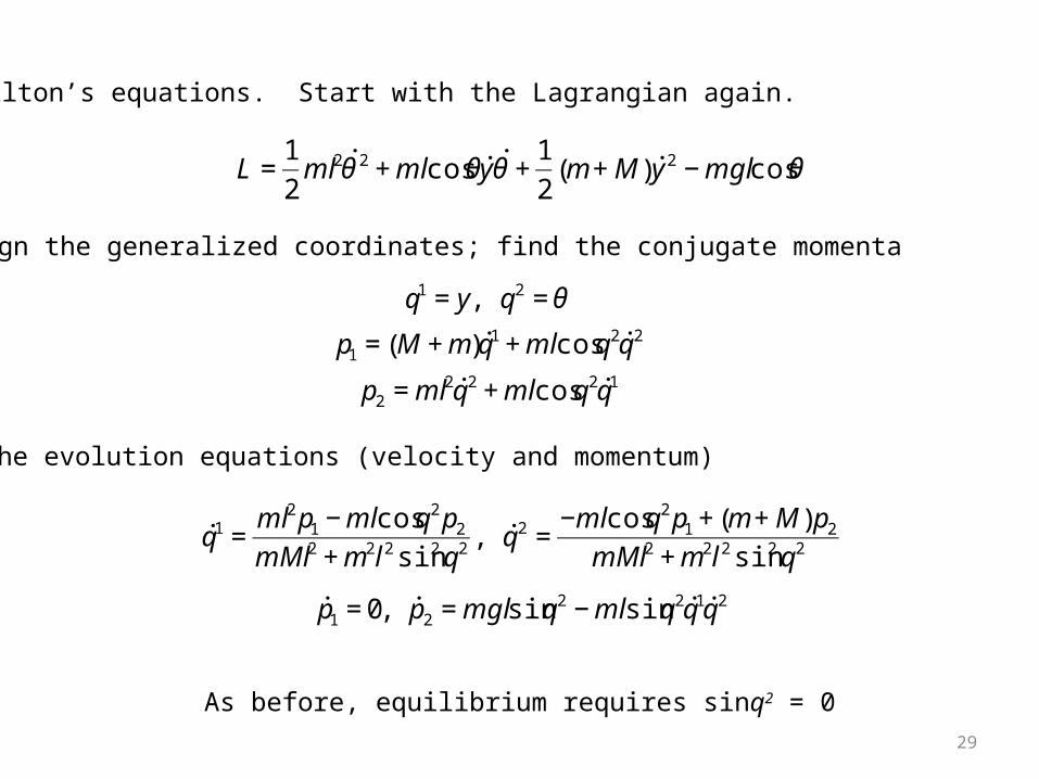
Hamilton’s equations. Start with the Lagrangian again.

€

L =1

2ml2 ˙ θ 2 + mlcosθ ˙ y ˙ θ +

1

2m + M( ) ˙ y 2 − mglcosθ

As before, equilibrium requires sinq2 = 0

€

q1 = y, q2 = θ

p1 = M + m( ) ˙ q 1 + mlcosq2 ˙ q 2

p2 = ml2 ˙ q 2 + mlcosq2 ˙ q 1

assign the generalized coordinates; find the conjugate momenta

€

˙ q 1 =ml2 p1 − mlcosq2 p2

mMl2 + m2l2 sin2 q2 , ˙ q 2 =−mlcosq2 p1 + m + M( )p2

mMl2 + m2l2 sin2 q2

€

˙ p 1 = 0, ˙ p 2 = mglsinq2 − mlsinq2 ˙ q 1˙ q 2

The evolution equations (velocity and momentum)

30

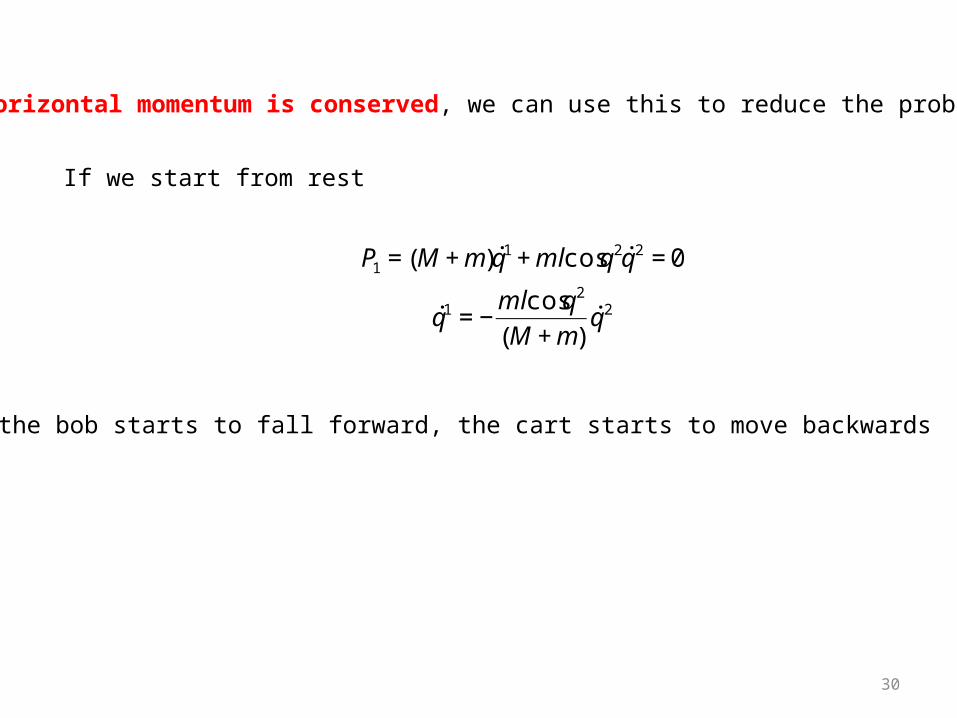
Horizontal momentum is conserved, we can use this to reduce the problem

€

P1 = M + m( ) ˙ q 1 + mlcosq2 ˙ q 2 = 0

˙ q 1 = −mlcosq2

M + m( )˙ q 2

If we start from rest

If the bob starts to fall forward, the cart starts to move backwards

31

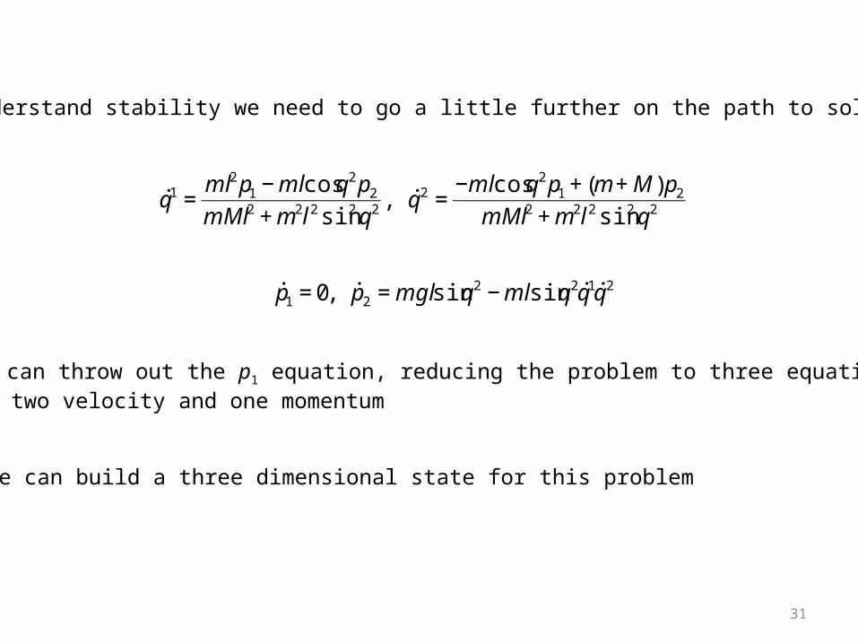
To understand stability we need to go a little further on the path to solution

€

˙ q 1 =ml2 p1 − mlcosq2 p2

mMl2 + m2l2 sin2 q2 , ˙ q 2 =−mlcosq2 p1 + m + M( )p2

mMl2 + m2l2 sin2 q2

€

˙ p 1 = 0, ˙ p 2 = mglsinq2 − mlsinq2 ˙ q 1˙ q 2

We can throw out the p1 equation, reducing the problem to three equations—two velocity and one momentum

We can build a three dimensional state for this problem

32

€

d

dt

q1

q2

p2

⎧

⎨ ⎪

⎩ ⎪

⎫

⎬ ⎪

⎭ ⎪=

ml2 p1 − mlcosq2 p2

mMl2 + m2l2 sin2 q2

−mlcosq2 p1 + m + M( ) p2

mMl2 + m2l2 sin2 q2

mglsinq2 − mlsinq2 ˙ q 1˙ q 2

⎧

⎨

⎪ ⎪ ⎪

⎩

⎪ ⎪ ⎪

⎫

⎬

⎪ ⎪ ⎪

⎭

⎪ ⎪ ⎪

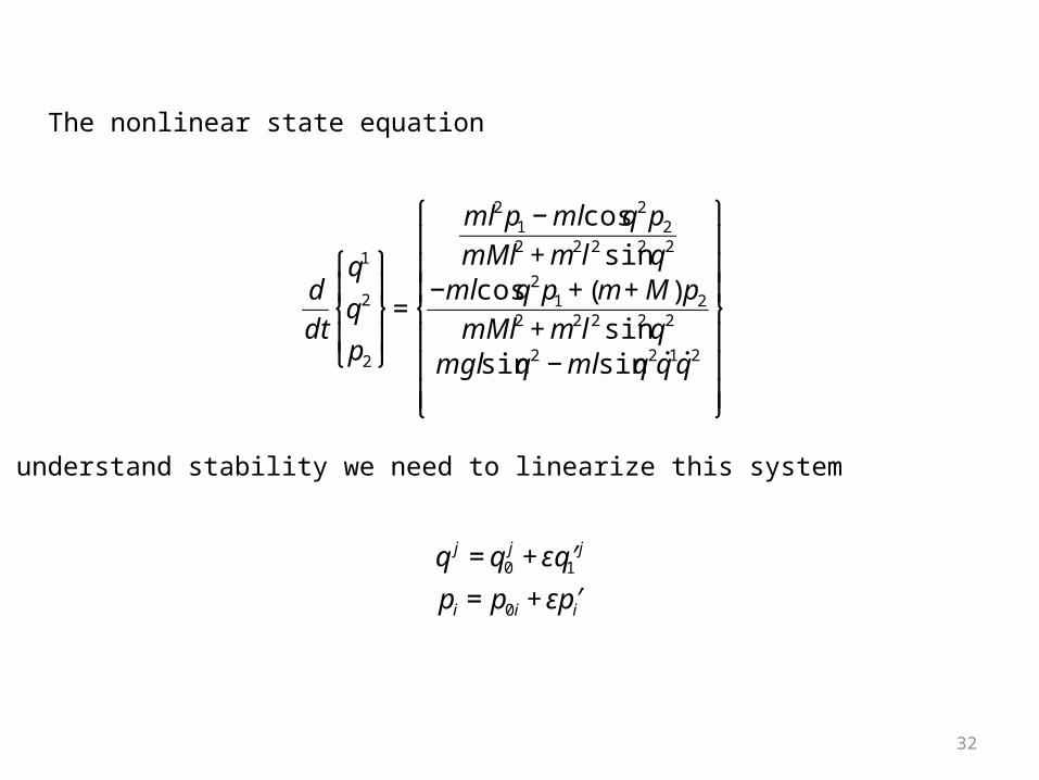
To understand stability we need to linearize this system

€

q j = q0j + ε ′ q 1

j

pi = p0i + ε ′ p i

The nonlinear state equation

33

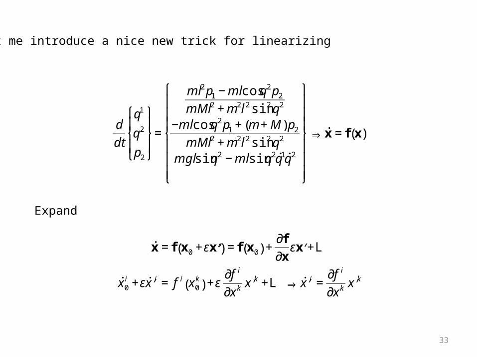
Let me introduce a nice new trick for linearizing

€

d

dt

q1

q2

p2

⎧

⎨ ⎪

⎩ ⎪

⎫

⎬ ⎪

⎭ ⎪=

ml2 p1 − mlcosq2 p2

mMl2 + m2l2 sin2 q2

−mlcosq2 p1 + m + M( ) p2

mMl2 + m2l2 sin2 q2

mglsinq2 − mlsinq2 ˙ q 1˙ q 2

⎧

⎨

⎪ ⎪ ⎪

⎩

⎪ ⎪ ⎪

⎫

⎬

⎪ ⎪ ⎪

⎭

⎪ ⎪ ⎪

⇒ ˙ x = f x( )

€

˙ x = f x0 +ε ′ ′ x ( ) = f x0( ) +∂f

∂xε ′ x +L

˙ x 0i +ε ˙ ′ x i = f i x0

k( ) +ε

∂f i

∂x k ′ x k +L ⇒ ˙ ′ x i =∂f i

∂x k ′ x k

Expand

34

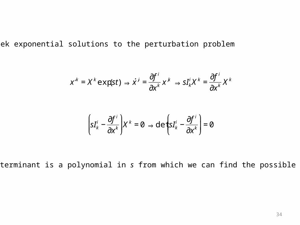
Seek exponential solutions to the perturbation problem

€

′ x k = X k exp st( )⇒ ˙ ′ x i =∂f i

∂x k ′ x k ⇒ sIki X k =

∂f i

∂x k X k

€

sIki −

∂f i

∂x k

⎛

⎝ ⎜

⎞

⎠ ⎟X k = 0⇒ det sIk

i −∂f i

∂x k

⎛

⎝ ⎜

⎞

⎠ ⎟= 0

The determinant is a polynomial in s from which we can find the possible values

35

€

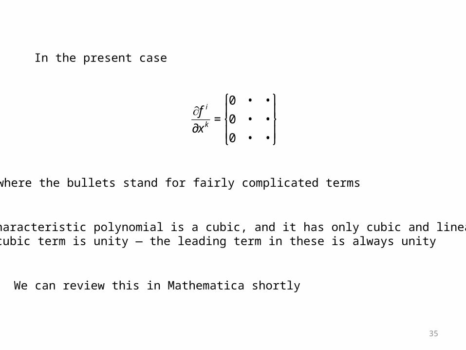
∂f i

∂x k =

0 • •

0 • •

0 • •

⎧

⎨ ⎪

⎩ ⎪

⎫

⎬ ⎪

⎭ ⎪

where the bullets stand for fairly complicated terms

The characteristic polynomial is a cubic, and it has only cubic and linear terms(the cubic term is unity — the leading term in these is always unity

We can review this in Mathematica shortly

In the present case

36

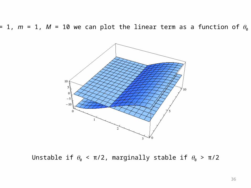
For l = 1, m = 1, M = 10 we can plot the linear term as a function of q0 and p1

Unstable if q0 < π/2, marginally stable if q0 > π/2

37

??

38

What about something a little more real: the three link robot.

We’ll look at this one in Mathematica as well, but we can say some things

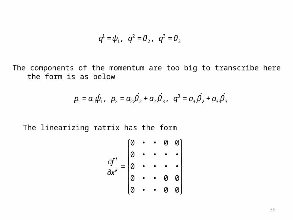
Recall that we have three generalized coordinates after applying all the holonomic constraints

39

€

q1 =ψ1, q2 = θ 2, q

3 = θ 3

€

∂f i

∂x k =

0 • • 0 0

0 • • • •

0 • • • •

0 • • 0 0

0 • • 0 0

⎧

⎨

⎪ ⎪ ⎪

⎩

⎪ ⎪ ⎪

⎫

⎬

⎪ ⎪ ⎪

⎭

⎪ ⎪ ⎪

The components of the momentum are too big to transcribe herethe form is as below

€

p1 = a11˙ ψ 1, p2 = a22

˙ θ 2 + a23˙ θ 3, q

3 = a32˙ θ 2 + a33

˙ θ 3

The linearizing matrix has the form

40

The characteristic polynomial is a quintic equation with no constant term

The zero eigenvalue means that we are at best marginally stable

All but the quintic and cubic terms drop out when the robot is stationaryso I have three zero eigenvalues and two nonzero eigenvalues

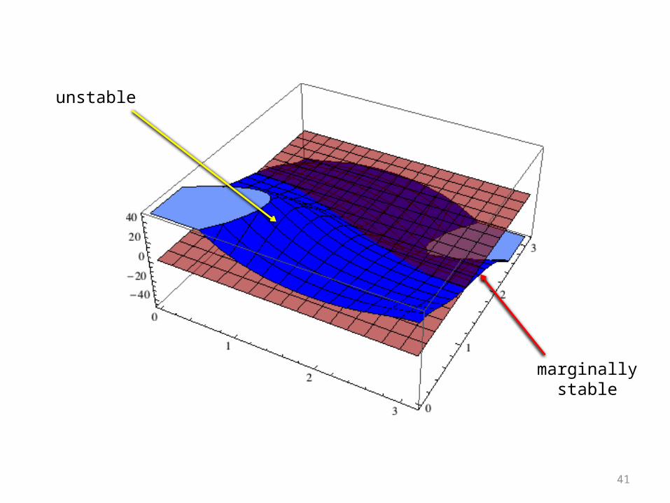
I can plot their square

41

unstable

marginallystable

42

??On to Mathematica: the inverted pendulum and the three-link robot