Lecture 12

Brian Caffo

Table ofcontents

Outline

The jackknife

The bootstrapprinciple

The bootstrap

Lecture 12

Brian Caffo

Department of BiostatisticsJohns Hopkins Bloomberg School of Public Health

Johns Hopkins University

August 23, 2007

Lecture 12

Brian Caffo

Table ofcontents

Outline

The jackknife

The bootstrapprinciple

The bootstrap

Table of contents

1 Table of contents

2 Outline

3 The jackknife

4 The bootstrap principle

5 The bootstrap

Lecture 12

Brian Caffo

Table ofcontents

Outline

The jackknife

The bootstrapprinciple

The bootstrap

Outline

1 The jackknife

2 Introduce the bootstrap principle

3 Outline the bootstrap algorithm

4 Example bootstrap calculations

5 Discussion

Lecture 12

Brian Caffo

Table ofcontents

Outline

The jackknife

The bootstrapprinciple

The bootstrap

The jackknife

• The jackknife is a tool for estimating standard errors andthe bias of estimators

• As its name suggests, the jackknife is a small, handy tool;in contrast to the bootstrap, which is then the moralequivalent of a giant workshop full of tools

• Both the jackknife and the bootstrap involve resamplingdata; that is, repeatedly creating new data sets from theoriginal data

Lecture 12

Brian Caffo

Table ofcontents

Outline

The jackknife

The bootstrapprinciple

The bootstrap

The jackknife

• The jackknife deletes each observation and calculates anestimate based on the remaining n − 1 of them

• It uses this collection of estimates to do things likeestimate the bias and the standard error

• Note that estimating the bias and having a standard errorare not needed for things like sample means, which weknow are unbiased estimates of population means andwhat their standard errors are

Lecture 12

Brian Caffo

Table ofcontents

Outline

The jackknife

The bootstrapprinciple

The bootstrap

The jackknife

• We’ll consider the jackknife for univariate data

• Let X1, . . . ,Xn be a collection of data used to estimate aparameter θ

• Let θ̂ be the estimate based on the full data set

• Let θ̂i be the estimate of θ obtained by deletingobservation i

• Let θ̄ = 1n

∑ni=1 θ̂i

Lecture 12

Brian Caffo

Table ofcontents

Outline

The jackknife

The bootstrapprinciple

The bootstrap

Continued

• Then, the jackknife estimate of the bias is

(n − 1)(θ̄ − θ̂

)(how far the average delete-one estimate is from theactual estimate)

• The jackknife estimate of the standard error is[n − 1

n

n∑i=1

(θ̂i − θ̄)2

]1/2

(the deviance of the delete-one estimates from the averagedelete-one estimate)

Lecture 12

Brian Caffo

Table ofcontents

Outline

The jackknife

The bootstrapprinciple

The bootstrap

Example

• Consider the data set of 630 measurements of gray mattervolume for workers from a lead manufacturing plant

• The median gray matter volume is around 589 cubiccentimeters

• We want to estimate the bias and standard error of themedian

Lecture 12

Brian Caffo

Table ofcontents

Outline

The jackknife

The bootstrapprinciple

The bootstrap

Example

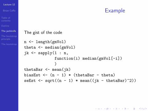
The gist of the code

n <- length(gmVol)theta <- median(gmVol)jk <- sapply(1 : n,

function(i) median(gmVol[-i]))

thetaBar <- mean(jk)biasEst <- (n - 1) * (thetaBar - theta)seEst <- sqrt((n - 1) * mean((jk - thetaBar)^2))

Lecture 12

Brian Caffo

Table ofcontents

Outline

The jackknife

The bootstrapprinciple

The bootstrap

Example

Or, using the bootstrap package

library(bootstrap)out <- jackknife(gmVol, median)out$jack.seout$jack.bias

Lecture 12

Brian Caffo

Table ofcontents

Outline

The jackknife

The bootstrapprinciple

The bootstrap

Example

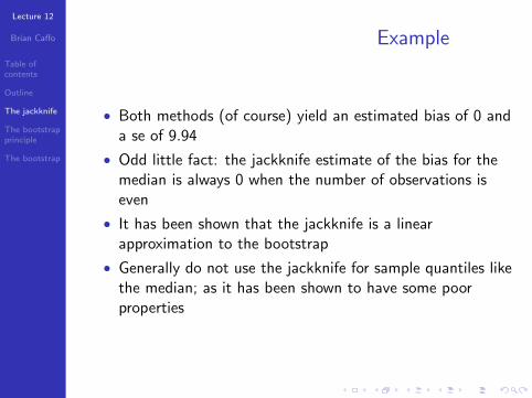
• Both methods (of course) yield an estimated bias of 0 anda se of 9.94

• Odd little fact: the jackknife estimate of the bias for themedian is always 0 when the number of observations iseven

• It has been shown that the jackknife is a linearapproximation to the bootstrap

• Generally do not use the jackknife for sample quantiles likethe median; as it has been shown to have some poorproperties

Lecture 12

Brian Caffo

Table ofcontents

Outline

The jackknife

The bootstrapprinciple

The bootstrap

Pseudo observations

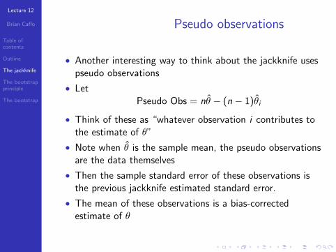
• Another interesting way to think about the jackknife usespseudo observations

• LetPseudo Obs = nθ̂ − (n − 1)θ̂i

• Think of these as “whatever observation i contributes tothe estimate of θ”

• Note when θ̂ is the sample mean, the pseudo observationsare the data themselves

• Then the sample standard error of these observations isthe previous jackknife estimated standard error.

• The mean of these observations is a bias-correctedestimate of θ

Lecture 12

Brian Caffo

Table ofcontents

Outline

The jackknife

The bootstrapprinciple

The bootstrap

Example: Tom’s notes

Lecture 12

Brian Caffo

Table ofcontents

Outline

The jackknife

The bootstrapprinciple

The bootstrap

The bootstrap

• The bootstrap is a tremendously useful tool forconstructing confidence intervals and calculating standarderrors for difficult statistics

• For example, how would one derive a confidence intervalfor the median?

• The bootstrap procedure follows from the so calledbootstrap principle

Lecture 12

Brian Caffo

Table ofcontents

Outline

The jackknife

The bootstrapprinciple

The bootstrap

The bootstrap principle

• Suppose that I have a statistic that estimates somepopulation parameter, but I don’t know its samplingdistribution

• The bootstrap principle suggests using the distributiondefined by the data to approximate its samplingdistribution

Lecture 12

Brian Caffo

Table ofcontents

Outline

The jackknife

The bootstrapprinciple

The bootstrap

The bootstrap in practice

• In practice, the bootstrap principle is always carried outusing simulation

• We will cover only a few aspects of bootstrap resampling

• The general procedure follows by first simulating completedata sets from the observed data with replacement

• This is approximately drawing from the samplingdistribution of that statistic, at least as far as the data isable to approximate the true population distribution

• Calculate the statistic for each simulated data set

• Use the simulated statistics to either define a confidenceinterval or take the standard deviation to calculate astandard error

Lecture 12

Brian Caffo

Table ofcontents

Outline

The jackknife

The bootstrapprinciple

The bootstrap

Example

• Consider again, the data set of 630 measurements of graymatter volume for workers from a lead manufacturing plant

• The median gray matter volume is around 589 cubiccentimeters

• We want a confidence interval for the median of thesemeasurements

Lecture 12

Brian Caffo

Table ofcontents

Outline

The jackknife

The bootstrapprinciple

The bootstrap

• Bootstrap procedure for calculating for the median from adata set of n observations

i . Sample n observations with replacement from theobserved data resulting in one simulated complete data set

ii . Take the median of the simulated data setiii . Repeat these two steps B times, resulting in B simulated

mediansiv . These medians are approximately draws from the sampling

distribution of the median of n observations; therefore wecan

• Draw a histogram of them• Calculate their standard deviation to estimate the

standard error of the median• Take the 2.5th and 97.5th percentiles as a confidence

interval for the median

Lecture 12

Brian Caffo

Table ofcontents

Outline

The jackknife

The bootstrapprinciple

The bootstrap

Example code

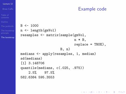
B <- 1000n <- length(gmVol)resamples <- matrix(sample(gmVol,

n * B,replace = TRUE),

B, n)medians <- apply(resamples, 1, median)sd(medians)[1] 3.148706quantile(medians, c(.025, .975))

2.5% 97.5%582.6384 595.3553

Lecture 12

Brian Caffo

Table ofcontents

Outline

The jackknife

The bootstrapprinciple

The bootstrap

580 585 590 595 600 605

0.00

0.05

0.10

0.15

Gray Matter Volume

dens

ity

Lecture 12

Brian Caffo

Table ofcontents

Outline

The jackknife

The bootstrapprinciple

The bootstrap

Notes on the bootstrap

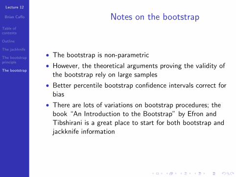
• The bootstrap is non-parametric

• However, the theoretical arguments proving the validity ofthe bootstrap rely on large samples

• Better percentile bootstrap confidence intervals correct forbias

• There are lots of variations on bootstrap procedures; thebook “An Introduction to the Bootstrap” by Efron andTibshirani is a great place to start for both bootstrap andjackknife information

Lecture 12

Brian Caffo

Table ofcontents

Outline

The jackknife

The bootstrapprinciple

The bootstrap

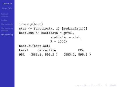
library(boot)stat <- function(x, i) {median(x[i])}boot.out <- boot(data = gmVol,

statistic = stat,R = 1000)

boot.ci(boot.out)Level Percentile BCa95% (583.1, 595.2 ) (583.2, 595.3 )