Lecture – 11 - NPTELtextofvideo.nptel.ac.in/117102060/lec11.pdf · Lecture - 11 . Discrete Fourier Transform (DFT Cont.) ... How to calculate linear convolution if the two sequences

Digital Signal Processing

Prof. S. C. Dutta Roy

Department of Electrical Engineering

Indian Institute of Technology, Delhi

Lecture - 11

Discrete Fourier Transform (DFT Cont.)

Introduction to Z-transform

This is the 11th lecture on DSP and today we continue our discussion on Discrete Fourier

Transform and then we introduce the Z-transform. In the last lecture, we started with the

determination of the spectrum of a given signal by DFT. The signal is given for n = 0 to N – 1,

and you want the spectrum at a dense set of frequencies; what you do is that you add the required

number of 0s so that the total length becomes M, where M may be much larger than N. Then you

compute the DFT. We also discussed the properties of DFT such as linearity and circular shift

and I illustrated the latter with a circle diagram. The other properties were modulation and

Parseval’s relation. The computation of circular convolution is extremely important because it is

an aid to calculating linear convolution.

Most of the time, you shall have to calculate linear convolution, that is response of a given

system to a given input, and that is linear convolution. Circular convolution is a contrived

technique because it helps in finding linear convolution by FFT. That is the only use of circular

convolution. We discussed several methods of circular convolution: Graphical method was

followed by mechanization in the form of a table and multiplication and addition. We also

discussed how to calculate circular convolution from DFT. We multiply the two DFTs and take

the IDFT of the product. This can be done from the summation or its matrix representation. The

matrix form happens to be easier sometimes, but not all the time.

How to calculate linear convolution if the two sequences have different lengths N and M? You

first find out what the length of the linear convolution shall be. It will be N + M – 1 = L, say.

Then you add 0s to both the sequences to make each of them of length L and then calculate the

circular convolution; that will give you the desired linear convolution. There is yet another

1

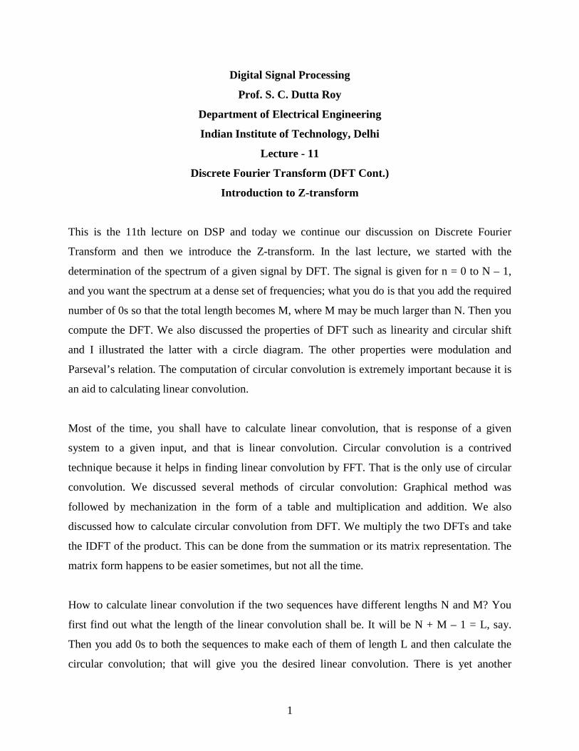
method for calculating circular convolution, by taking help of what is known as the Circulant

Matrix.

(Refer Slide Time: 04:02 - 05:56)

This is a reflection of circular shift. You recall that, if I have to calculate y(n) which is g(n)

circularly convolved at N number of points with h(n), then the required relationship is

summation[g(m) h(n – m)N] where m goes from 0 to N – 1. Let us expand this relationship for a

few samples of the output. The first sample y(0) becomes g(0) h(0) + g(1)h(N – 1) + g(2) h(N –

2) and so on up to g(N – 1) h(1). Remember that h(n – m) has to be taken with module N.

Similarly if I calculate y(1) then it would be g(0) h(1) + g(1)h(0) + g(2)h(N – 1) + …. + g(N –

1)h(2) and we can continue this.

2


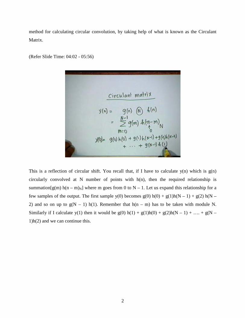
Notice that the sum of the two arguments in y(1) is 0 + 1 in the first term, and N – 1 + 2 = N + 1

which is the same as 1 in the second term. Similar is the case with each term. If you notice this,

then you can easily write y(0) y(1)…..y(N – 1) in a matrix form as the product of a square matrix

―H and a column vector g = [g(0), g(1)….. g(N – 1)]T. The first row is h(0), h(N – 1)…… h(1). In

the next row, we have h(1), h(0), h(N – 1),…. What would be the last sample? The last sample

will be h(2) and this continues. The last row would be h(N – 1), h(N – 2),….h(0). If you can

write the first column as h(0), h(1),…… h(N – 1), then you can write the whole of the matrix.

You see that the main diagonal has all h(0)s.

The matrix is a very interesting one; it is called a Circulant matrix because samples simply

circulate. Once you are able to write this matrix, then you can calculate the circular convolution.

Whatever procedure appears attractive to you, adopt that.

3


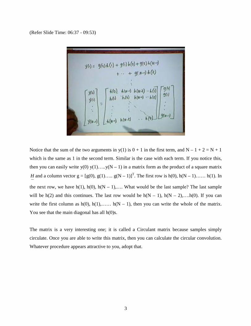
We have two sequences g(n) and h(n) each of length N, N = 0 to N – 1. We wish to calculate

G(k) and H(k). If we wish to calculate both of them normally, it shall require two N point DFTs.

But then if we combine the two signals analytically, that is we put one signal at quadrature with

the other signal, we form a new sequence which is x(n) = g(n) + j h(n), Quadrature means

multiplying by j. In other words, we are making this signal intentionally complex. Now we can

find out the N point DFT of x(n) which is also of length N. We calculate X(k), from which, if

possible we have to extract G(k) and H(k). Now you notice that the g(n) is nothing but (x(n) + x*

(n))/2, x*(n) being the complex conjugate of x(n). Similarly h(n) = [x(n) – x*(n)]/(2j) and

therefore if we calculate X(k) and the DFT of x*(n) then we can find out G(k) and H(k).

4


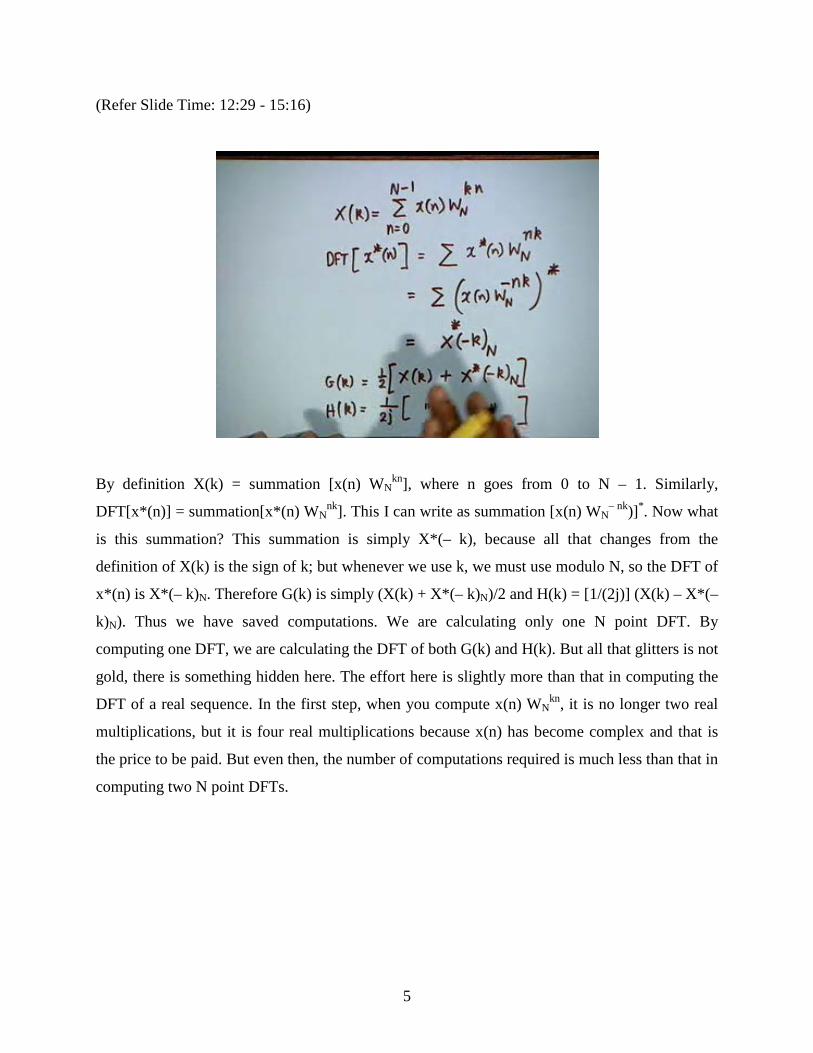
By definition X(k) = summation [x(n) WNkn], where n goes from 0 to N – 1. Similarly,

DFT[x*(n)] = summation[x*(n) WNnk]. This I can write as summation [x(n) WN

– nk)]*. Now what

is this summation? This summation is simply X*(– k), because all that changes from the

definition of X(k) is the sign of k; but whenever we use k, we must use modulo N, so the DFT of

x*(n) is X*(– k)N. Therefore G(k) is simply (X(k) + X*(– k)N)/2 and H(k) = [1/(2j)] (X(k) – X*(–

k)N). Thus we have saved computations. We are calculating only one N point DFT. By

computing one DFT, we are calculating the DFT of both G(k) and H(k). But all that glitters is not

gold, there is something hidden here. The effort here is slightly more than that in computing the

DFT of a real sequence. In the first step, when you compute x(n) WNkn, it is no longer two real

multiplications, but it is four real multiplications because x(n) has become complex and that is

the price to be paid. But even then, the number of computations required is much less than that in

computing two N point DFTs.

5


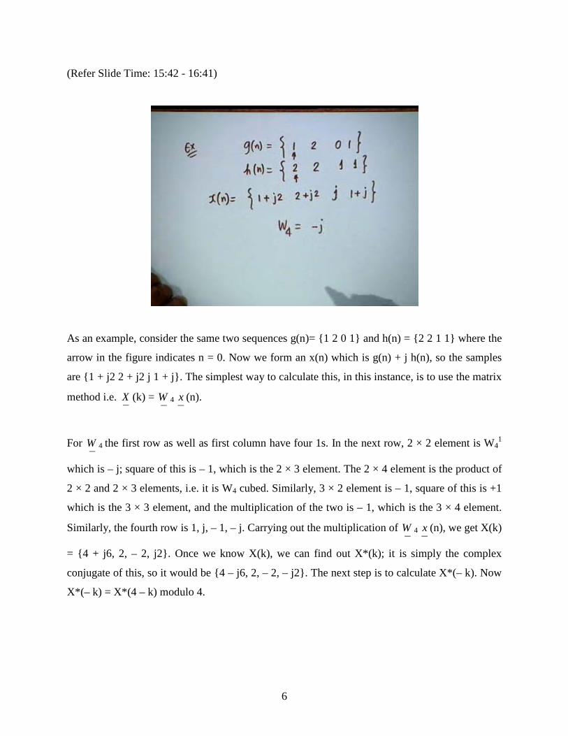
As an example, consider the same two sequences g(n)= {1 2 0 1} and h(n) = {2 2 1 1} where the

arrow in the figure indicates n = 0. Now we form an x(n) which is g(n) + j h(n), so the samples

are {1 + j2 2 + j2 j 1 + j}. The simplest way to calculate this, in this instance, is to use the matrix

method i.e. ―X (k) =

―W 4

―x (n).

For ―W 4 the first row as well as first column have four 1s. In the next row, 2 × 2 element is W4

1

which is – j; square of this is – 1, which is the 2 × 3 element. The 2 × 4 element is the product of

2 × 2 and 2 × 3 elements, i.e. it is W4 cubed. Similarly, 3 × 2 element is – 1, square of this is +1

which is the 3 × 3 element, and the multiplication of the two is – 1, which is the 3 × 4 element.

Similarly, the fourth row is 1, j, – 1, – j. Carrying out the multiplication of ―W 4

―x (n), we get X(k)

= {4 + j6, 2, – 2, j2}. Once we know X(k), we can find out X*(k); it is simply the complex

conjugate of this, so it would be {4 – j6, 2, – 2, – j2}. The next step is to calculate X*(– k). Now

X*(– k) = X*(4 – k) modulo 4.

6


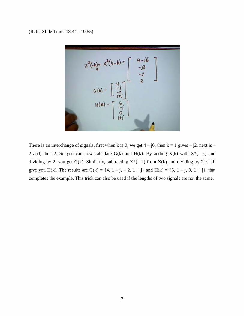
There is an interchange of signals, first when k is 0, we get 4 – j6; then k = 1 gives – j2, next is –

2 and, then 2. So you can now calculate G(k) and H(k). By adding X(k) with X*(– k) and

dividing by 2, you get G(k). Similarly, subtracting X*(– k) from X(k) and dividing by 2j shall

give you H(k). The results are G(k) = {4, 1 – j, – 2, 1 + j} and H(k) = {6, 1 – j, 0, 1 + j}; that

completes the example. This trick can also be used if the lengths of two signals are not the same.

7


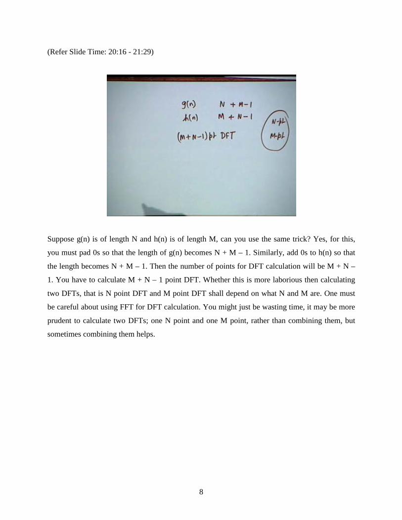
Suppose g(n) is of length N and h(n) is of length M, can you use the same trick? Yes, for this,

you must pad 0s so that the length of g(n) becomes N + M – 1. Similarly, add 0s to h(n) so that

the length becomes N + M – 1. Then the number of points for DFT calculation will be M + N –

1. You have to calculate M + N – 1 point DFT. Whether this is more laborious then calculating

two DFTs, that is N point DFT and M point DFT shall depend on what N and M are. One must

be careful about using FFT for DFT calculation. You might just be wasting time, it may be more

prudent to calculate two DFTs; one N point and one M point, rather than combining them, but

sometimes combining them helps.

8


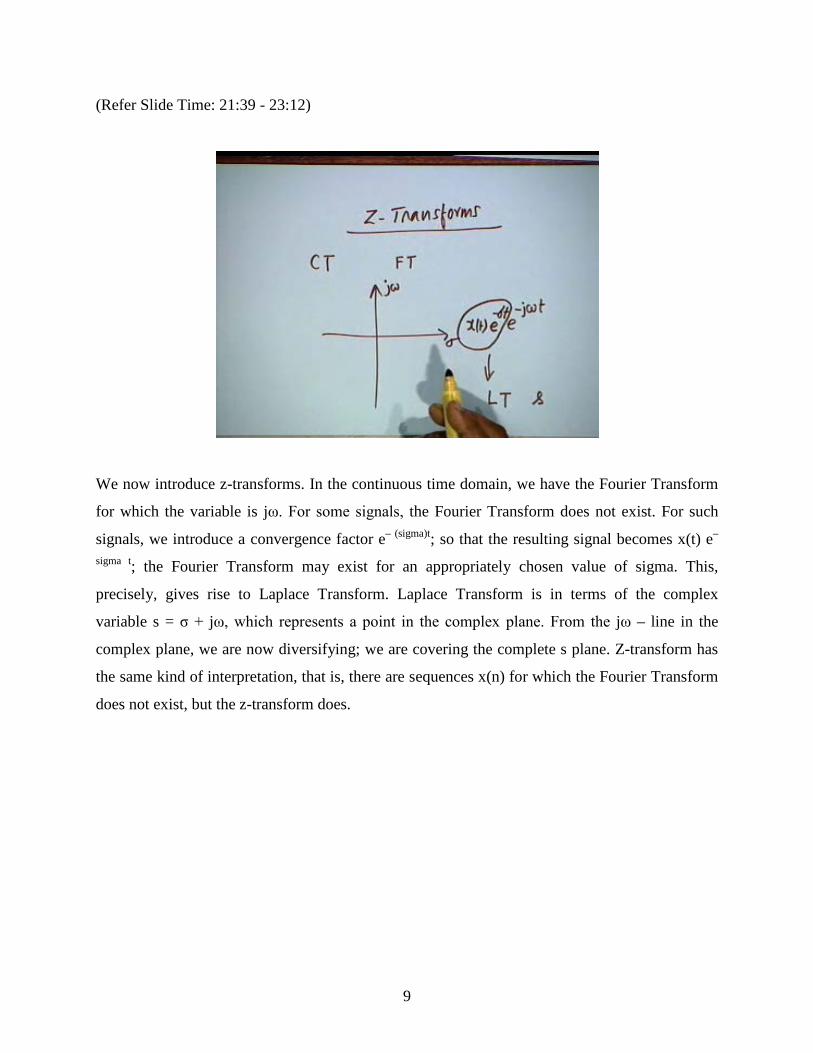
We now introduce z-transforms. In the continuous time domain, we have the Fourier Transform

for which the variable is jω. For some signals, the Fourier Transform does not exist. For such

signals, we introduce a convergence factor e– (sigma)t; so that the resulting signal becomes x(t) e–

sigma t; the Fourier Transform may exist for an appropriately chosen value of sigma. This,

precisely, gives rise to Laplace Transform. Laplace Transform is in terms of the complex

variable s = σ + jω, which represents a point in the complex plane. From the jω – line in the

complex plane, we are now diversifying; we are covering the complete s plane. Z-transform has

the same kind of interpretation, that is, there are sequences x(n) for which the Fourier Transform

does not exist, but the z-transform does.

9


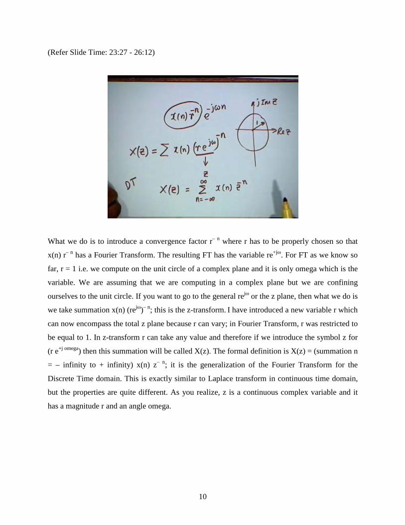
What we do is to introduce a convergence factor r– n where r has to be properly chosen so that

x(n) r– n has a Fourier Transform. The resulting FT has the variable re+jω. For FT as we know so

far, r = 1 i.e. we compute on the unit circle of a complex plane and it is only omega which is the

variable. We are assuming that we are computing in a complex plane but we are confining

ourselves to the unit circle. If you want to go to the general rejω or the z plane, then what we do is

we take summation x(n) (rejω)– n; this is the z-transform. I have introduced a new variable r which

can now encompass the total z plane because r can vary; in Fourier Transform, r was restricted to

be equal to 1. In z-transform r can take any value and therefore if we introduce the symbol z for

(r e+j omega) then this summation will be called X(z). The formal definition is X(z) = (summation n

= – infinity to + infinity) x(n) z– n; it is the generalization of the Fourier Transform for the

Discrete Time domain. This is exactly similar to Laplace transform in continuous time domain,

but the properties are quite different. As you realize, z is a continuous complex variable and it

has a magnitude r and an angle omega.

10


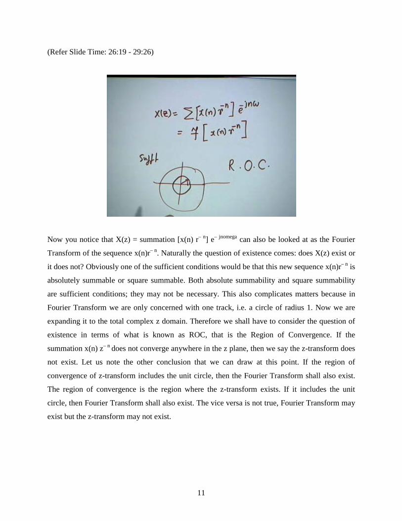
Now you notice that X(z) = summation [x(n) r– n] e– jnomega can also be looked at as the Fourier

Transform of the sequence x(n)r– n. Naturally the question of existence comes: does X(z) exist or

it does not? Obviously one of the sufficient conditions would be that this new sequence x(n)r– n is

absolutely summable or square summable. Both absolute summability and square summability

are sufficient conditions; they may not be necessary. This also complicates matters because in

Fourier Transform we are only concerned with one track, i.e. a circle of radius 1. Now we are

expanding it to the total complex z domain. Therefore we shall have to consider the question of

existence in terms of what is known as ROC, that is the Region of Convergence. If the

summation x(n) z– n does not converge anywhere in the z plane, then we say the z-transform does

not exist. Let us note the other conclusion that we can draw at this point. If the region of

convergence of z-transform includes the unit circle, then the Fourier Transform shall also exist.

The region of convergence is the region where the z-transform exists. If it includes the unit

circle, then Fourier Transform shall also exist. The vice versa is not true, Fourier Transform may

exist but the z-transform may not exist.

11


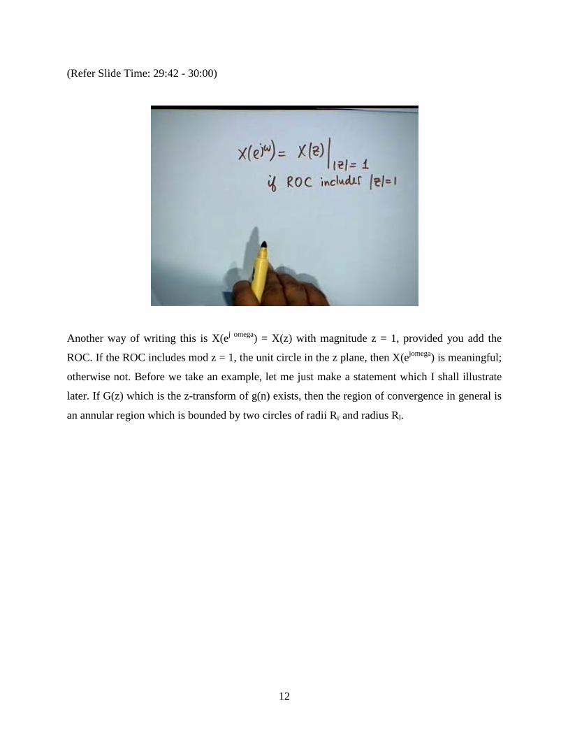
Another way of writing this is X(ej omega) = X(z) with magnitude z = 1, provided you add the

ROC. If the ROC includes mod z = 1, the unit circle in the z plane, then X(ejomega) is meaningful;

otherwise not. Before we take an example, let me just make a statement which I shall illustrate

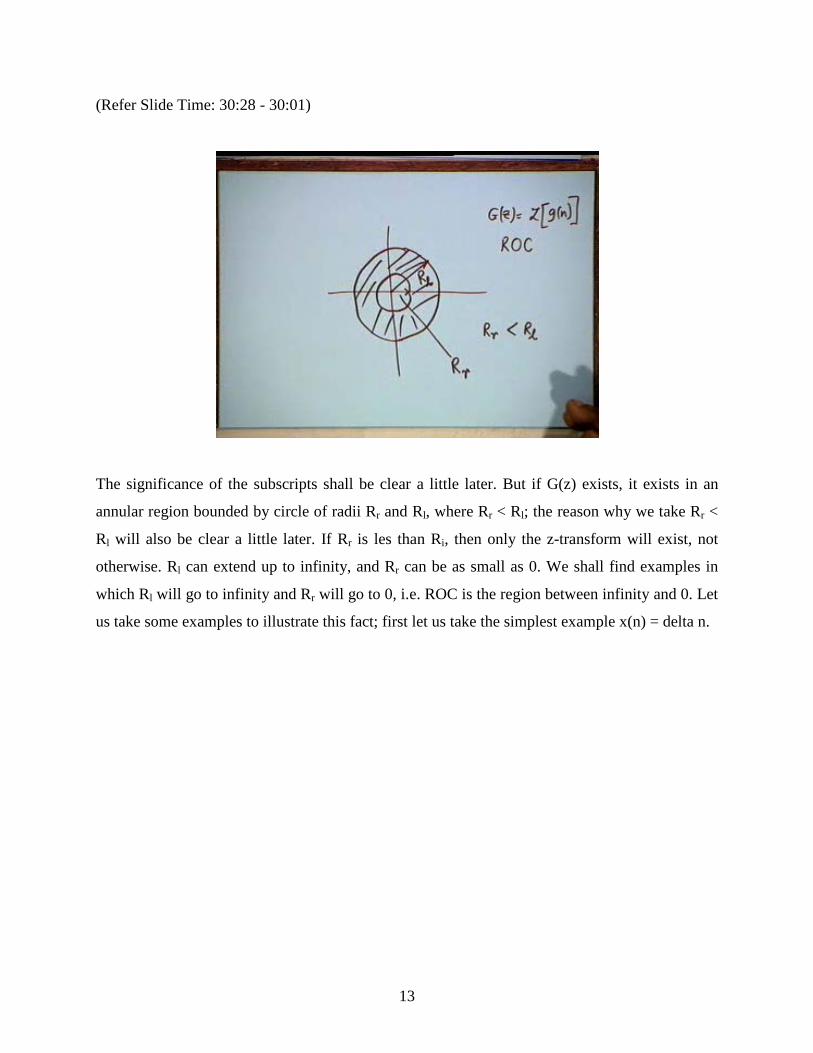
later. If G(z) which is the z-transform of g(n) exists, then the region of convergence in general is

an annular region which is bounded by two circles of radii Rr and radius Rl.

12


The significance of the subscripts shall be clear a little later. But if G(z) exists, it exists in an

annular region bounded by circle of radii Rr and Rl, where Rr < Rl; the reason why we take Rr <

Rl will also be clear a little later. If Rr is les than Ri, then only the z-transform will exist, not

otherwise. Rl can extend up to infinity, and Rr can be as small as 0. We shall find examples in

which Rl will go to infinity and Rr will go to 0, i.e. ROC is the region between infinity and 0. Let

us take some examples to illustrate this fact; first let us take the simplest example x(n) = delta n.

13


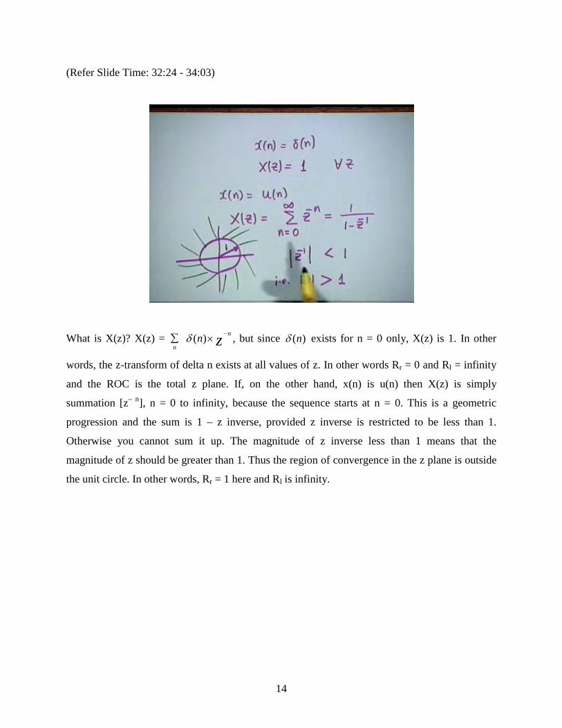
What is X(z)? X(z) = n∑ ( ) nn zδ −× , but since ( )nδ exists for n = 0 only, X(z) is 1. In other

words, the z-transform of delta n exists at all values of z. In other words Rr = 0 and Rl = infinity

and the ROC is the total z plane. If, on the other hand, x(n) is u(n) then X(z) is simply

summation [z– n], n = 0 to infinity, because the sequence starts at n = 0. This is a geometric

progression and the sum is 1 – z inverse, provided z inverse is restricted to be less than 1.

Otherwise you cannot sum it up. The magnitude of z inverse less than 1 means that the

magnitude of z should be greater than 1. Thus the region of convergence in the z plane is outside

the unit circle. In other words, Rr = 1 here and Rl is infinity.

14


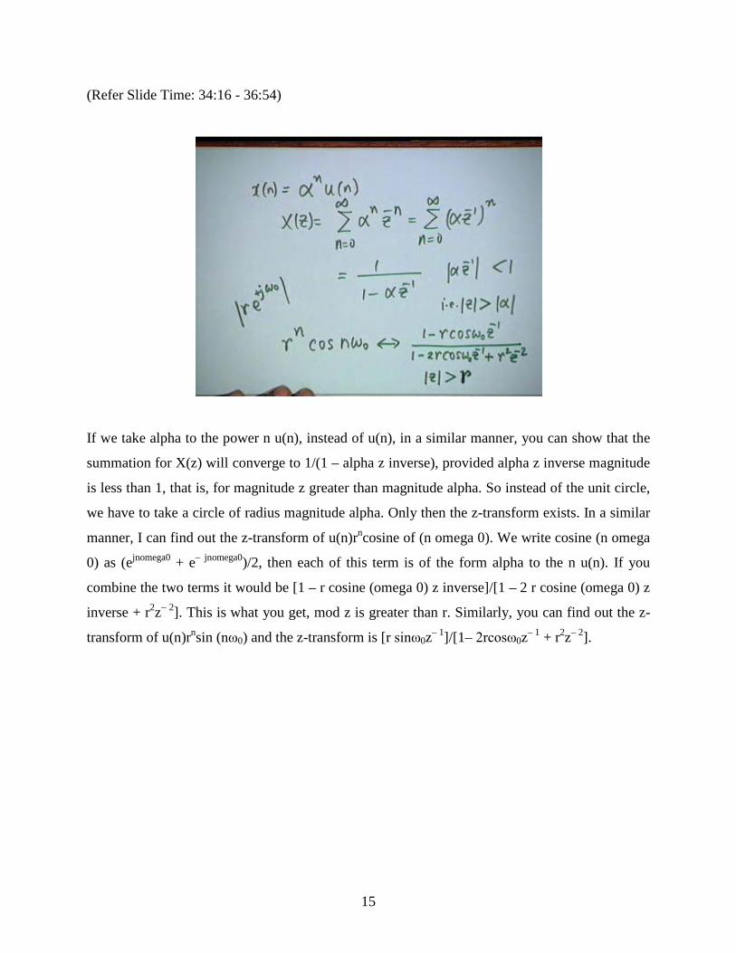
If we take alpha to the power n u(n), instead of u(n), in a similar manner, you can show that the

summation for X(z) will converge to 1/(1 – alpha z inverse), provided alpha z inverse magnitude

is less than 1, that is, for magnitude z greater than magnitude alpha. So instead of the unit circle,

we have to take a circle of radius magnitude alpha. Only then the z-transform exists. In a similar

manner, I can find out the z-transform of u(n)rncosine of (n omega 0). We write cosine (n omega

0) as (ejnomega0 + e– jnomega0)/2, then each of this term is of the form alpha to the n u(n). If you

combine the two terms it would be [1 – r cosine (omega 0) z inverse]/[1 – 2 r cosine (omega 0) z

inverse + r2z– 2]. This is what you get, mod z is greater than r. Similarly, you can find out the z-

transform of u(n)rnsin (nω0) and the z-transform is [r sinω0z– 1]/[1– 2rcosω0z– 1 + r2z– 2].

15


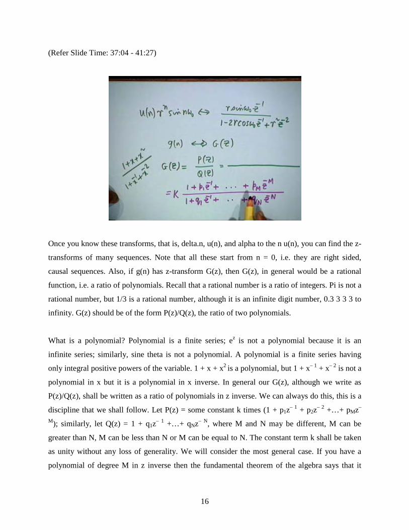
Once you know these transforms, that is, delta.n, u(n), and alpha to the n u(n), you can find the z-

transforms of many sequences. Note that all these start from n = 0, i.e. they are right sided,

causal sequences. Also, if g(n) has z-transform G(z), then G(z), in general would be a rational

function, i.e. a ratio of polynomials. Recall that a rational number is a ratio of integers. Pi is not a

rational number, but 1/3 is a rational number, although it is an infinite digit number, 0.3 3 3 3 to

infinity. G(z) should be of the form P(z)/Q(z), the ratio of two polynomials.

What is a polynomial? Polynomial is a finite series; ez is not a polynomial because it is an

infinite series; similarly, sine theta is not a polynomial. A polynomial is a finite series having

only integral positive powers of the variable. 1 + x + x2 is a polynomial, but 1 + x– 1 + x– 2 is not a

polynomial in x but it is a polynomial in x inverse. In general our G(z), although we write as

P(z)/Q(z), shall be written as a ratio of polynomials in z inverse. We can always do this, this is a

discipline that we shall follow. Let P(z) = some constant k times (1 + p1z– 1 + p2z– 2 +…+ pMz–

M); similarly, let Q(z) = 1 + q1z– 1 +…+ qNz– N, where M and N may be different, M can be

greater than N, M can be less than N or M can be equal to N. The constant term k shall be taken

as unity without any loss of generality. We will consider the most general case. If you have a

polynomial of degree M in z inverse then the fundamental theorem of the algebra says that it

16

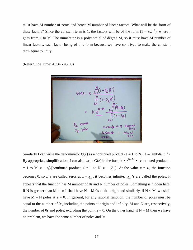
must have M number of zeros and hence M number of linear factors. What will be the form of

these factors? Since the constant term is 1, the factors will be of the form (1 – ziz– 1), where i

goes from 1 to M. The numerator is a polynomial of degree M, so it must have M number of

linear factors, each factor being of this form because we have contrived to make the constant

term equal to unity.


Similarly I can write the denominator Q(z) as a continued product (ℓ = 1 to N) (1 – lambdal z– 1).

By appropriate simplification, I can also write G(z) in the form k × zN– M × [continued product, i

= 1 to M, z – zi]/[continued product, ℓ = 1 to N, z – 1λ ]. At the value z = zi, the function

becomes 0, so zi’s are called zeros at z =1λ , it becomes infinite.

1λ ’s are called the poles. It

appears that the function has M number of 0s and N number of poles. Something is hidden here.

If N is greater than M then I shall have N – M 0s at the origin and similarly, if N < M, we shall

have M – N poles at z = 0. In general, for any rational function, the number of poles must be

equal to the number of 0s, including the points at origin and infinity. M and N are, respectively,

the number of 0s and poles, excluding the point z = 0. On the other hand, if N = M then we have

no problem, we have the same number of poles and 0s.

17


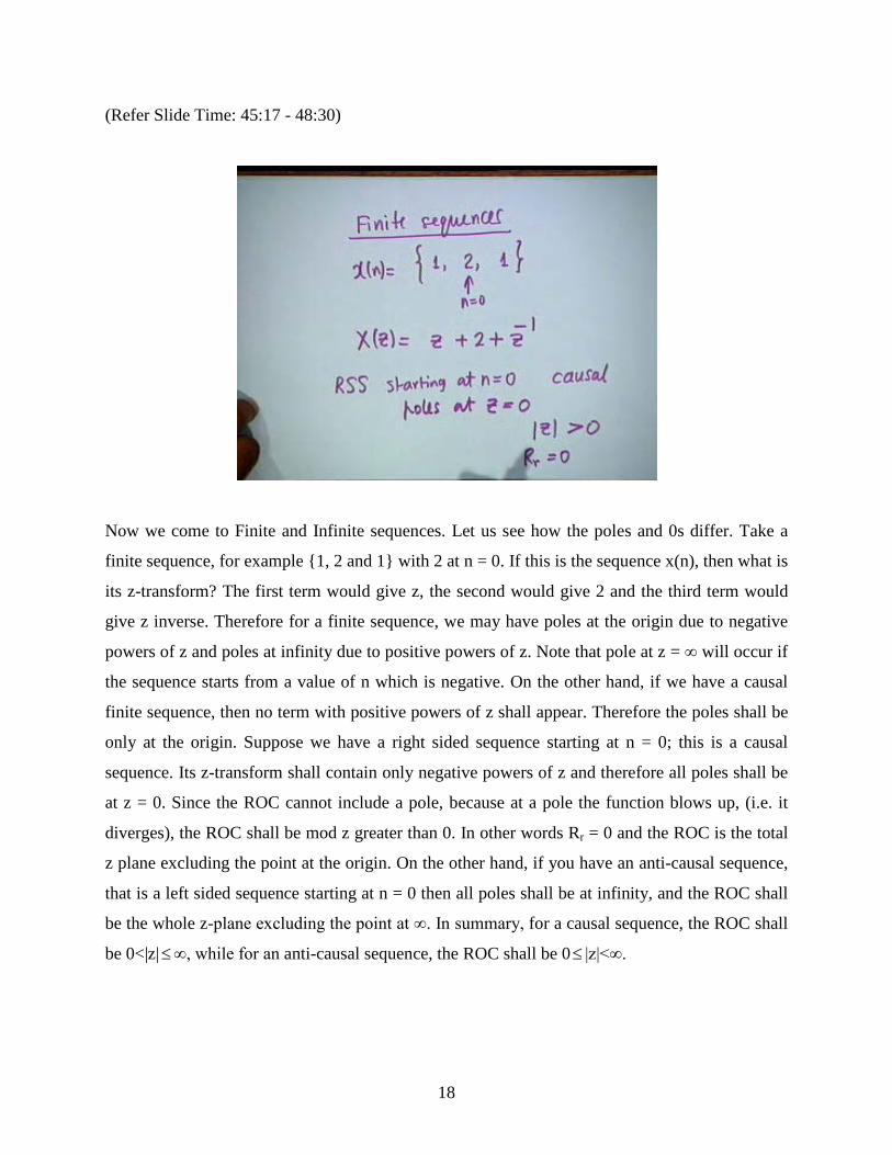
Now we come to Finite and Infinite sequences. Let us see how the poles and 0s differ. Take a

finite sequence, for example {1, 2 and 1} with 2 at n = 0. If this is the sequence x(n), then what is

its z-transform? The first term would give z, the second would give 2 and the third term would

give z inverse. Therefore for a finite sequence, we may have poles at the origin due to negative

powers of z and poles at infinity due to positive powers of z. Note that pole at z = ∞ will occur if

the sequence starts from a value of n which is negative. On the other hand, if we have a causal

finite sequence, then no term with positive powers of z shall appear. Therefore the poles shall be

only at the origin. Suppose we have a right sided sequence starting at n = 0; this is a causal

sequence. Its z-transform shall contain only negative powers of z and therefore all poles shall be

at z = 0. Since the ROC cannot include a pole, because at a pole the function blows up, (i.e. it

diverges), the ROC shall be mod z greater than 0. In other words Rr = 0 and the ROC is the total

z plane excluding the point at the origin. On the other hand, if you have an anti-causal sequence,

that is a left sided sequence starting at n = 0 then all poles shall be at infinity, and the ROC shall

be the whole z-plane excluding the point at ∞. In summary, for a causal sequence, the ROC shall

be 0<|z|≤∞, while for an anti-causal sequence, the ROC shall be 0≤ |z|<∞.

18


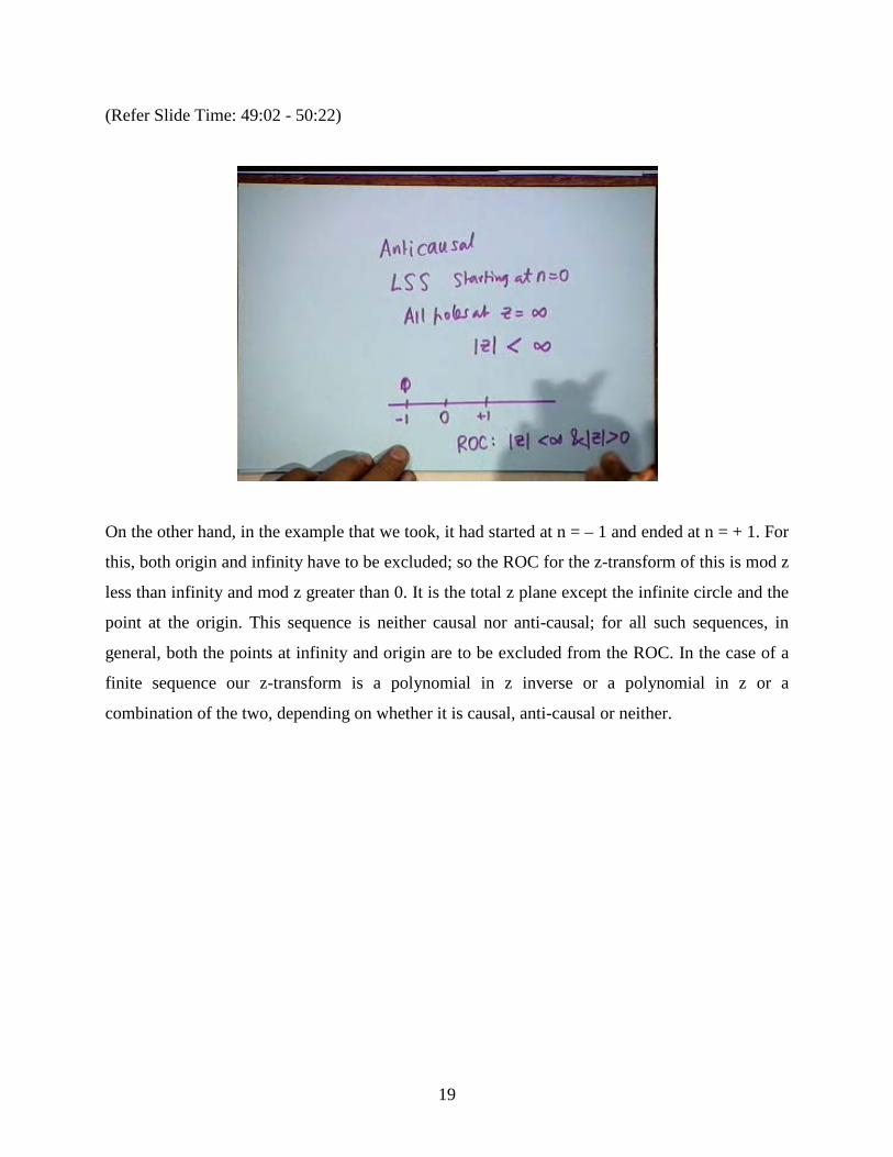
On the other hand, in the example that we took, it had started at n = – 1 and ended at n = + 1. For

this, both origin and infinity have to be excluded; so the ROC for the z-transform of this is mod z

less than infinity and mod z greater than 0. It is the total z plane except the infinite circle and the

point at the origin. This sequence is neither causal nor anti-causal; for all such sequences, in

general, both the points at infinity and origin are to be excluded from the ROC. In the case of a

finite sequence our z-transform is a polynomial in z inverse or a polynomial in z or a

combination of the two, depending on whether it is causal, anti-causal or neither.

19


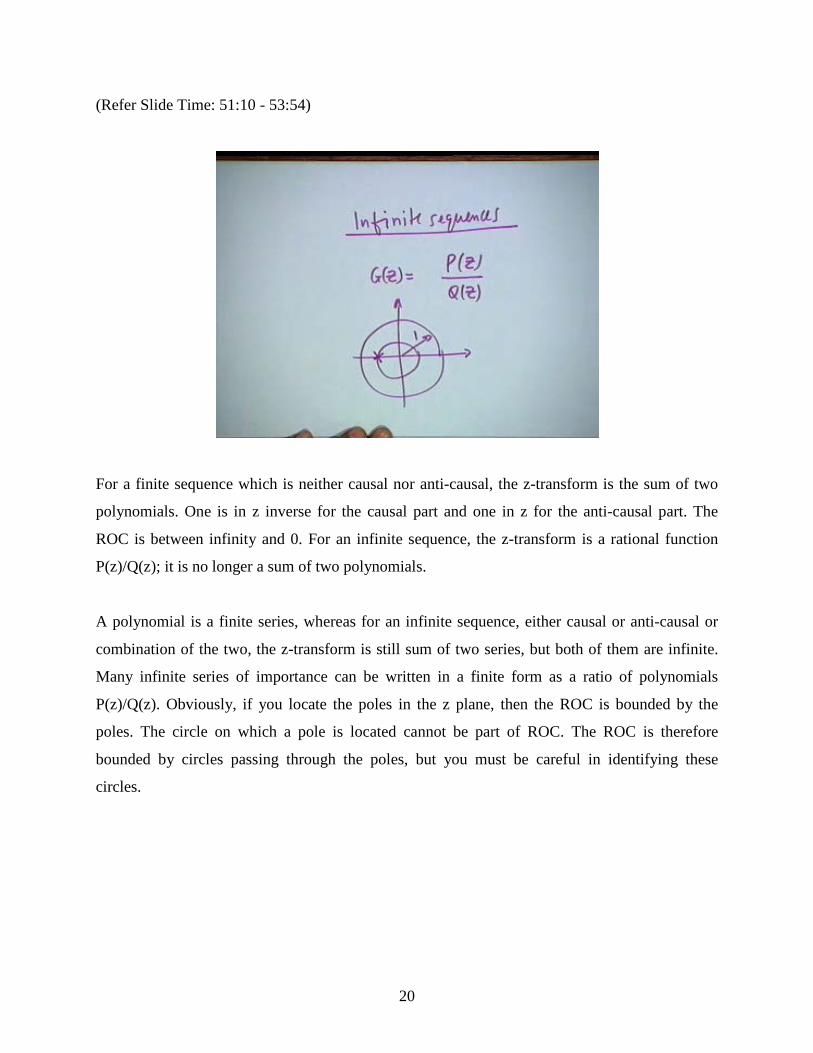
For a finite sequence which is neither causal nor anti-causal, the z-transform is the sum of two

polynomials. One is in z inverse for the causal part and one in z for the anti-causal part. The

ROC is between infinity and 0. For an infinite sequence, the z-transform is a rational function

P(z)/Q(z); it is no longer a sum of two polynomials.

A polynomial is a finite series, whereas for an infinite sequence, either causal or anti-causal or

combination of the two, the z-transform is still sum of two series, but both of them are infinite.

Many infinite series of importance can be written in a finite form as a ratio of polynomials

P(z)/Q(z). Obviously, if you locate the poles in the z plane, then the ROC is bounded by the

poles. The circle on which a pole is located cannot be part of ROC. The ROC is therefore

bounded by circles passing through the poles, but you must be careful in identifying these

circles.

20


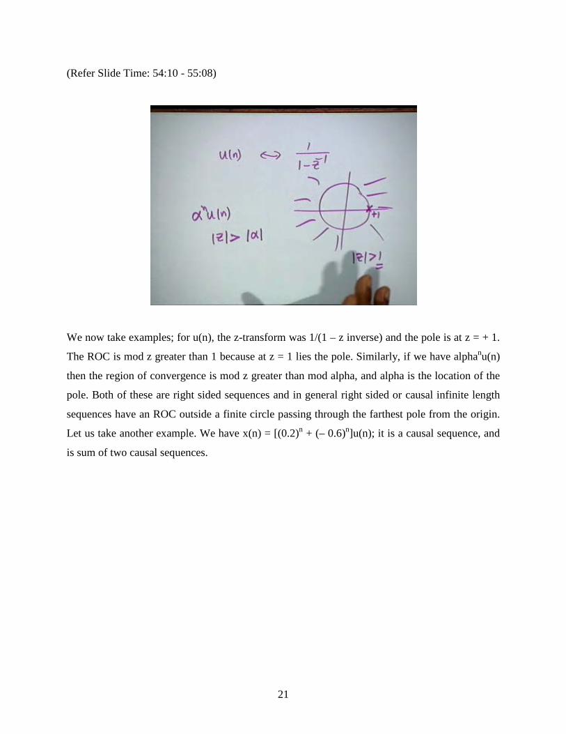
We now take examples; for u(n), the z-transform was 1/(1 – z inverse) and the pole is at z = + 1.

The ROC is mod z greater than 1 because at z = 1 lies the pole. Similarly, if we have alphanu(n)

then the region of convergence is mod z greater than mod alpha, and alpha is the location of the

pole. Both of these are right sided sequences and in general right sided or causal infinite length

sequences have an ROC outside a finite circle passing through the farthest pole from the origin.

Let us take another example. We have x(n) = [(0.2)n + (– 0.6)n]u(n); it is a causal sequence, and

is sum of two causal sequences.

21


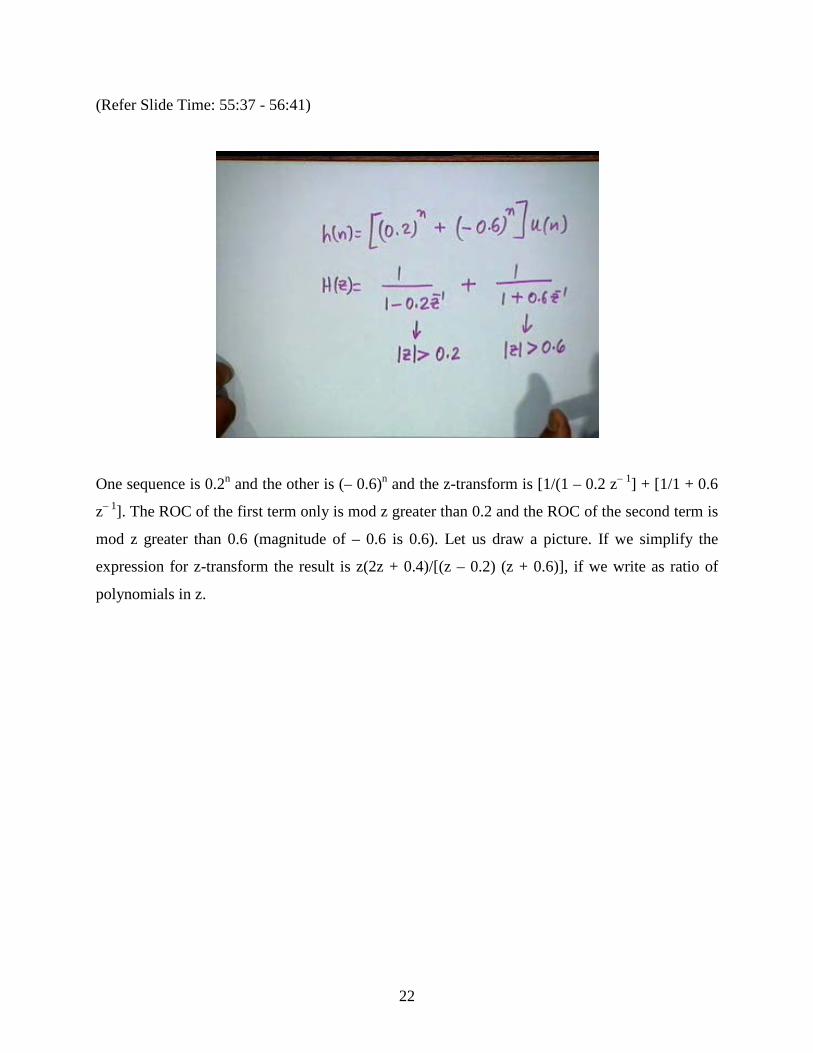
One sequence is 0.2n and the other is (– 0.6)n and the z-transform is [1/(1 – 0.2 z– 1] + [1/1 + 0.6

z– 1]. The ROC of the first term only is mod z greater than 0.2 and the ROC of the second term is

mod z greater than 0.6 (magnitude of – 0.6 is 0.6). Let us draw a picture. If we simplify the

expression for z-transform the result is z(2z + 0.4)/[(z – 0.2) (z + 0.6)], if we write as ratio of

polynomials in z.

22


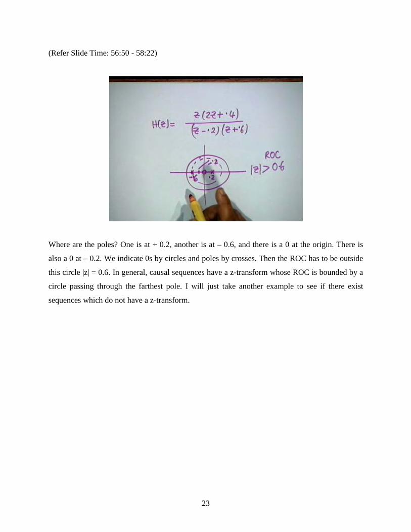
Where are the poles? One is at + 0.2, another is at – 0.6, and there is a 0 at the origin. There is

also a 0 at – 0.2. We indicate 0s by circles and poles by crosses. Then the ROC has to be outside

this circle |z| = 0.6. In general, causal sequences have a z-transform whose ROC is bounded by a

circle passing through the farthest pole. I will just take another example to see if there exist

sequences which do not have a z-transform.

23

(Refer Slide Time: 58:39 - 01:00:53)

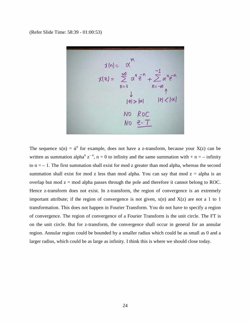
The sequence x(n) = άn for example, does not have a z-transform, because your X(z) can be

written as summation alphan z– n, n = 0 to infinity and the same summation with + n = – infinity

to n = – 1. The first summation shall exist for mod z greater than mod alpha, whereas the second

summation shall exist for mod z less than mod alpha. You can say that mod z = alpha is an

overlap but mod z = mod alpha passes through the pole and therefore it cannot belong to ROC.

Hence z-transform does not exist. In z-transform, the region of convergence is an extremely

important attribute; if the region of convergence is not given, x(n) and X(z) are not a 1 to 1

transformation. This does not happen in Fourier Transform. You do not have to specify a region

of convergence. The region of convergence of a Fourier Transform is the unit circle. The FT is

on the unit circle. But for z-transform, the convergence shall occur in general for an annular

region. Annular region could be bounded by a smaller radius which could be as small as 0 and a

larger radius, which could be as large as infinity. I think this is where we should close today.

24

Documents

Lecture – 11 - NPTELtextofvideo.nptel.ac.in/117102060/lec11.pdf · Lecture - 11 . Discrete Fourier Transform (DFT Cont.) ... How to calculate linear convolution if the two sequences