Lecture 11

FK5024: Particle and Nuclear Physics,Astrophysics and Cosmology

PART III: Astrophysics and CosmologyJon E. Gudmundsson1

jon@fysik.su.se

The third part of this course is meant to provide a very brief introduction to basicastrophysics and cosmology. The coursebook for this part is Andrew R. Liddle’s AnIntroduction to Cosmology (3rd edition), although the first lecture also referencesmaterial in Martin’s Nuclear and particle physics (2nd edition).2 The lecture noteswill cover the topics that are most important for this course. These lecture notesare largely based on the notes passed on from Prof. Lars Bergstrom and Prof. JanConrad who taught this class in 2018. Also, a signification fraction of the belowlecture notes represent abbreviated versions of the textbook discussion.

This lecture should to be complemented by M2.1-M2.3, M8.1, M8.2, M9.1.4(only the neutrino astrophysics part), and chapter 12 of Liddle (L12). Notethat M2.3, M8.1, M8.2, and M9.1.4 in version 2 of Martin’s textbook cor-respond to M2.1-M2.3, M9.1, M9.2, and M10.5.1 (only the neutrino astro-physics part) in the 3rd version of the textbook. Also note that for chaptersM2.1-M2.3, the topics that are reviewed in these lecture are included.

1 Short (and simplified) introduction

The standard cosmological model assumes a Big Bang (some kind of beginning)and a mechanism that facilitates rapid expansion and cooling of space followedby basic element production (hydrogen and helium). Random over-densities in aprimordial matter distribution cause gravitational in-fall and matter accumulationin certain locations of space that eventually leads to star formation. Some of thesestars are short-lived (the massive ones) and eventually die in a supernova explosion.

1http://jon.fysik.su.se2A 3rd edition of Martin’s textbook exists, but we are basing our lectures on the 2nd edition. For those that only

have access to 3rd edition, please reach out to me if you can’t find the equivalent sections in your book.

FK5024 Lecture 11

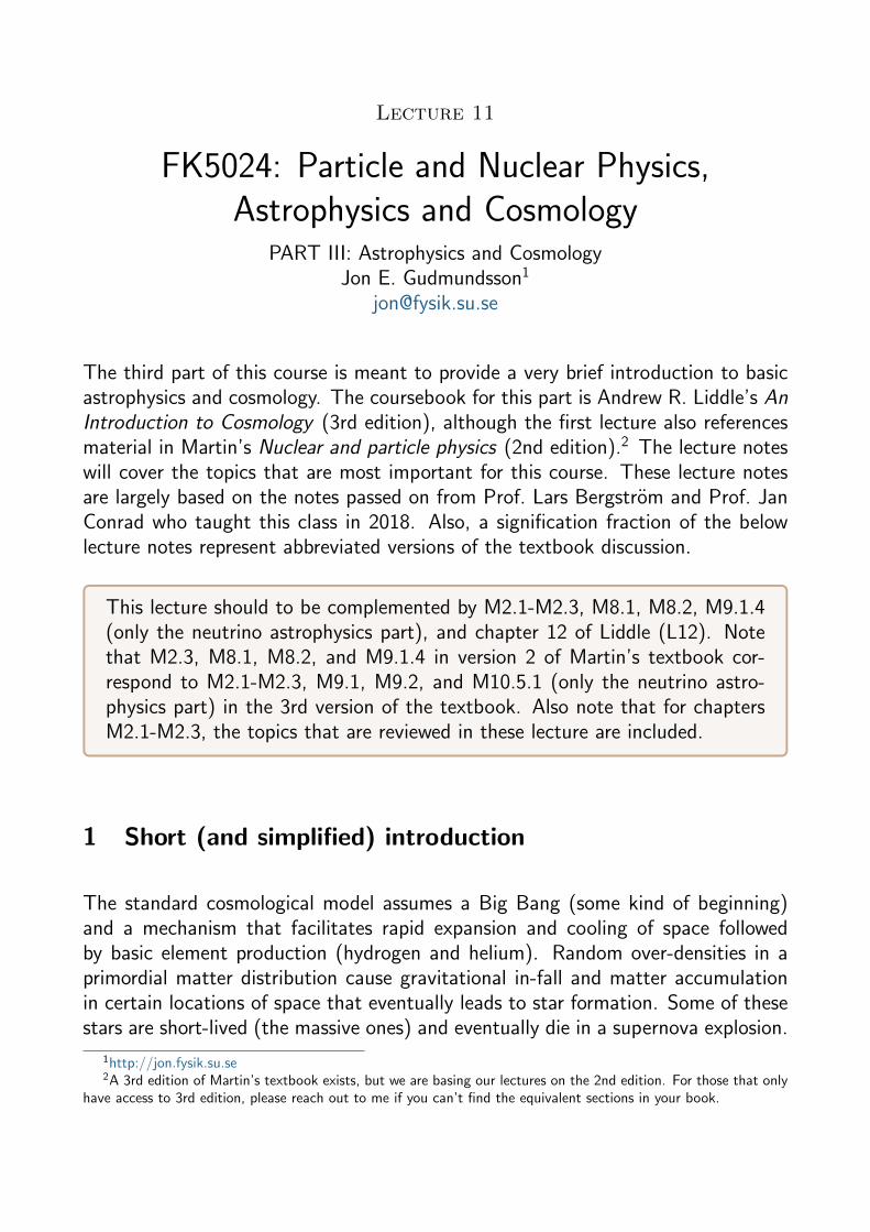
Figure 1: The abundance of elements in the sun plotted as a function of atomic number. Upperlimits denoted with a ’V’. Figure taken from Observation and Analysis of Stellar Photospheres byDavid F. Gray [1].

These explosions are responsible for expelling heavy nuclear elements that are a keyingredient for things like rocky planets and the evolution of life.

2 The stars and our sun

There are ways (absorption spectrometry) to measure the chemical compositionof the sun. Figure 1 shows how such measurements can be used to estimate thefractional abundance of elements in the sun. Things to note:

• Clearly hydrogen and helium make up most of the sun’s mass

• Note the lack of lithium, beryllium, and boron

• The abundance of elements appears to follow an alternating pattern

• There is a gradual decline in abundances as we move to heavier elements

It is particularly important that we understand the origin this odd-even pattern (theOtto-Harkins rule).

2

FK5024 Lecture 11

Note. At this point it might be useful to review the semi-empirical massformula (SEMF). This material is covered in Lectures 6, 7, and 8.

3 Quick thermodynamics recap

A collection of point particles in thermal equilibrium at some temperature T will havean average kinetic energy that is proportional to the temperature. The constantthat relates the gas temperature to the kinetic energy is known as the Boltmannconstant kB = 1.381× 10−23 J/K = 8.617× 10−5 eV/K. The relation is:

3

2kBT =

1

2mv2. (1)

Point particles can have velocity components along three independent (mutuallyorthogonal) directions; they have three degrees of freedom. The average energyper degree of freedom is 1

2kBT .

Note. For those that are interested, the derivation for a Maxwell-Boltzmannvelocity distribution is incredibly clear and easy to follow. With the equationsthat govern likelihood of a certain velocity given a mass and a temperature,you can calculate the likelihood of a finding a particle above a certain velocity.

4 The Coulomb barrier

The Coulomb barrier is the energy required to bring two nuclei close enough togetherto undergo a nuclear reaction (to fuse). Figure 2 shows the binding energy as afunction of atomic mass number, A.

VC =1

4πε0

ZZ ′e2

R +R′

=

(e2

4πε0hc

)hcZZ ′

1.2[A1/3 + (A′)1/3] fm

= 1.198ZZ ′

A1/3 + (A′)1/3MeV (2)

We can for example assume that A ≈ A′ ≈ 2Z ≈ 2Z ′ and get

VC ≈ 0.15A5/3 MeV. (3)

3

FK5024 Lecture 11

Figure 2: Binding energy per nucleon as a function of mass number A for stable and long-livednuclei. See Figure 2.2 in Martin’s textbook.

If we assume that A ≈ 8 (beryllium) we get VC ≈ 4.8 MeV. This is the energythat has to be supplied, for example via kinetic energy, to overcome the Coulombbarrier. It turns out, however, that it is difficult to supply this amount of energyby simply colliding streams of nuclei together at high velocities. Instead, the trickis to provide the conditions for overcoming by this barrier via thermal energy; byheating a collection of nuclei. We can do a rough estimate by using standardthermodynamics relation

E ' kT, (4)

where k is the Boltzmann constant, given by kB = 8.6×10−5eVK−1. Unfortunately,for this to be realistic we would need to raise the temperature of our nuclear matterup to approximately 1011 K. For comparison, the temperature at the core of thesun is thought to be about 2× 106 K. This is obviously not enough.

How is it then that we can have nuclear fusion inside stars? Part of the solutionis the following: A thermalized soup of nuclei will have a (relatively) small numberof nuclei that deviate significantly from the mean of the energy distribution. Theseenergetic nuclei pairs will have enough energy to fuse and create a bound system.

The other part of the solution is related to quantum tunneling (see extended dis-cussion in M.7 and M8.2).

4

FK5024 Lecture 11

5 Stellar fusion [M. 8.2.2]

The stars in the universe are powered by the fusion of hydrogen atoms to formhelium along with heat as byproduct. In the case of our sun, the most significantprocess is known as the proton-proton cycle.

5.1 Proton-proton cycle

There are difference variations of this process, but the following is dominant. Theprocess roughly goes as follows:

The first step is the fusion of two hydrogen nuclei to produce deuterium via theweak interaction:

1H + 1H→ 2H + e+ + νe + 0.42 MeV (5)

Since this is a weak interaction it proceeds at a relatively slow rate.3 The deuteriumthen combines with another hydrogen nucleus to produce 3He:

1H + 2H→ 3He + γ + 5.49 MeV. (6)

Finally, two deuterium nuclei combine to form hydrogen and leftover helium nucleialong with heat.

3He + 3He→ 4He + 2(1H) + 12.86 MeV. (7)

The amount of heat that is released through this process is large because the heliumnucleus is very tightly bound (doubly magical). If we combine all of these processestogether we are left with the following:

4(1H)→ 4He + 2e+ + 2νe + 2γ + 24.68 MeV. (8)

The positrons produced in this process are then annihilated in a collisions withelectrons to release 2×511keV. If we account for kinetic energy loss from neutrinos(about 0.26 MeV on average per neutrino), the total energy released in the proton-proton cycle amounts to about 26.72 MeV.

It is important to note that the temperature in the sun’s core, where this processis taking place, is TCore ≈ 107 K. At these temperatures all material is fully ionized(plasma).

3This sets the scale for the long lifetime of the Sun.

5

FK5024 Lecture 11

Figure 3: Left: The proton-proton cycle. Right: The CNO cycle. Figures from Wikipedia.4

5.2 CNO chain

The carbon, or the CNO chain is an important process in many stellar objects. Itwas once thought that the CNO chain was the primary source of energy, but it hasbeen now shown that it corresponds to only about 3% of the total energy outputof the sun. For more massive stars, the CNO cycle is actually the primary sourceof energy.

12C + 1H→ 13N + γ + 1.95 MeV13N→ 13C + e+ + νe + 1.20 MeV (9)

13C + 1H→ 14N + γ + 7.55 MeV (10)

14N + 1H→ 15O + γ + 7.34 MeV15O→ 15N + e+ + νe + 1.68 MeV (11)

Finally,15N + 1H→ 12C +4 He + 4.96 MeV (12)

The net result of this process is therefore

4(1H)→ 4He + 2e+ + 2νe + 3γ + 24.68 MeV. (13)

4See https://en.wikipedia.org/wiki/CNO cycle

6

FK5024 Lecture 11

Question: What happens when the sun runs of out hydrogen? How does heliumburn?

5.3 Age of the sun

Assuming that the sun luminosity is L� = 3.8× 1026 W. We can estimate that

dNp

dt= L�/6.5 MeV ≈ 3.6× 1038 s−1 (14)

The sun’s mass is approximately M� = 1.99× 1030 kg and about 75% of the sun’smass is in the form of hydrogen. This suggests that Np ≈ 8.9 × 1056. It shouldtherefore take the sun about

Np/(dNp/dt) ≈ 2.4× 1018 s ≈ 8× 1010 years (15)

to convert all of its hydrogen into helium. A more accurate estimate suggests thatour sun should live for about 10 billion years (1010).

6 White dwarfs, neutron stars, and supernovae

This section expands on discussion found in Section 9.1.4 in Martin’s textbook

Main sequence stars owe their name to the fact that their luminosity vs color relationfollows a distinct curve. This group of stars incorporates the majority of stars inthe universe, including our sun.

White dwarfs and neutron stars represent two end-stages for main sequence stars.White dwarfs are held together by electron degeneracy pressure whereas neutronstars are supported by neutron degeneracy pressure. Neutron stars are the mostdense known stellar objects, with the exception of black holes. Their formation isaccompanied with a supernova explosion event which includes a process wherebyelectrons and protons are squashed together to form neutrons. The Pauli exclusionprinciple forces these neutrons to occupy different quantum states and thereforeacts like a pressure term that resists further contraction.

White dwarfs are thought to represent the final evolutionary state of the majorityof main sequence stars, including that of our sun.

7

FK5024 Lecture 11

6.1 White dwarfs and Pauli’s exclusion principle (optional)

It is interesting to look at the approximate equations governing the radius of whitedwarfs. The Heisenberg uncertainty principle states that

∆x∆p ≥ h. (16)

Under immense pressures, each electron is forced to stay within a volume V ∼ n−1e .We can therefore assume that the location of each electron is known to within ∆x ∼V 1/3 ∼ n

−1/3e . The uncertainty in the electron momentum is therefore

∆p ∼ h

∆x∼ hn1/3e . (17)

Assuming that the electrons are nonrelativistic, we can write

∆v =∆p

me∼ hn

1/3e

me. (18)

Thanks to the Heisenberg uncertainty principle, the electrons in a tightly packed

object are moving at speeds ve ∝ n1/3e and this relation is independent of temper-

ature. We know from thermodynamics, that for a standard thermal picture, theelectrons are moving at speeds

vth ∼(kT

me

)1/2

, (19)

and similarly, the pressure from the thermal motion of these electrons is

Pth = nekT ∼ nemev2th. (20)

By analogy, the ”Heisenberg speeds” contribute a degeneracy pressure

Pdegen ∼ neme(∆v)2 ∼ neme

(hn

1/3e

me

)2

∼ h2n5/3e

me(21)

For any object in hydrostatic equilibrium, the pressure at the center is

Pc ∼GM 2

R4. (22)

Assuming this pressure is provided by electron degeneracy pressure, we find that

Pc ∼ h2n5/3e

me∼ h2 ρ5/3

m5/3p me

∼ h2

m5/3p me

M 5/3

R5(23)

8

FK5024 Lecture 11

Combining this last result with Eqation 22 we find that

GM 2

R4∼ h2

m5/3p me

M 5/3

R5(24)

which gives

R ∼ h2

Gmem2p

(M

mp

)−1/3. (25)

Somewhat surprisingly, the size of a white dwarf goes down as you increase its mass.Obviously, the above derivation made many simplifying assumptions, but the roughresult is still valid. The more accurate derivation was Chandrasekhar and others.Stars at the end of their life whose mass exceeds the Chandrasekhar limit evolve tobecome neutron stars.

6.2 Neutron stars

If the mass of a star exceeds the Chandrasekhar limit, M > 1.4M�, it will evolveto become a neutron star. In the case of very massive stars, the run of events canlook something like the following:

1. Stars with mass greater than about 11 solar masses (M�) can evolve throughall stages of fusion ending in a core of iron surrounded by shells of lighterelements

2. Thermonuclear fusion of iron is not possible and therefore the core will contractunder gravity

3. Initially this process is resisted by electron degeneracy pressure, but if themass of the core exceeds M = 1.4M� (the Chandrasekhar limit) the electronsare unable to support the core and a collapse within an explosion becomesinevitable

4. We subsequently have photodisintegration of iron and other nuclei followedphotodisintegration of helium into protons and neutrons

The photodisintegration of iron can be described by,

γ + 56Fe→ 13(4He) + 4n, (26)

followed by further splitting of the helium nuclei into protons and neutrons.

γ + 4He→ 2p+ 2n. (27)

9

FK5024 Lecture 11

Figure 4: A table of elements with color coding corresponding to the mechanism responsible for theelement abundance. Figure created by Jennifer Johnson (from A Chemical History of the Universe).Note that this figure is effectively being updated constantly as new data are gathered.

As this process continues, eventually the electrons have enough energy to faciliatea weak interaction whereby electrons and protons fuse to form neutrons

e− + p→ n+ νe. (28)

The gravitational collapse stops abruptly when the neutron degeneracy pressurecounters the gravitational pressure. This generates a core-collapse shock wave thatexpels matter, radiation, and neutrinos.

It turns out, that the majority (99%) of energy radiated away from a core-collapsesupernova is in the form of neutrinos because of their low scattering cross section.When all of this is done, most of the mass of the star is in the form of neutrons.

A typical neutron star could have the following properties:

• Mass: M ≈ 1.5M�

• Radius: R ≈ 10 km

• Density: ρ ≈ 1014 g/cm3

Note. A lot is still unknown about the physics that are in play during theformation of a neutron stars and there are lot of active research groupsworking on generating more accurate numerical simulations of events leading

10

FK5024 Lecture 11

up to the formation of a neutron star. One group is lead by Stephan Rosswoghere at Stockholm University.

6.3 Supernovae

A sufficiently massive star will end its life cycle in an explosion referred to as asupernova event. There are different types of supernovae and these are characterizedby the time evolution of their spectrum and the events leading up to the explosion.Some supernovae happen when white dwarfs are reignited by the accumulation ofmatter, for example from a binary companion. Others simply happen when a verymassive star ends it life (see description in 6.2).

It is estimated that roughly 1-3 stars in our own Galaxy end with supernovae ex-plosions per century. We only see a fraction of those because occlusion from otherstellar objects in our Galaxy.

A particularly useful group of supernovae are known as type Ia supernovae. Thesetypes of supernovae are generated when a white dwarf is reignited by the accumu-lation of matter, typically from a companion star. Because of the mass limit forelectron degeneracy pressure to be able to prevent further gravitational collapse isfixed, roughly M = 1.4M�, the critical mass is fixed and therefore the peak lumi-nosity of the explosion is quite consistent between events. This suggests that thetype Ia supernovae can serve as standard candles throughout the universe. We willdiscuss that further in subsequent lectures.

7 Kamiokande, Amanda, and IceCube (Optional)

Famously, the Kamiokande and IMB experiments measured a stream of neutrinosin their water Cherenkov detectors in 1987.5 This signal was then used to constrainthe mass of the neutrinos (see discussion in Liddle 9.1.4). The 2002 Nobel prizein physics was in part awarded for the work leading to the detection of cosmicneutrinos.

We estimate roughly 1-3 supernova events per century in our galaxy. We expectthat such a supernova event will register in experiments like Super-Kamiokande(see Figure 5). Within seconds of this happening, such experimental collaborationshope to be able to send alarms to other astrophysical observatories. The data

5These neutrinos are thought to have come from SN1987A

11

FK5024 Lecture 11

Figure 5: Super-Kamiokande experiment is an underground detector filled with ultra-pure water(50,000 tons) that is surrounded by photomultiplier tubes. The detector is placed 1km undergroundto shield from unwanted radiation signal.

from modern-day observations of a nearby supernova would likely revolutionize ourunderstanding of various physical processes. The 2015 Nobel prize in physics wasawarded in recognition of Super-Kamiokande measurements of neutrino oscillations.

The IceCube Neutrino Observatory is a large scientific experiment placed at theSouth Pole. It uses thousands of photomultiplier tubes mounted on vertical stringsthat penetrate km-deep boreholes in the Antarctica ice sheet. The idea is that high-energy neutrinos will occasionally interact with water molecules in the ice creatinga stream of charged particles that emit Cherenkov radiation. The predecessor tothe IceCube experiment was the Amanda experiment.

Note. The IceCube experiment has significant contributions from StockholmUniversity. If you are interested in the science that they do, you should reachout to people like Chad Finley and Klas Hultqvist.a

aSee https://www.su.se/profiles/klas-1.186617 and https://www.su.se/profiles/cfinl-1.187008

8 Black holes

If the mass of a stellar object becomes sufficiently large, even the neutron degeneracypressure will not be able to resist gravitational collapse. The star becomes a blackhole.

12

FK5024 Lecture 11

9 Big bang nucleosynthesis

Big bang nucleosynthesis (BBN) is a concept that is commonly brought up in bothastrophysical and cosmological context. It describes the physics of element pro-duction during the early stages in the history of our universe. For those who areinterested, Steven Weinberg wrote a famous book called The First Three Min-utes [2].

Chapter 12 in Liddle discusses light element production, in particular hydrogen andhelium, during the first few minutes in the history of our big bang cosmologicalmodel. Some concepts to take away from this chapter include:

• BBN is responsible for the production of hydrogen, helium, deuterium, andeven lithium; there is a primordial abundance that we can measure today

• Nucleosynthesis is happening at temperatures corresponding to 1 MeV

• Nucleosynthesis happens during the first few minutes in the history of ouruniverse

• At the end of this process, we are left with approximately 75% hydrogen, and25% helium

• A tiny mass fraction in the form of deuterium, helium-3, and lithium (lithium-6and lithium-7 are both stable)

If we consider a time-period where the universe has cooled sufficiently rapidly so thatprotons and neutrons are non-relativistic, but before nuclei have formed. Assumingprotons and neutrons are non-relativistic and in thermal equilibrium it is safe toassume that they follow the Maxwell-Boltzmann distribution. In that case, thenumber density is given by

N ∝ m3/2 exp

(−mc2

kBT

). (29)

The particles are in thermal equilibrium (at the same temperature) and we cantherefore write

Nn

Np=

(mn

mp

)3//2

exp

[−(mn −mp)c

2

kBT

]. (30)

Since the mass of protons and neutrons are very similar we note that the numberof neutrons and protons will be quite similar in the primordial plasma as long askBT � (mn −mp)c

2.

13

FK5024 Lecture 11

Neutrons and protons are coupled through the following conversion process

n+ νe ←→ p+ e−, (31)

n+ e+ ←→ p+ νe. (32)

As long as these processes continue at a sufficient rate, the two particles remainin thermal equilibrium. We find that the reaction rate is high as long as kBT '0.8 MeV (T ' 1010 K), but eventually this process dies down and the relativenumber density of neutrons versus protons is

Nn

Np' exp

(−1.3 MeV

0.8 MeV

)' 1

5. (33)

References

[1] Gray, D.F. The Observation and Analysis of Stellar Photospheres. Cam-bridge University Press, 3 edition, 2005.

[2] Weinberg, S. The First Three Minutes. Basic Books, New York, NY, 1993.

14