Lecture 11 Fast Fourier Transform (FFT) - Welcome to …dsec.pku.edu.cn/~tieli/notes/num_meth/lect11.pdfExamples Fast Fourier Transform Applications Signal processing I Filtering:

Lecture 11 Fast Fourier Transform (FFT)

Weinan E1,2 and Tiejun Li2

1Department of Mathematics,

Princeton University,

[email protected]

2School of Mathematical Sciences,

Peking University,

[email protected]

No.1 Science Building, 1575

Examples Fast Fourier Transform Applications

Outline

Examples

Fast Fourier Transform

Applications


Signal processing

I Filtering: a polluted signal

0 200 400 600 800 1000 1200−1.5

−1

−0.5

0

0.5

1

1.5

I High pass and low pass filter (signal and noise)

0 200 400 600 800 1000 1200−1.5

−1

−0.5

0

0.5

1

1.5

I How to obtain the high frequency and low frequency quickly?


Solving PDEs on rectangular mesh

I Solving the Poisson equations

−∆u = f in Ω

u = 0 on ∂Ω

in the rectangular domain

I After discretization we will obtain the linear system with about N2

unknowns

−ui+1,j + ui−1,j + ui,j+1 + ui,j−1 − 4ui,j

4h2= fij

I The FFT would give a fast algorithm to solve the system above with

computational efforts O(N2 log2 N).


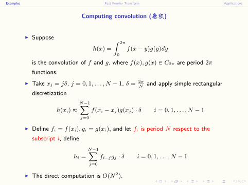
Computing convolution (òòòÈÈÈ)

I Suppose

h(x) =

∫ 2π

0

f(x− y)g(y)dy

is the convolution of f and g, where f(x), g(x) ∈ C2π are period 2π

functions.

I Take xj = jδ, j = 0, 1, . . . , N − 1, δ = 2πN

and apply simple rectangular

discretization

h(xi) ≈N−1∑j=0

f(xi − xj)g(xj) · δ i = 0, 1, . . . , N − 1

I Define fi = f(xi), gi = g(xi), and let fi is period N respect to the

subscript i, define

hi =

N−1∑j=0

fi−jgj · δ i = 0, 1, . . . , N − 1

I The direct computation is O(N2).



Fast Fourier Transform is one of the top 10 algorithms in 20th century.

But its idea is quite simple, even for a high school student!


Outline

Examples


Applications


Fourier Transform

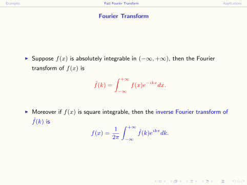
I Suppose f(x) is absolutely integrable in (−∞, +∞), then the Fourier

transform of f(x) is

f(k) =

∫ +∞

−∞f(x)e−ikxdx.

I Moreover if f(x) is square integrable, then the inverse Fourier transform of

f(k) is

f(x) =1

2π

∫ +∞

−∞f(k)eikxdk.


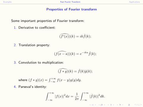
Properties of Fourier transform

Some important properties of Fourier transform:

1. Derivative to coefficient:

(f ′(x))(k) = ikf(k);

2. Translation property:

(f(x− a))(k) = e−ikaf(k);

3. Convolution to multiplication:

(f ∗ g)(k) = f(k)g(k);

where (f ∗ g)(x) =∫ +∞−∞ f(x− y)g(y)dy.

4. Parseval’s identity:∫ +∞

−∞|f(x)|2dx =

1

2π

∫ +∞

−∞|f(k)|2dk.


Discrete Fourier transform (DFT)

I Suppose we have a = (a0, a1, · · · , aN−1)T , define DFT of a as

c = (c0, c1, · · · , cN−1)T ∆

= a, where

ck =

N−1∑j=0

aje−jk 2πi

N , k = 0, 1, . . . , N − 1.

Here i is the imaginary unit, e−2πiN

∆= ω is the N -th root of unity.

I a is the inverse discrete Fourier transform of c defined as

aj =1

N

N−1∑k=0

ckejk 2πiN , j = 0, 1, . . . , N − 1.

I DFT is closely related to the trigonometric interpolation for 2π-periodic

function

T (x) =

N2∑

k=−N2 +1

bkeikx.

such that at xj = 2jπN

, T (xj) = aj , j = 0, 1, . . . , N − 1. The readers

may find the relation between ck and bk.


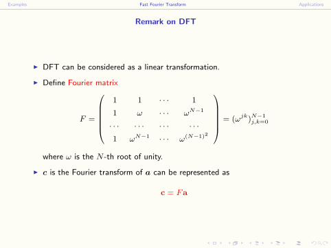
Remark on DFT

I DFT can be considered as a linear transformation.

I Define Fourier matrix

F =

1 1 · · · 1

1 ω · · · ωN−1

· · · · · · · · · · · ·1 ωN−1 · · · ω(N−1)2

= (ωjk)N−1j,k=0

where ω is the N -th root of unity.

I c is the Fourier transform of a can be represented as

c = Fa


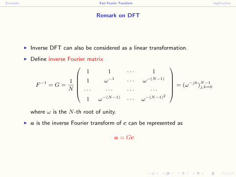
Remark on DFT

I Inverse DFT can also be considered as a linear transformation.

I Define inverse Fourier matrix

F−1 = G =1

N

1 1 · · · 1

1 ω−1 · · · ω−(N−1)

· · · · · · · · · · · ·1 ω−(N−1) · · · ω−(N−1)2

= (ω−jk)N−1j,k=0

where ω is the N -th root of unity.

I a is the inverse Fourier transform of c can be represented as

a = Gc


Properties of DFT

I Convolution to multiplication:

(f ∗ g)k = fkgk k = 0, 1, . . . , N − 1

where

(f ∗ g)l =

N−1∑j=0

fl−jgj l = 0, 1, . . . , N − 1,

and fl is period N with respect to index l, i.e.

f−1 = fN−1, f−2 = fN−2, . . .

I Parseval’s identity:

N

N−1∑j=0

|aj |2 =

N−1∑k=0

|ck|2


FFT idea

I FFT is proposed by J.W. Cooley and J.W. Tukey in 1960s, but the idea

may be traced back to Gauss.

I The basic motivation is if we compute DFT directly, i.e.

c = Fa

we need N2 multiplications and N(N − 1) additions. Is it possible to

reduce the computation effort?

I First consider the case N = 4

F =

1 1 1 1

1 −i −1 i

1 −1 1 −1

1 i −1 −i

, Fa =

(a0 + a2) + (a1 + a3)

(a0 − a2)− i(a1 − a3)

(a0 + a2)− (a1 + a3)

(a0 − a2) + i(a1 − a3)


FFT idea

I From the concrete form of DFT, we actually need 2 multiplications

(timing ±i) and 8 additions (a0 + a2, a1 + a3, a0 − a2, a1 − a3 and the

additions in the middle).

I This observation may reduce the computational effort from O(N2) into

O(N log2 N)

I Because

limN→∞

log2 N

N= 0

It is a typical fast algorithm.

I Fast algorithms of this type of recursive halving are very typical in

scientific computing.


Construction of FFT

I Consider N = 2m and denote

p(x) = a0 + a1x + · · ·+ aN−1xN−1,

divide p(x) into odd (Û) and even (ó) power parts

p(x) = (a0 + a2x2 + · · · ) + x(a1 + a3x

2 + · · · )

= pe(x2) + xpo(x

2)

where

pe(t) = a0 + a2t + . . . + aN−2tN2 −1, po(t) = a1 + a3t + . . . + aN−1t

N2 −1

I Define ωk = e−2πik (k-th root of unity), then when j = 0, 1, . . . , N

2− 1 cj = pe(ω

2jN ) + ωj

Npo(ω2jN )

c N2 +j = pe(ω

2( N2 +j)

N ) + ωN2 +j

N po(ω2( N

2 +j)

N )


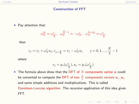
Construction of FFT

I Pay attention that

ω2jN = ωj

N2

, ωN2 +j

N = −ωjN , ωN+2j

N = ωjN2

then

cj = vj + ωjNuj , cj+ N

2= vj − ωj

Nuj j = 0, 1, ...,N

2− 1

where

vj = pe(ωjN2

), uj = po(ωjN2

)

I The formula above show that the DFT of N components vector a could

be converted to compute the DFT of two N2

components vectors ae, ao

and some simple additions and multiplications. This is called

Danielson-Lanczos algorithm. The recursive application of this idea gives

FFT.


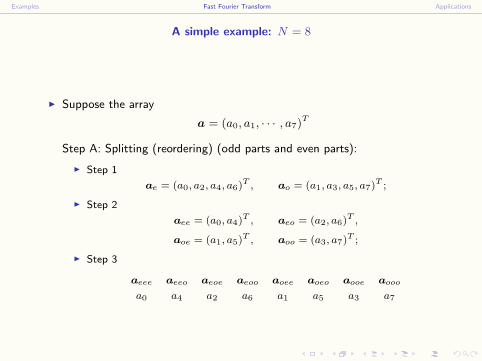
A simple example: N = 8

I Suppose the array

a = (a0, a1, · · · , a7)T

Step A: Splitting (reordering) (odd parts and even parts):

I Step 1

ae = (a0, a2, a4, a6)T , ao = (a1, a3, a5, a7)T ;

I Step 2

aee = (a0, a4)T , aeo = (a2, a6)T ,

aoe = (a1, a5)T , aoo = (a3, a7)T ;

I Step 3

aeee aeeo aeoe aeoo aoee aoeo aooe aooo

a0 a4 a2 a6 a1 a5 a3 a7



Step B: Combination:

I Step 1

cee = (a0 + ω02a4, a0 − ω0

2a4)T,

ceo = (a2 + ω02a6, a2 − ω0

2a6)T,

coe = (a1 + ω02a5, a1 − ω0

2a5)T,

coo = (a3 + ω02a7, a3 − ω0

2a7)T,

I Define the notations

w4 , (w04, w1

4)T , w8 , (w0

8, w18, w2

8, w38)

T ,

and

X Y , (xjyj)j

as the vector product through multiplication by components.



Step B: Combination:

I Step 2

ce =

[cee + w4 ceo

cee −w4 ceo

], co =

[coe + w4 coo

coe −w4 coo

],

I Step 3

c =

[ce + w8 c0

ce −w8 c0

]


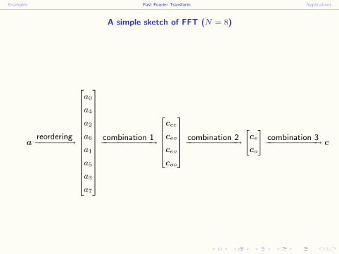
A simple sketch of FFT (N = 8)

areordering−−−−−−−→

a0

a4

a2

a6

a1

a5

a3

a7

combination 1−−−−−−−−−−−→

cee

ceo

ceo

coo

combination 2−−−−−−−−−−−→

[ce

co

]combination 3−−−−−−−−−−−→ c


A remark on the reordering

If we map e to 0, and o to 1§we can find the binary representation of the

indices after reordering is just the bit reversal before reordering

0= 0002

1= 0012

2= 0102

3 = 0112

4 = 1002

5 = 1012

6 = 1102

7 = 1112

Bit reversal−−−−−−−→

0002 = 0

1002 = 4

0102 = 2

1102 = 6

0012 = 1

1012= 5

0112= 3

1112= 7


Outline

Examples


Applications


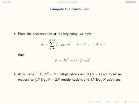
Compute the convolution

I From the discretization at the beginning, we have

hi =

N−1∑j=0

fi−jgj · δ i = 0, 1, . . . , N − 1

thus

h = (h)∨ = (δ · f g)∨

I After using FFT, N2 + N multiplications and N(N − 1) additions are

reduced to 32N log2 N + 2N multiplications and 3N log2 N additions.


Solving the linear system with loop matrix

I Let

L =

c0 cN−1 · · · c1

c1 c0 · · · c2

· · · · · · · · · · · ·cN−1 cN−2 · · · c0

Solving Lx = b. L is a loop matrix.

I We have

(Lx)i =

N−1∑j=0

ci−jxj

where we assume c is period N with respect to the subscripts, and

x = (x0, x1, . . . , xN−1)T .



I First consider the Jordan form of L. From the formula before

Lx = c ∗ x = λx

Take DFT we have

c x = λx

then eigenvalues

λk = ck

I The eigenvectors

x(k)j = δkj , (j, k = 0, 1, . . . , N − 1)

where δkj is Kronecker’s δ.

I Take inverse transform we obtain

x(0) = (1, 1, . . . , 1)T ,

x(1) = (1, ω−1, . . . , ω−(N−1))T ,

. . . . . . . . .

x(N−1) = (1, ω−(N−1), . . . , ω−(N−1)2)T



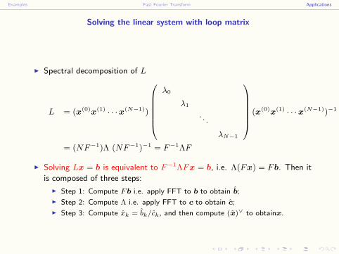
I Spectral decomposition of L

L = (x(0)x(1) · · ·x(N−1))

λ0

λ1

. . .

λN−1

(x(0)x(1) · · ·x(N−1))−1

= (NF−1)Λ (NF−1)−1 = F−1ΛF

I Solving Lx = b is equivalent to F−1ΛFx = b, i.e. Λ(Fx) = Fb. Then it

is composed of three steps:

I Step 1: Compute Fb i.e. apply FFT to b to obtain b;

I Step 2: Compute Λ i.e. apply FFT to c to obtain c;

I Step 3: Compute xk = bk/ck, and then compute (x)∨ to obtainx.


Homework assignment

I Familiarize the “FFT” and “IFFT” command in MATLAB;

I Compute the convolution for

h(x) =

∫ 2π

0

sin(x− y)ecos ydy

Documents

Lecture 11 Fast Fourier Transform (FFT) - Welcome to …dsec.pku.edu.cn/~tieli/notes/num_meth/lect11.pdfExamples Fast Fourier Transform Applications Signal processing I Filtering: