Macroeconomics 1

Lecture 11: ASAD model

Dr Gabriela Grotkowska

slide 2

Lecture objectives

difference between short run & long run

aggregate demand

aggregate supply in the short run & long run

see how model of aggregate supply and demand can be used to analyze short-run and long-run effects of “shocks”

slide 3

-10

-5

0

5

10

15

1960 1965 1970 1975 1980 1985 1990 1995 2000 2005

Perc

en

t ch

an

ge f

rom

pre

vio

us

qu

art

er,

at

an

nu

al

rate

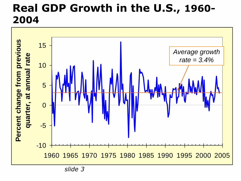
Real GDP Growth in the U.S., 1960-

2004

Average growth

rate = 3.4%

Time horizons

Long run: Prices are flexible, respond to changes in supply or demand

Short run: many prices are “sticky” at some predetermined level

The economy behaves much

differently when prices are sticky.

slide 6

In Classical Macroeconomic Theory

Output is determined by the supply side:

supplies of capital, labor

technology

Changes in demand for goods & services (C, I, G ) only affect prices, not quantities.

Complete price flexibility is a crucial assumption, so classical theory applies in the long run.

slide 7

When prices are sticky

…output and employment also depend

on demand for goods & services,

which is affected by

fiscal policy (G and T )

monetary policy (M )

other factors, like exogenous changes

in C or I.

slide 8

The model of aggregate demand and supply

the paradigm that most mainstream

economists & policymakers use to think

about economic fluctuations and policies

to stabilize the economy

shows how the price level and aggregate

output are determined

shows how the economy’s behavior is

different in the short run and long run

slide 9

Aggregate demand

The aggregate demand curve shows the

relationship between the price level and

the quantity of output demanded.

It may be derived from Quantity Theory

of Money.

It may be developed from Keynesian

Cross.

slide 10

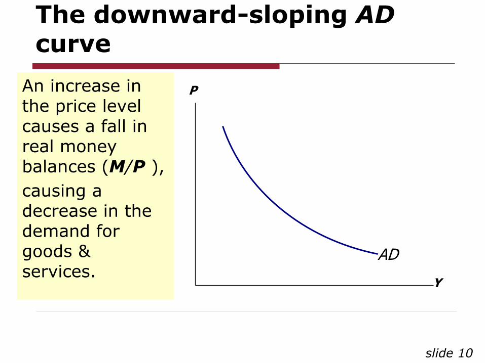
The downward-sloping AD curve

An increase in the price level causes a fall in real money balances (M/P ),

causing a decrease in the demand for goods & services.

Y

P

AD

slide 11

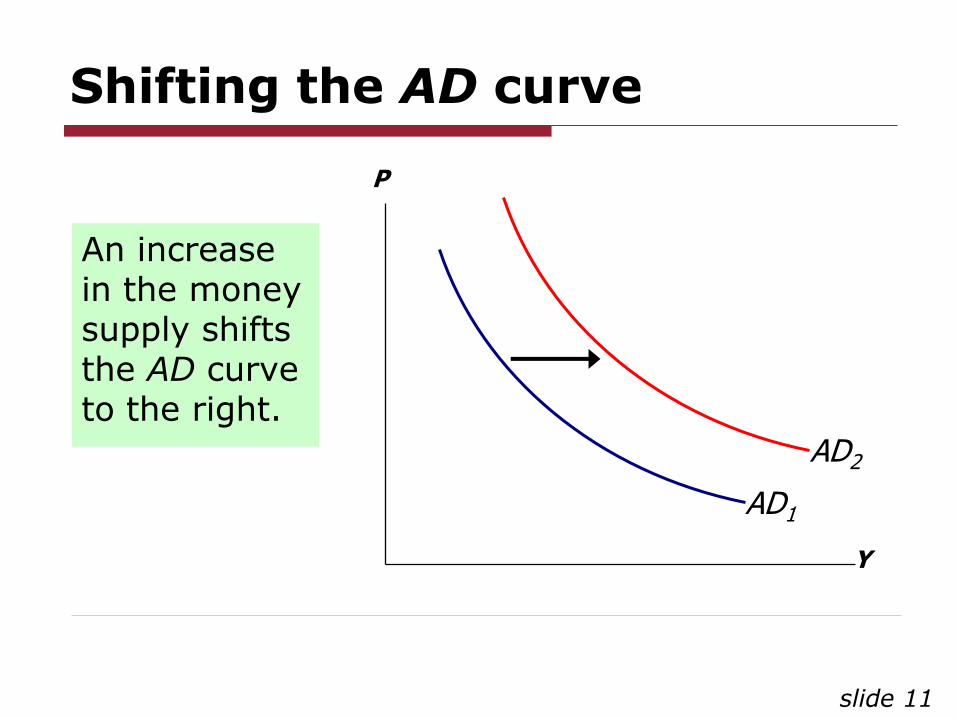
Shifting the AD curve

An increase in the money supply shifts the AD curve to the right.

Y

P

AD1

AD2

slide 12

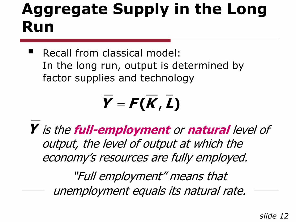
Aggregate Supply in the Long Run

Recall from classical model:

In the long run, output is determined by

factor supplies and technology

, ( )Y F K L

is the full-employment or natural level of output, the level of output at which the economy’s resources are fully employed.

Y

“Full employment” means that unemployment equals its natural rate.

slide 13

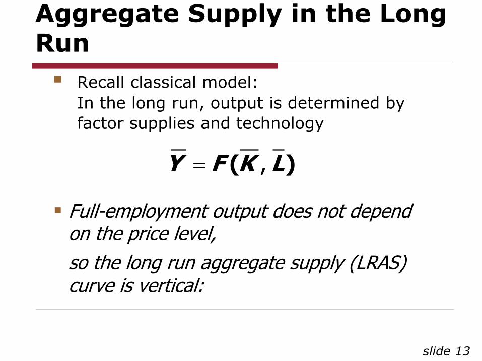
Aggregate Supply in the Long Run

Recall classical model:

In the long run, output is determined by

factor supplies and technology

Full-employment output does not depend on the price level,

so the long run aggregate supply (LRAS) curve is vertical:

, ( )Y F K L

slide 14

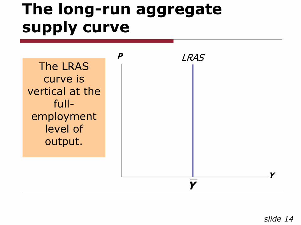
The long-run aggregate supply curve

Y

P LRAS

Y

The LRAS curve is

vertical at the full-

employment level of output.

slide 15

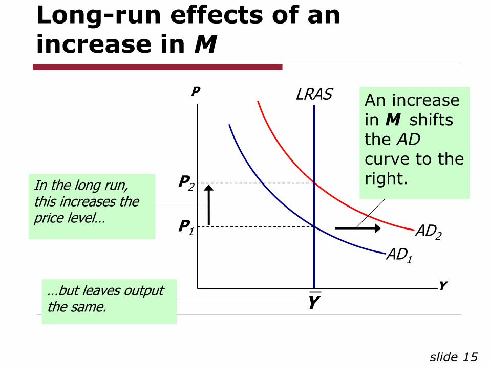
Long-run effects of an increase in M

Y

P

AD1

AD2

LRAS

Y

An increase in M shifts the AD

curve to the right.

P1

P2 In the long run, this increases the price level…

…but leaves output the same.

slide 16

Aggregate Supply in the Short Run

In the real world, many prices are sticky in the short run.

For now, we assume that all prices are stuck at a predetermined level in the short run…

…and that firms are willing to sell as much at that price level as their customers are willing to buy.

Therefore, the short-run aggregate supply (SRAS) curve is horizontal:

slide 17

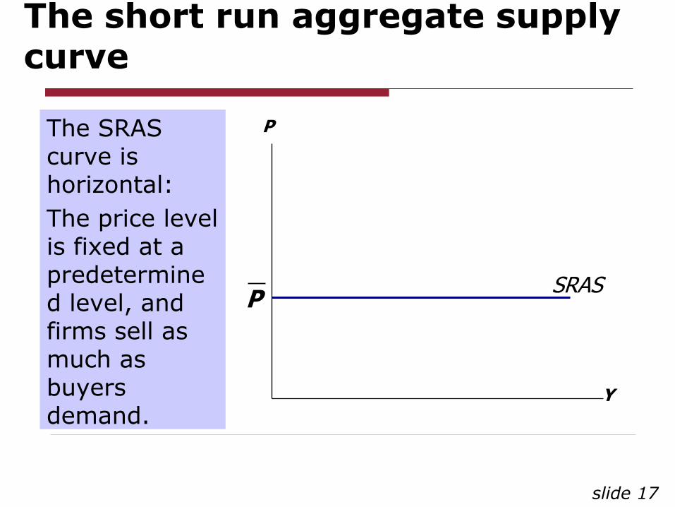
The short run aggregate supply curve

Y

P

PSRAS

The SRAS curve is horizontal:

The price level is fixed at a predetermined level, and firms sell as much as buyers demand.

slide 18

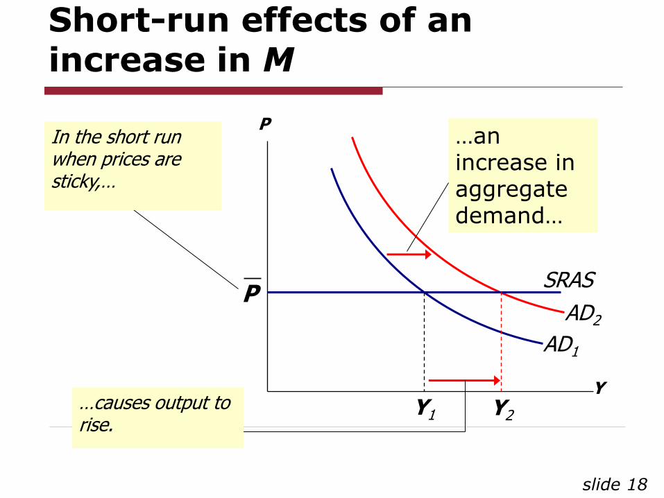
Short-run effects of an increase in M

Y

P

AD1

AD2

…an increase in aggregate demand…

In the short run when prices are sticky,…

…causes output to rise.

PSRAS

Y2 Y1

slide 19

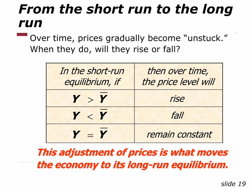
From the short run to the long run

Over time, prices gradually become “unstuck.”

When they do, will they rise or fall?

Y Y

Y Y

Y Y

rise

fall

remain constant

In the short-run equilibrium, if

then over time, the price level will

This adjustment of prices is what moves

the economy to its long-run equilibrium.

slide 20

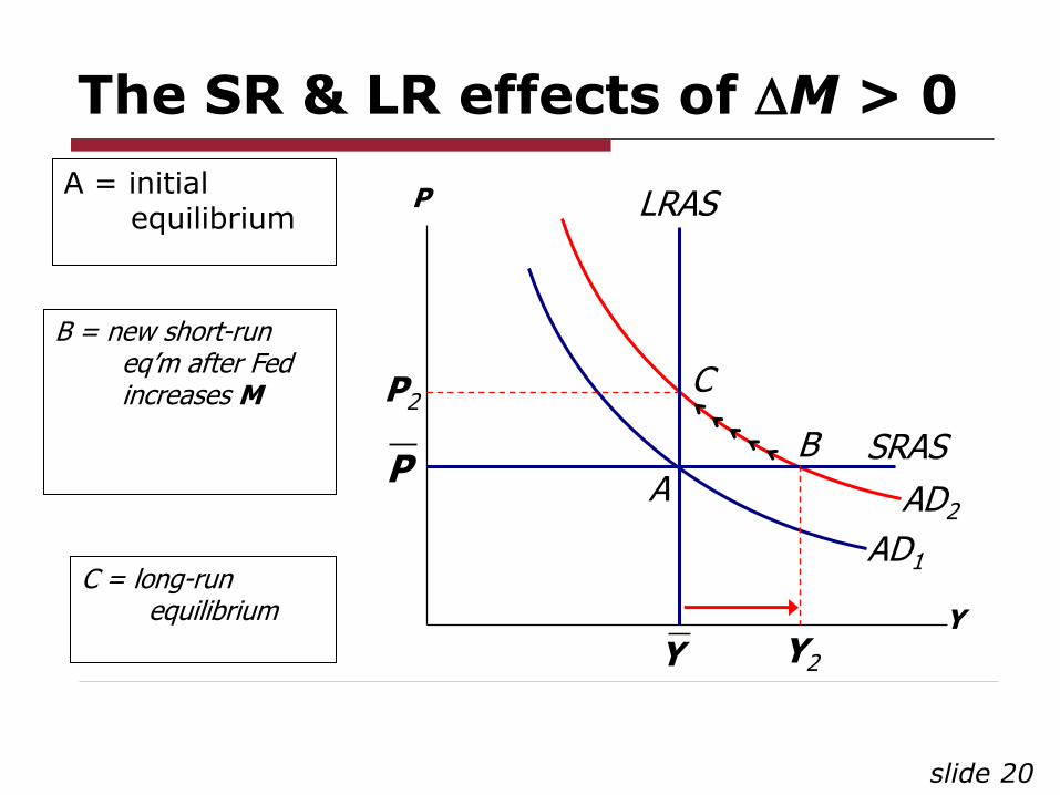
The SR & LR effects of M > 0

Y

P

AD1

AD2

LRAS

Y

PSRAS

P2

Y2

A = initial equilibrium

A

B

C

B = new short-run eq’m after Fed increases M

C = long-run equilibrium

slide 21

How shocking!!!

shocks: exogenous changes in aggregate supply or demand

Shocks temporarily push the economy away from full-employment.

An example of a demand shock: exogenous decrease in velocity

If the money supply is held constant, then a decrease in V means people will be using their money in fewer transactions, causing a decrease in demand for goods and services:

slide 22

LRAS

AD2

PSRAS

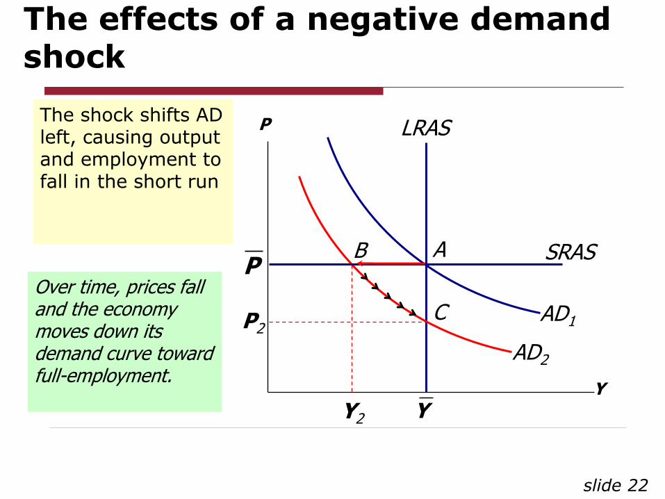
The effects of a negative demand shock

Y

P

AD1

Y

P2

Y2

The shock shifts AD left, causing output and employment to fall in the short run

A B

C

Over time, prices fall and the economy moves down its demand curve toward full-employment.

slide 23

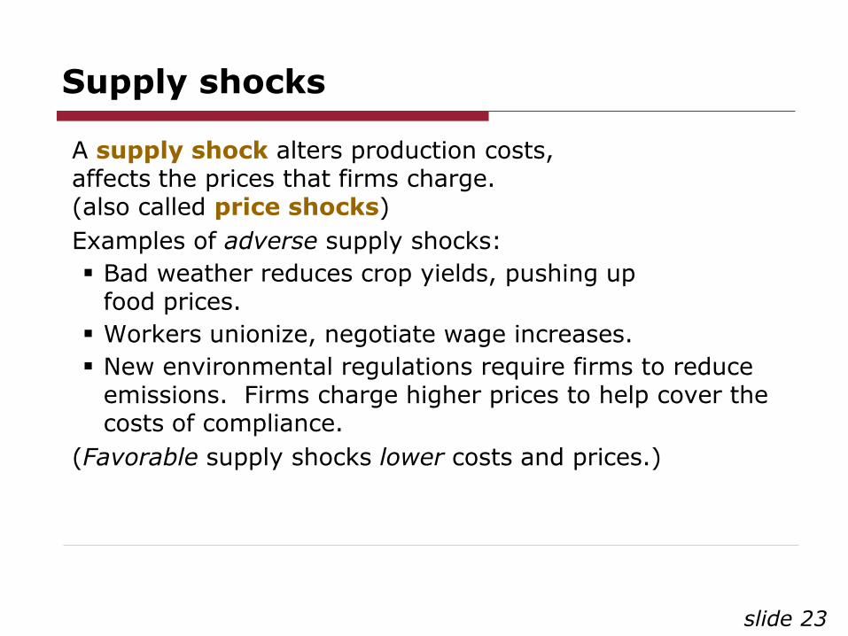
Supply shocks

A supply shock alters production costs, affects the prices that firms charge. (also called price shocks)

Examples of adverse supply shocks:

Bad weather reduces crop yields, pushing up food prices.

Workers unionize, negotiate wage increases.

New environmental regulations require firms to reduce emissions. Firms charge higher prices to help cover the costs of compliance.

(Favorable supply shocks lower costs and prices.)

slide 24

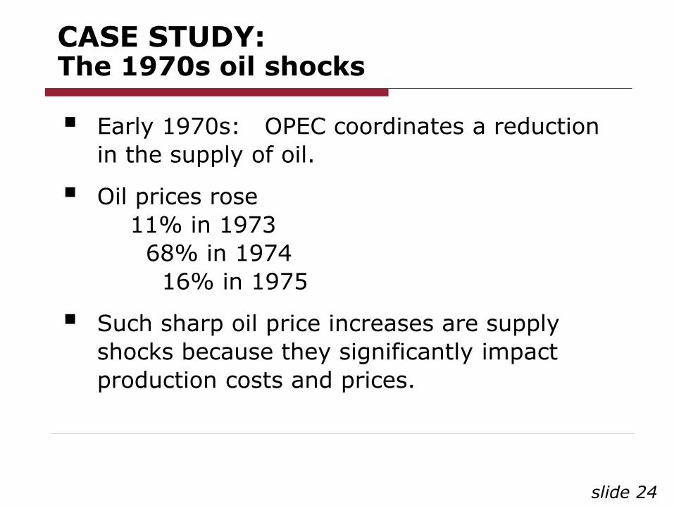
CASE STUDY: The 1970s oil shocks

Early 1970s: OPEC coordinates a reduction

in the supply of oil.

Oil prices rose

11% in 1973

68% in 1974

16% in 1975

Such sharp oil price increases are supply

shocks because they significantly impact

production costs and prices.

slide 25

1PSRAS1

Y

P

AD

LRAS

YY2

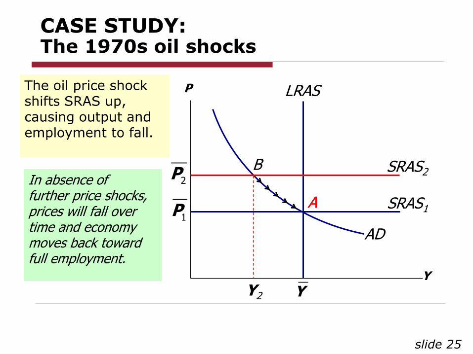
The oil price shock shifts SRAS up, causing output and employment to fall.

A

B In absence of further price shocks, prices will fall over time and economy moves back toward full employment.

2PSRAS2

CASE STUDY: The 1970s oil shocks

A

slide 26

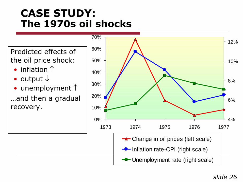
CASE STUDY: The 1970s oil shocks

Predicted effects of

the oil price shock:

• inflation

• output

• unemployment

…and then a gradual

recovery.

0%

10%

20%

30%

40%

50%

60%

70%

1973 1974 1975 1976 1977

4%

6%

8%

10%

12%

Change in oil prices (left scale)

Inflation rate-CPI (right scale)

Unemployment rate (right scale)

slide 27

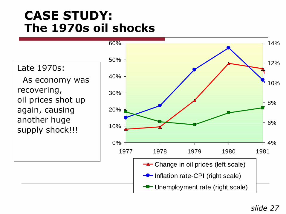
CASE STUDY: The 1970s oil shocks

Late 1970s:

As economy was

recovering,

oil prices shot up

again, causing

another huge

supply shock!!!

0%

10%

20%

30%

40%

50%

60%

1977 1978 1979 1980 1981

4%

6%

8%

10%

12%

14%

Change in oil prices (left scale)

Inflation rate-CPI (right scale)

Unemployment rate (right scale)

slide 28

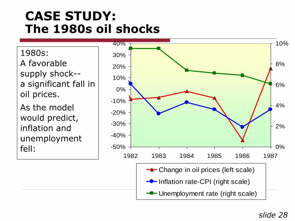
CASE STUDY: The 1980s oil shocks

1980s:

A favorable

supply shock--

a significant fall in

oil prices.

As the model

would predict,

inflation and

unemployment

fell: -50%

-40%

-30%

-20%

-10%

0%

10%

20%

30%

40%

1982 1983 1984 1985 1986 1987

0%

2%

4%

6%

8%

10%

Change in oil prices (left scale)

Inflation rate-CPI (right scale)

Unemployment rate (right scale)

slide 29

Stabilization policy

def: policy actions aimed at reducing the severity of short-run economic fluctuations.

Example: Using monetary policy to combat the effects of adverse supply shocks:

slide 30

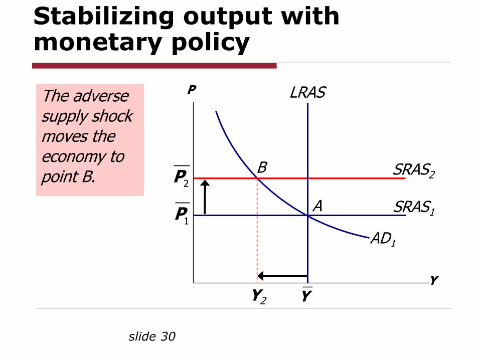
Stabilizing output with monetary policy

1PSRAS1

Y

P

AD1

B 2P

SRAS2

A

Y2

LRAS

Y

The adverse supply shock moves the economy to point B.

slide 31

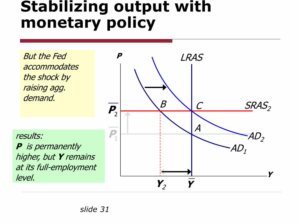
Stabilizing output with monetary policy

1P

Y

P

AD1

B 2P

SRAS2

A

C

Y2

LRAS

Y

AD2

But the Fed accommodates the shock by raising agg. demand.

results: P is permanently higher, but Y remains at its full-employment level.

slide 32

Lecture summary

1. Long run: prices are flexible, output and

employment are always at their natural

rates, and the classical theory applies.

Short run: prices are sticky, shocks can

push output and employment away from

their natural rates.

2. Aggregate demand and supply:

a framework to analyze economic

fluctuations

slide 33

Lecture summary

3. The aggregate demand curve slopes

downward.

4. The long-run aggregate supply curve is

vertical, because output depends on

technology and factor supplies, but not

prices.

5. The short-run aggregate supply curve is

horizontal, because prices are sticky at

predetermined levels.

slide 34

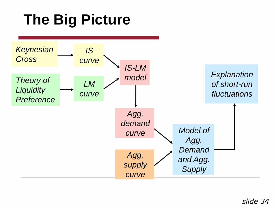
The Big Picture

Keynesian

Cross

Theory of

Liquidity

Preference

IS

curve

LM

curve

IS-LM

model

Agg.

demand

curve

Agg.

supply

curve

Model of

Agg.

Demand

and Agg.

Supply

Explanation

of short-run

fluctuations

Thank you and see you next week!