Lecture 10, Thursday 8.10, Lecture 11, Tuesday 13.10, Lecture 12

Phylogeny inferencePhylogeny inference

Studying evolutionary relatedness among various groups of organisms(species, populations), through molecular sequence data (and also throughmorphological data).

The course Phylogenetic data analysis (period IV, 2010) is an in-depthcourse on this topic

The link: http://evolution.genetics.washington.edu/phylip/software.htmlshows that this field of science is an exceptionally popular one, 385 softwarepackages at the moment.

The most widely used are PHYLIP, PAUP, MEGA, MrBAYES

This lecture starts by a demo with MEGA4 (http://www.megasoftware.net/)and exercise session 5 relates to getting started with (easy) phylogenyreconstructions

8-15. Oct / 1582606 Introduction to Bioinformatics, Autumn 2009

http://evolution.genetics.washington.edu/phylip/software.html

http://www.megasoftware.net/

67

8

Basic concepts and termsBasic concepts and terms________________________________________________________________________________________

Leaves, external nodes 1,2,3,4,5 areobservations which may be, depending on thesituation, sequences from different species,populations etc. They are often called OTUs =Operational Taxonomic Units. Internal nodes6,7,8 are hypothetical sequences in ancestralunits

The tree is unrooted.

In case evidence exists for depicting theroot (for example, a or b), a rooted threecan be constructed.

For example, is there is datafrom different human populationsand from chimpanzee, this animalis an outgroup and a meansfor rooting a tree

Rooting requiresexternal evidence andcannot be done on the basis of the data whichis under a given study.

a b

6

7

8

3

4

5

2

1

a

1 2 3 4 5

b

6

7

8

1 2 3 5 4

582606 Introduction to Bioinformatics, Autumn 2009 8-15. Oct / 2

3

Number of possible rooted and unrooted treesNumber of possible rooted and unrooted trees

n Bn b’n3 1 3

4 3 15

5 15 105

6 105 945

7 954 10395

8 10395 135135

9 135135 2027025

10 2027025 34459425

20 2.22E+020 8.20E+021

30 8.69E+036 4.95E+038

The number of unrooted treesbn = (2(n – 1) – 3)bn-1 = (2n – 5)bn-1 = (2n – 5) * (2n – 7) * …* 3 * 1 = (2n – 5)! / ((n-3)!2n-3), n > 2

Number of rooted trees b’n isb’n = (2n – 3)bn = (2n – 3)! / ((n-2)!2n-2), n > 2

that is, the number of unrooted trees times the number of branches in the trees


Maximum parsimonyMaximum parsimony

EntitiaEntitia nonnon suntsunt multiplicandamultiplicanda praeterpraeter necessitatemnecessitatem

Discrete character states, the shortest pathway leading to these ischosen as the best tree. A model-free method.

Parsimony, Occam´s razor, a philosophical concept, “the best hypothesis isthe one requiring the smallest number of assumptions”.

William of Ockham (1280William of Ockham (1280--1350)1350)


Parsimony analyses have been used from the early 1970s.

The principle of maximum parsimony: identification of a tree topology/topologiesthat require the smallest number of evolutionary changes, i.e. transformations of onecharacter state into another, to explain the differences among OTUs (operationaltaxonomic units).

The goal of minimizing evolutionary change is often defended on philosophicalgrounds: when two hypotheses provide equally valid explanations for a phenomenon,the simpler one should always be preferred.

Two subproblems:(1) determining the amount of character change, or tree length, required by any

given tree(2) searching over all possible tree topologies for the trees that minimize this length.


Informative and uninformative sites______________________________________________

1 2 3 4 5 6 7 8 9OTU a A A G A G T T C AOTU b A G C C G T T C TOTU c A G A T A T C C AOTU d A G A G A T C C T

+ + +

Four OTUs, three possible unrooted trees: I, II, IIItree I ((a,b),(c,d)) tree II ((a,c),(b,d)) tree III ((a,d),(b,c))

site 3 a G A c a G C b a G C bG A A A A A

b C A d c A A d d A A c

site 5 a G A c a G G b a G G bG A A A A A

b G A d c A A d d A A c

site 9 a A A c a A T b a A T bT T A T T T

b T T d c A T d d T A c

A site is informative only when there are at least two different kinds ofnucleotides at the site, each of which is represented in at least two OTUs

A nucleotide site is informativeonly if it favors a subset of treesover the other possible trees.Invariant (1, 6, 8 in the picture)and uninformative sites are notconsidered.

Variable sites:

Site 2 is uninformative becauseall three possible trees require 1evolutionary change, G ->A.

Site 3 is uninformative becauseall trees require 2 changes.

Site 4 is uninformative becauseall trees require 3 changes.

Site 5 is informative becausetree I requires one change, trees IIand III require three changesSite 7 is informative, like site 5

Site 9 is informative because treeII requires one change, trees I andIII require two.


Inferring the maximum parsimony treeInferring the maximum parsimony tree____________________________________________________________________________________________________

Identification of all informative sites and for each possible tree the minimum number ofsubstitutions at each informative site is calculated.

In the example for sites 5, 7 and 9:tree I requires 1, 1, and 2 changestree II requires 2, 2, and 1 changestree III requires 2, 2, and 2 changes.

Summing the number of changes over all the informative sites for each possible tree andchosing the tree associated with the smallest number of changes:

Tree I is chosen because it requires 4 changes, II and III require 5 and 6 changes.

In the case of 4 OTUs an informative site can favor only one of the three possiblealternative trees. For example, site 5 favors tree I over trees II and III, and is thus said tosupport tree I. The tree supported by the largest number of informative sites is the mostparsimonious tree. In the cases where more than 4 OTUs are involved, an informative sitemay favor more than one tree and the maximum parsimony tree may not necessarily be theone supported by the largest number of informative sites.


Exhaustive and heuristic searching for the maximum parsimony treeExhaustive and heuristic searching for the maximum parsimony tree______________________________________________________________________________________________________________________

The total number of substitutions at both informative and uninformative sites in aparticular tree is called the tree length.

When the number of OTUs is small, it is possible to look at all possible trees, determinetheir length, and choose among them the shortest one(s) = exhaustive search.

Large number of sequences (more than about 12) makes exhaustive searchesimpossible.

Short-cut algorithms, for example ´branch-and-bound´: First an arbitrary tree isconsidered (or a tree obtained by another methods, for example some distance method),and compute the minimum number of substitutions for the this tree, which is consideredas the “upper bound” to which the length of any other tree is compared. The rationale isthat the maximum parsimony tree must be either equal in length to this tree or shorter.

Above 20 sequences heuristic searches are needed: only a manageable subset of all thepossible trees is examined. Branch swapping (rearrangement) is used to generatetopologically similar trees from a initial one. Subtree pruning and regrafting is one method.

8-15. Oct / 8

This picture is modified from : Zvelebid&Baum, UnderstandingBioinformatics, 2008, Garland Science, Page 277.

Flow–diagram including thedifferent steps in buildingphylogenetic trees .

Phylogeny reconstructionPhylogeny reconstruction

8-15. Oct / 9

Distance matrix methodsDistance matrix methodsNeighborNeighbor--joining phylogeny by MEGAjoining phylogeny by MEGA--softwaresoftware

Introduction to getting started with phylogenies in practice:exercise session 5 with MEGA-software

8-15. Oct / 10

Introduced in 1960´s, based on clustering algorithms of Sokal and Sneath (1963,Principles of numerical taxonomy).

Calculatation of a measure of the distance between each pair of units (forexample, species) and then finding a tree that predicts the observed set ofdistances as closely as possible.

The data is reduced to a matrix table of pairwise distances, which can beconsidered as estimates of the branch length separating a given pair of unitscompared.

Each distance infers the best unrooted tree for a given pair of units. In effect,there is a number of estimated two-unit trees, and finding the n-unit tree that isimplied is the task.

The individual distances are not exactly the path lengths in the full n-unit treebetween two units: finding the full tree that does the best job of approximatingthe individual two-unit trees.

8-15. Oct / 11

Distances in a phylogenetic treeDistances in a phylogenetic tree__________________________________________________________________________________________________________________

Distance matrix D = (dij) gives pairwise distances for leaves of the phylogenetic tree

In addition, the phylogenetic tree will now specify distances between leaves and internal nodes

Distances dij in evolutionary context satisfy the following conditions:Symmetry: dij = dji for each i, jDistinguishability: dij 0 if and only if i jTriangle inequality: dij dik + dkj for each i, j, kDistances satisfying these conditions are called metricIn addition, evolutionary mechanisms may impose additional constraints on thedistances: additive and ultrametric distances

A tree is called additive, if the distance between any pair of leaves (i, j) is the sum of thedistances between the leaves and a node k on the shortest path from i to j in the tree

dij = dik + djk

A rooted additive tree is called an ultrametric tree, if the distances between any two leaves iand j, and their common ancestor k are equal

dik = djk

Edge length dij corresponds to the time elapsed since divergence of i and j from the commonparent ,i.e. edge lengths are measured by a ”molecular clock” with a constant rate

8-15. Oct / 12

13

Ultrametric treeUltrametric tree

9

8

7

5 4 3 2 1

6

Observation time

Tim

e

Only vertical segments of the tree havecorrespondence to some distance dij:

Horizontal segments act as connectors.d8,9

Distances to be ultrametric can be found by the three-point condition:D corresponds to an ultrametric tree if and only if for any three species(OTUs) i, j and k, the distances satisfy dij max(dik, dkj)

dik = djk for any twoleaves i, j and anyancestor k of i and j

Three-pointcondition: there areno leafs i, j for whichdij > max(dik, djk)for some leaf k.


UPGMA algorithmUPGMA algorithm

Unweighted Pair Group Method using arithmetic Averages, constructs an ultrametricphylogenetic tree via clustering

The algorithm works by at the same time merging two clusters and creating a new node on thetree. The tree is built from leaves towards the root.

NeighborNeighbor--joining algorithmjoining algorithm

Neighbor joining has similarities to UPGMA, Differences in the choice of function f(C1, C2) andhow to assign the distances

Find clusters C1 and C2 that minimise a function f(C1, C2)Join the two clusters C1 and C2 into a new cluster CAdd a node to the tree corresponding to CAssign distances to the new branch

The distance dij for clusters Ci and Cj is

Let u(Ci) be the separation of cluster Ci from other clusters defined bywhere n is the number of clusters.

Instead of trying to choose the clusters Ci and Cj closest to each other, neighbor joiningat the same time

Minimises the distance between clusters Ci and Cj andMaximises the separation of both Ci and Cj from other clusters


This picture is from : Zvelebid&Baum, Understanding Bioinformatics, 2008,Garland Science, Page 279.

UPGMA-method,a worked example

Tree reconstruction from six sequences, A-F.(A) The distance matrix showing that A and D are closest. Theyare selected in the first step to produce internal node V (in (B)).(B) The distance matrix including node V from which it can bededuced that V and E are closest, resulting in internal node W.(C,D) Subsequent steps defining nodes X, Y and Z and resultingin the final tree (E).


This picture is from : 277. Zvelebid&Baum, Understanding Bioinformatics,2008, Garland Science, Page 281.

Fitch-Margoliash method, NOTE: Thisdistance-method not in MEGA-software

(A) In the first step the shortest distance is used to identifythe two clusters (A,C) which are combined to create the nextinternal node. A temporary cluster (W) is defined as allclusters except these two, and the distances calculated fromW to both A and C. The method then uses equations b1 = ½(d

AB + d AC – d BC, b 2 = ½(d AB + d BC – d AC), b 3 = ½(d AC + d BC – D

AB) to calculate the branch lengths from A and C to theinternal node that connects them. (B) A and C are combinedinto the cluster X and the distances calculated from the otherclusters. After identifying B and X as the next clusters to becombined to create cluster Z, the temporary cluster Y containsall other sequences. X is the distance b3 from the new internalnode, and the distance between the internal nodes is b4.Branch length b4 is negative (not realistic); in futurecalculations this branch is treated like

all others. (C) Combining sequences A,B and Cinto cluster Z, the sequences D and E areadded to the tree in the final step. (D) The finaltree has a negative branch length. The tablesgive the patristic distances (those measurer onthe tree itself) and the errors (eij). The tree hasa wrong topology,

as becomes clear with the neighbor-joining tree from the same data.


This picture is from : Zvelebid&Baum, Understanding Bioinformatics, 2008,Garland Science, Page 284.

Neighbor-joining method,a worked example

The distance matrix is the same as in the Fitch-Margoliashexample.At each step the distances are converted by using the algorithmwhich minimizes the total tree distance (the minimum evolutionprinciple).

The first step:

(A) Star-tree in which all sequences are joined directly to asingle internal node X with no internal branches.

(B) After sequences 1 and 2 have been identified as the firstpair of nearest-neighbors, they are separated from node Xby and internal node Y. The method calculates the brabchlengths from sequences 1 and 2 to node Y to complete thestep.


Parameters of nucleotide changeParameters of nucleotide change

____________________________________________________________________________________________________________________________________

One-parameter model, the ´Jukes-Cantor model´

Assumption: nucleotide substitutions occur with equal probabilites,

The rate of substitution for each nucleotide is 3 per unit time

A T C G

A

T

C

G

At time 0: A at a certain nucleotide site, PA(0) = 1Question: probability that this site is occupied by A at time t , PA(t) ?At time 1, probability of still having A at this site is

PA(1) = 1 - 3 (1)

is the probability of A changing to T, C, or G


The probability of the site having A at time 2 is

PA(2) = (1 - 3 )P(A1) + [1 – PA(1)] (2)

This includes two possible course of events:

t = 0 t = 1 t = 2A A A

no substitution no substitution

A T, C or G Asubstitution substitution

The following recurrence equation applies to any t

PA(t+1) = (1 - 3 )PA(t) + [1 – PA(t) ] (3)

Note that this holds also for t = 0, because PA(0) = 1 and thusPA(0+1) = (1 – 3 ) PA(0) + [1 – PA(0) ] = 1 - 3which is identical with equation (1).


The amount of change per unit time, rewriting equation (3):

PA(t) = PA(t+1) – PA(t) = - 3 PA(t) + [1 – PA(t) ] = - 4 PA(t) + (4)

Approximating the previous discrete-time model by a continuous-time model, byregarding PA(t) as the rate of change at time t

dPA(t) / dt = - 4 PA(t) + (5)

The solution of this first-order linear differential equation is

PA(t) = ¼ + (PA(0) – ¼ )e -4 t (6)

The starting condition was A at the given site, P A(0) = 1, consequently

PA(t) = ¼ + ¾ e -4 t (7)

Equation holds regardless of the initial conditions, for example if the initialnucleotide is not A, then PA(0) = 0, and the probability of having A at time t

PA(t) = ¼ + ¼ e -4 t (8)


Equations (7) and (8) describe the substitution process. If the initial nucleotide isA, then PA(t) decreases exponentially from 1 to ¼ . If the initial nucleotide is not A,then PA(t) will increase monotonically from 0 to ¼ .

Under this simple model, after reaching equilibrium, PA(t)=PT(t)=PC(t)=PG(t) for allsubsequent times.

Equation (7) can be rewritten in a more explicit form to take into account that theinitial nucleotide is A and the nucleotide at time t is also A

PAA(t) = ¼ + ¾ e -4 t (9)

If the initial nucleotide is G instead of A, from equation (8)

PGA(t) = ¼ + ¼ e -4 t (10)

Since all the nucleotides are equivalent under the Jukes-Cantor model, the generalprobability, Pij(t) , that a nucleotide will become j at time t, given that it was i at time 0,equations (9) and (10) give the general probabilities Pii(t) andPij(t), where i j.


KimuraKimura´́s twos two-- parameterparameter --modelmodel

The Jukes-Cantor –model was introduced in 1969 when virtually nothing was knownabout nucleotide substitution

In 1980 Kimura proposed different parameters for transitions and transversions.

Transition is a nucleotide change between purines, A and G, and pyrimidines, T and C.Transversion is a purine – pyrimide change.

The rate of transition change is and transversion change is per unit time

A T C G

A

T

C

G


The development of models of sequence evolution is a very active field, profuseamount of publications.

Two approaches:

Empirically using properties calculated through comparisons of largenumbers of observed sequences. For example simply countingapparent replacements between many closely related sequences.

Empirical models result in fixed parameter values which areestimated only once and the n assumed to be applicable to alldatasets => computationally easy to use

Parametrically on the basis of the chemical or biologicalproperties of DNA and amino acids. For example, incorporating aparameter to describe the relative frequency of transition (purine- purine,pyrimidine-pyrimidine) and transversion (purine –pyrimidine).

Parameter values are derived from the dataset in each particularanalysis.

Both methods result in Markov process models, defined by matrices containing therelative rates (=the relative numbers, on average, and per unit time). From these arecalculated the probabilities of change from any nucleotide to any other nucleotide,including the probability of remaining the same, over any period of evolutionary timeat any site


Relationships among six standard modelsof nucleotide evolution.

For each model the matrix of rates of substitutionsbetween nucleotides is shown (represented by abubble plot where the area of each bubble indicatesthe corresponding rate), a partial representation of ahominoid phylogeny as inferred by that model froma mitochondrial sequence dataset, and themaximum log-likelihood value obtained. For theREV+ model also the gamma distribution of ratesamong sites described by the inferred parametervalue =0.28 is shown. The reverse-J shape of thegraph indicates that the majority of sites have lowrates of evolution, with some sites having high ratesof evolution. The JC model assumes that allnucleotide substitutions occur at equal rates. Themodels become more advanced moving down thefigure, as illustrated in the bubble plots by theirincreasing flexibility in estimating relativereplacement rates and as reflected by increasing log-likelihoods. Note how the inferred maximumlikelihood phylogeny changes significantly as themodels become more advanced (compare JC withK2P); inferred branch lengths also tend to increase(compare REV to REV+ ). Arrows show wheremodels are nested within each other; that is, wherethe first model is a simpler form of the next. Forexample, the JC model is nested within the K2Pmodel (it is a special case arising when is fixedequal to 1), but the K2P model is not nested with theFEL model.


Model comparisons

The likelihood framework permits estimation of parameter values and their standarderrors from the observed data (with no need for any a priori knowledge).

For example, a transition / transversion bias estimated as = 2.3 +/- 0.16 effectivelyexcludes the possibility that there is no such bias ( = 1), whereas = 2.3 +/- 1.6 doesnot.

Likelihood ratio tests compare two competing models, using their maximizedlikelihoods with a statistic, 2 , that measures how much better an explanation of thedata the alternative model gives. To perform a significance test, the distribution ofvalues of 2 expected under the simpler hypothesis is required. If the observed valueof is too great to be consistent with this distribution (P-values), the simpler modelis rejected in favour of the more complex model.

When two models being compared are nested, the simpler model being a specialcase of the more complex model obtained by constraining certain free parameters totake particular values, then the required distribution for 2 is usually a 2 distributionwith the number of degrees of freedom equal to the difference in the number ofparameters between the two models.


When the models are not nested (the usual situation with complex models)the required distribution of 2 can be estimated by Monte Carlo simulation orparametric bootstrapping.

Figure in the next page illustrates a test for assessing whether one particularmodel is a statistically adequate description of the evolution of a set ofsequences.

This test almost invariably indicates that current models of sequenceevolution are not explaining the evolutionary patterns in the data fully(sequences have been evolving by natural selection


Statistical tests of models.

(a) Part of the mitochondrial sequence datasetused in previous figure, and the maximumlikelihood phylogenetic tree and likelihoodvalues from the HKY) and REV models.

(b) The statistical test to compare these modelsof nucleotide substitution, in which thelikelihood ratio statistic 2 is compared with a42 distribution. The observed value of 2 , 14.4,

has a P-value considerably less than 0.05, andthe HKY model is rejected in favour of the REVmodel.

(c) The test of the adequacy of the REV model.The test statistic is derived from a comparisonof the REV model and a multinomial model thatidentifies the maximum possible likelihoodattainable under any model. The testdistribution is estimated by parametricbootstrapping, in which simulated datasets Si

(generated using the maximum likelihoodphylogeny and substitution model parametersestimated with the REV model) and aresubjected to the same analysis as the originaldata. Comparison of the test statistic and thedistribution of values obtained from simulateddata indicates that the observed value 2 is farin excess of what is expected if the REV modelwere accurate, and we can conclude that amore complex evolutionary model is necessaryto describe the patterns of evolution of these

sequences fully.


Considering the primary interest in the topology of the inferredevolutionary tree:

As with estimates of model parameters, a single point-estimate is of little value without some measure of theconfidence.

Non-parametric bootstrapping: comparisons of an inferredtree with a set of bootstrap replicate trees, typically in theform of tabulation of the proportion of the bootstrap replicatesin which each branch from the inferred tree occurs.

Difficulty in the precise interpretation of what these valuesrepresent.


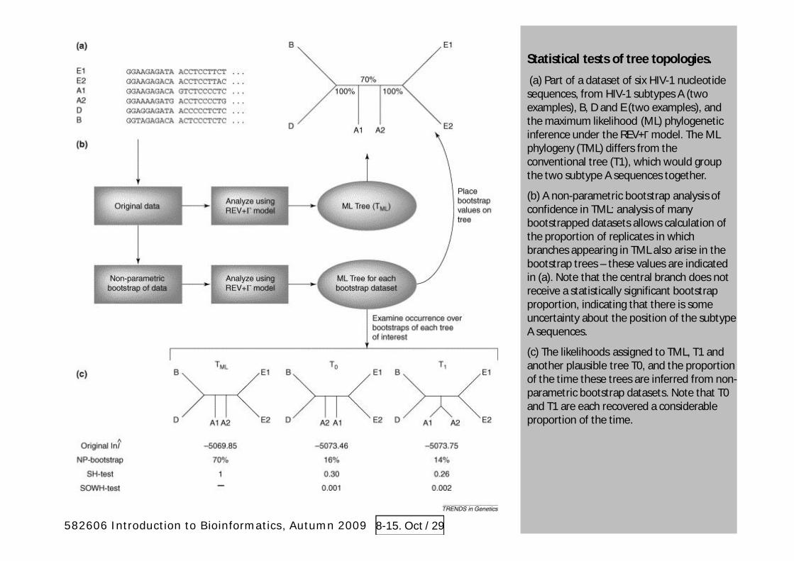
Statistical tests of tree topologies.

(a) Part of a dataset of six HIV-1 nucleotidesequences, from HIV-1 subtypes A (twoexamples), B, D and E (two examples), andthe maximum likelihood (ML) phylogeneticinference under the REV+ model. The MLphylogeny (TML) differs from theconventional tree (T1), which would groupthe two subtype A sequences together.

(b) A non-parametric bootstrap analysis ofconfidence in TML: analysis of manybootstrapped datasets allows calculation ofthe proportion of replicates in whichbranches appearing in TML also arise in thebootstrap trees – these values are indicatedin (a). Note that the central branch does notreceive a statistically significant bootstrapproportion, indicating that there is someuncertainty about the position of the subtypeA sequences.

(c) The likelihoods assigned to TML, T1 andanother plausible tree T0, and the proportionof the time these trees are inferred from non-parametric bootstrap datasets. Note that T0and T1 are each recovered a considerableproportion of the time.



FrequentistFrequentist and Bayesian tree confidence and credibilityand Bayesian tree confidence and credibility

Quantifying the uncertainty of a phylogenetic estimate is at least as important a goal as obtaining thephylogenetic estimate itself.

Measures of phylogenetic reliability point out what parts of a tree can be trusted when interpreting theevolution of a group and guide future efforts in data collection that can help resolve remaining uncertainties.

Bootstrapping (in distance methods and in maximum likelihood phylogenies) and posterior probability (inBayesian phylogenies)


Bootstrapping proceduce

Sample 1 2 3 4 5 6 7 8 9 10 11 12 13 14 15 16 17 18 19 20

OTU 1 G A G G G A G G A C C C G A T C A A A A

OTU 2 G C G T G G G G A A C C G G A G A A A C

OTU 3 C A A A G A G C A A C G A G T T A A A C

OTU 4 G C G G A C A G A A A A G A T T A A A T

OUT 5 C A G A G A G A A A C A G A G T A A A C

Pseudosample 1 1 1 1 1 2 6 6 6 8 8 10 13 13 13 13 15 16 17 17 19

3 1

2

4 5

Pseudosample 2 2 2 2 2 5 7 8 8 9 10 11 12 12 14 14 17 17 18 20 20

3 1

2

4 5

Pseudosample 3 3 3 3 5 5 6 7 7 9 9 11 11 11 11 11 12 12 18 18 18

5 3

2

4

1


Strict Consensus Tree

Hu Ch Go Or Gi Hu Ch Go Or Gi

Tree 1 Tree 3

Hu Ch Go Or Gi

Tree 2

Hu Ch Go Or Gi


Majority Rule Consensus Tree

Hu Ch Go Or Gi Hu Ch Go Or Gi

Tree 1 Tree 3

Hu Ch Go Or Gi

Tree 2

Hu Ch Go Or Gi


The bootstrapping approach .When optimality-criterionmethods are used, a tree search (green box) is performedfor each data set, and the resulting tree is added to the finalcollection of trees. A wide variety of tree-search strategieshave been developed, but most are variants of the samebasic strategy. An initial tree is chosen, either randomly oras the result of an algorithm — such as neighbour joining .Changes to this tree are proposed; the type of move can beselected randomly or the search can involve trying everypossible variant of a particular type of move .The new tree isscored and possibly accepted. Some search strategies arestrict hill-climbers — they never accept moves that result inlower scores; others (genetic algorithms or simulatedannealing) occasionally accept worse trees in an attempt toexplore the tree space more fully.

The Markov chain Monte Carlo (MCMC) methodology is similarto the tree-searching algorithm, but the rules are stricter. From aninitial tree, a new tree is proposed. The moves that change thetree must involve a random choice that satisfies severalconditions. The MCMC algorithm also specifies the rules for whento accept or reject a tree. MCMC yields a much larger sample oftrees in the same computational time, because it produces onetree for every proposal cycle versus one tree per tree search(which assesses numerous alternative trees) in the traditionalapproach. However, the sample of trees produced by MCMC ishighly auto-correlated. As a result, millions of cycles throughMCMC are usually required, whereas many fewer (of the order of1,000) bootstrap replicates are sufficient for most problems.


1) A classical example: phylogenetics in court

Molecular evidence of HIV-1 transmission in a criminal caseBy: Metzker et al., PNAS October 29, 2002, 99: 14292-14297. doi: 10.1073/pnas.222522599

A gastroenterologist was convicted of attempted second-degree murder by injecting his former girlfriend withblood or blood-products obtained from an HIV type 1 (HIV-1)-infected patient under his care.

Phylogenetic analyses of HIV-1 sequences were admitted and used as evidence in this case, representing thefirst use of phylogenetic analyses in a criminal court case in the United States.

Phylogenetic analyses of HIV-1 reverse transcriptase and env DNA sequences isolated from the victim, thepatient, and a local population sample of HIV-1-positive individuals showed the victim's HIV-1 sequences to bemost closely related to and nested within a lineage comprised of the patient's HIV-1 sequences.

Examples of phylogeny inference in practiceExamples of phylogeny inference in practiceExamples of phylogeny inference in practiceExamples of phylogeny inference in practice


Phylogenetic analyses of the gp120 and RT sequences (two genes of the virus) to examinerelationships among the patient, victim, and LA (geographical reference area) control viral DNAsequences. The analyses that formed the basis of the results we presented in court were conductedby using the optimality criteria of parsimony and minimum evolution (neighbor joining algorithm).

These approaches were used because they were accepted by the court in a pre-trial hearing asmeeting the criteria for admissibility of evidence. Analyses based on direct likelihood evaluations ofthe sequence data were not computationally feasible at the time of the pretrial hearing or court case.

Recent developments of Markov-chain Monte Carlo (MCMC) approaches have, however, made aBayesian analysis under a likelihood model feasible. Therefore, additional post-trial analyses wereconducted with MCMC Bayesian analysis by using the Metropolis-coupled MCMC algorithmimplemented in the program mrBayes.

Bayesian analysis was based on a General-Time-Reversible model of sequence evolution, with -distributed rate heterogeneity among sites and a calculated proportion of invariable sites (GTR+ +I).

For each gene, 5,000,000 MCMC generations, and sampled solutions once every 100 generations.After 2,500,000 generations, it was determined that the searches had reached equilibrium by plottingthe values for the likelihood scores and the various parameters of the model. We therefore used thesamples from the final 2,500,000 generations to compute 95% confidence intervals for the modelparameters shown in Tables (next page), and to assess the posterior probabilities of the relationshipsbetween the victim and patient sequences.

Note that the two genes are very different (see the parameter estimates). This serves here as anexample of the importance of models (cf. above, the simple Jukes-Cantor model would not beadequate).


Means and 95% confidence intervals for parameters of the GTR + + I model forgp120 sequences (one gene from the virus)

Parameter Mean 95% confidence interval-------------------------------------------------------------------------------------------------------------C–T substitution rate 5.03 3.60–7.03C–G substitution rate 0.97 0.57–1.54A–T substitution rate .75 0.52–1.07A–G substitution rate 3.87 91–5.10A–C substitution rate 2.34 1.60–3.34Frequency of A 0.40 0.37–0.43Frequency of C 0.15 0.13–0.17Frequency of G 0.23 0.21–0.25Frequency of T 0.22 0.20–0.25

(shape of distribution) 0.53 0.43–0.68Proportion of invariable sites 0.08 0.01–0.18

Means and 95% confidence intervals for parameters of the GTR + + I model for the RT sequences(another gene from the virus)

Parameter Mean 95% Confidence interval__________________________________________________________________________C–T substitution rate 110.36 23.04–195.53C–G substitution rate 17.59 2.82–42.02A–T substitution rate 7.62 1.34–17.32A–G substitution rate 83.01 16.29–171.17A–C substitution rate 16.60 3.41–35.62Frequency of A 0.40 0.36–0.43Frequency of C 0.17 0.14–0.19Frequency of G 0.20 0.17–0.23Frequency of T 0.23 0.20–0.26

(shape of distribution) 0.94 0.38–1.94Proportion of invariable sites 0.50 0.29–0.63


For the parsimony and minimum evolution analyses, nonparametric bootstrapping was used to test the a priorihypothesis of a relationship between the victim and patient sequences. The generally accepted standard forrejecting a null hypothesis (in this case, the null hypothesis is that the sequences obtained from the victim are notmost closely related to sequences obtained from the patient) is P < 0.05.

In forensic studies, however, there is no widely accepted standard for the meaning of beyond a reasonabledoubt. Under a wide range of conditions, bootstrap proportions (BP) have been shown to represent a conservativeestimate of phylogenetic confidence, and 1-BP was used as a conservative estimate of p (the probability of type Ierror) in a test of the a priori hypothesis . Because of the importance of estimating the strength of the results, asmany bootstrap replications as were computationally feasible for each analysis were constructed.

For parsimony analyses, 100,000 bootstrap replicates, whereas for the more computationally intense maximum-likelihood distance analyses (in which large numbers of pairwise distances had to be recalculated for eachreplicate), 1,000 (gp120) to 10,000 (RT) replicates.

In the parsimony analyses, all 100,000 bootstrap replicates of the gp120 gene data supported the victim andpatient sequences as the most closely related within the analysis (P < 0.00001), and 95,826 bootstrap replicates ofthe RT gene data supported the victim sequences as embedded within a group of patient sequences (P <0.04174).

In the maximum-likelihood distance analyses, all 1,000 bootstrap replicates of the gp120 gene data (P < 0.001)supported the closer relationship between the patient and victim viral sequences compared with any of the LAcontrols, and all 10,000 bootstrap replicates of the RT gene data (P < 0.0001) supported the victim sequences asembedded within a group of patient sequences. All 25,000 sampled trees from the MCMC analyses also supportedthese relationships (P < 0.00004). The relationships of the patient and victim RT sequences were virtually identicalbased on both the originally sampled sequences (sequenced at BCM) and those subsequently sequenced at another laboratory. (NOTE: Maximum likelihood and Bayesian phylogenies have not been introduced during thisIntroduction to bioinformatics course.)

The close relationship between the victim and patient samples was thus supported by both of the genesthat we examined, using all major methods of phylogenetic analysis (parsimony, minimum evolution, andlikelihood), and a broad range of evolutionary models.


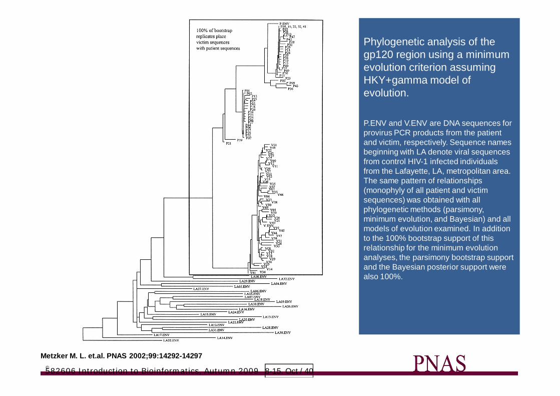
Metzker M. L. et.al. PNAS 2002;99:14292-14297©

Phylogenetic analysis of thegp120 region using a minimumevolution criterion assumingHKY+gamma model ofevolution.

P.ENV and V.ENV are DNA sequences forprovirus PCR products from the patientand victim, respectively. Sequence namesbeginning with LA denote viral sequencesfrom control HIV-1 infected individualsfrom the Lafayette, LA, metropolitan area.The same pattern of relationships(monophyly of all patient and victimsequences) was obtained with allphylogenetic methods (parsimony,minimum evolution, and Bayesian) and allmodels of evolution examined. In additionto the 100% bootstrap support of thisrelationship for the minimum evolutionanalyses, the parsimony bootstrap supportand the Bayesian posterior support werealso 100%.


Metzker M. L. et.al. PNAS 2002;99:14292-14297

Phylogenetic analysis of the RTregion; details of the analysis are thesame as for previous page.

(a) Tree based on sequences fromBCM .

(b) Subtree of patient and victimsequences, including thoseadded by MIC. In both a and b,the smaller set of boxedsequences represents thesequences from the victim, andthe larger set of boxedsequences represents thepatient plus victim sequences.The victim sequences werefound to be embedded withinthe patient sequences in allanalyses and for all models ofevolution examined. In additionto the 100% bootstrap supportof this relationship for theminimum evolution analyses,the parsimony bootstrap supportwas 96% and the Bayesianposterior support was 100%.


(A) Prevaccination measles dynamics:weekly case reports for Leeds, UK.

(B) Weekly reports of influenza-likeillness for France.

(C) Annual diagnosed cases of HIV inthe United Kingdom.

(D) Measles phylogeny: the measlesvirus nucleocapsid gene [63sequences, 1575 base pairs (bp)].

(E) Influenza phylogeny: the humaninfluenza A virus (subtype H3N2)hemagglutinin (HA1) genelongitudinally sampled over aperiod of 32 years (50 sequences,1080 bp).

(F) Dengue phylogeny: the denguevirus envelope gene from all fourserotypes (DENV-1 to DENV-4, 120sequences, 1485 bp).

(G) HIV-1 population phylogeny: thesubtype B envelope (E) genesampled from different patients(39 sequences, 2979 bp).

(H) HCV population phylogeny: thevirus genotype 1b E1E2 genesampled from different patients(65 sequences, 1677 bp).

(I) HIV-1 within-host phylogeny: thepartial envelope (E) genelongitudinally sampled from asingle patient over 5.8 years.

2) Phylodynamics: understanding the behaviour of2) Phylodynamics: understanding the behaviour ofviruses, what happens to their gene sequences duringviruses, what happens to their gene sequences duringtime epochstime epochs



3)3) Resolving the ”tree of life”, the dream of DarwinResolving the ”tree of life”, the dream of Darwin

Genome analyses are delivering unprecedented amounts of data from an abundance of organisms, raisingexpectations that in the near future, resolving the tree of life (TOL) will simply be a matter of data collection. However,recent analyses of some key clades in life's history have produced “bushes” and not resolved trees. The patterns observedin these clades are both important signals of biological history and symptoms of fundamental challenges that must beconfronted.

The combination of the spacing of cladogenetic events and the high frequency of independently evolved characters(homoplasy) limit the resolution of ancient divergences. Because some histories may not be resolvable by even vastincreases in amounts of conventional data, the identification of new molecular characters will be crucial to futureprogress.

The famous science writer, Richard Dawkins says: … “there is, after all, one true tree of life, the unique pattern ofevolutionary branchings that actually happened. It exists. It is in principle knowable. We don't know it all yet. By 2050 weshould – or if we do not, we shall have been defeated only at the terminal twigs, by the sheer number of species.”

Examples of open questions: Who are tetrapods' (four-legged animals) closest living relatives? Which is the earliest-branching animal phylum? Answers to such fundamental questions would be easy if the historical connections among allliving organisms in the TOL were known. Obtaining an accurate depiction of the evolutionary history of all living organismshas been and remains one of biology's great challenges. The discipline primarily responsible for assembling the TOL—molecular systematics—has produced many new insights by illuminating episodes in life's history, posing new hypotheses,as well as providing the evolutionary framework within which new discoveries can be interpreted.

The TOL has been molded by cladogenesis and extinction. Starting from a single lineage that undergoes cladogenesisand splits into two, the rate at which the lineages arising from this cladogenetic event undergo further cladogeneticevents determines the lengths of the nascent stems. Once these stems have been generated, the only process that canmodify their lengths is extinction. At its core, the elucidation of evolutionary relationships is the identification, throughstatistical means, of the tree's stems

(A) Early in a clade's history (gray box), the number of cladogenetic events is smaller and the length of stems larger in tree-like (left) relativeto bush-like clades (right).(B) In the absence of homoplasy, the number of PICs (parsimony informatice characters) for a stem is proportional to its time span; manyPICs (rectangles) accumulated on the long stem x (left), whereas few PICs accumulated on the short stem y (right).(C) When the stem time span is long, the effect of homoplastic characters (crosses supporting a clade of species A and C and bulletssupporting a clade of species B and C) is not sufficient to obscure the true signal (left). In contrast, the same number of homoplasticcharacters is sufficient to mislead reconstruction of short stems (right), because the number of homoplastic characters shared betweenspecies A and C (three crosses in each of the two species) is larger than the number of true PICs (two rectangles).

Homoplasy, homoplastic = the probability of several species acquiring the same nucleotide or amino acid independently.

From: Bushes in the Tree of Life, Rokas A, Carroll SB PLoS Biology Vol. 4, No. 11, e352 doi:10.1371/journal.pbio.0040352


(A) The human/chimpanzee/gorillatree (5–8 million years ago).(B) The elephant/sirenian/hyraxbush (57–65 million years ago).(C) Thetetrapod/coelacanth/lungfish bush(370–390 million years ago).(D) The metazoan superbush (>550million years ago).

In each panel, the three alternativetopologies for each set of taxa areshown. Below each topology, thepercentage and number (inparentheses) of genes, PICs, andRGCs (rare genomic changes)supporting that topology are shown(when available). Numbers ofgenes supporting each topology in(A), (C), and (D) are based onmaximum likelihood analyses;numbers in (B) are based onparsimony. The observed conflictsare not dependent on theoptimality criterion used; similarresults have been obtained byanalyses of the data under a varietyof widely used optimality criteria.A fraction of genes in each panel isuninformative: (A), 6 of 98 genes;(B), 9 of 20 nuclear genes; (C), 1 of44 genes; and (D), 179 of 507genes.

From: Bushes in the tree of life,Rokas A, Carroll SB PLoS BiologyVol. 4, No. 11, e352doi:10.1371/journal.pbio.0040352

4)4) The phylomeThe phylome

Complementing the concepts- transcriptome- proteome- interactome- metabolome

Reconstruction of the evolutionary histories of all genes encoded in agenome

The human phylome- Genome Biology 8:R109 (2007)- proteins encoded by 39 publicly available eukaryotic genomes

Schematic representation of thephylogenetic pipeline used toreconstruct the human phylome. Eachprotein sequence encoded in thehuman genome is compared against adatabase of proteins from 39 fullysequenced eukaryotic genomes toselect putative homologous proteins.Groups of homologous sequences arealigned and subsequently trimmed toremove gap-rich regions. The refinedalignment is used to build a NJ tree,which is then used as a seed tree toperform a ML likelihood analysis asimplemented in PhyML, using fourdifferent evolutionary models (five inthe case of mitochondrially encodedproteins). The ML tree with themaximum likelihood is further refinedwith a Bayesian analysis using MrBayes.Finally, different algorithms are used tosearch for specific topologies in thephylome or to define orthology andparalogy relationships.

From:Huerta-Cepas et al. Genome Biology 20078:R109 doi:10.1186/gb-2007-8-6-r109


5)5) Phylogenetic inference may form a framework for understandingPhylogenetic inference may form a framework for understandingthe evolution of characters, e.g. humanenness....the evolution of characters, e.g. humanenness....

During the course of evolution, gene families have increase their size through events of geneduplication.

These events may correspond to massive duplications affecting many genes in the genome at the sametime, such as in whole genome duplications (WGDs) or may be restricted to chromosomal segments orspecific genes.

Not only recent genomics surveys have provided evidence for the abundance of duplicated genes in allorganisms, but it has also been observed that gene duplication is often associated with processes of neo-functionalization and/or sub-functionalization.

To quantify the extent of gene duplication that has occurred in the lineages leading to human, thephylogenetic trees have been scanned to find duplication events, which have been mapped onto aspecies phylogeny that marks the major branching points in the lineage leading to hominids (next page).

High duplication rates in the lineages leading to mammals, primates and hominids. This suggests thatduplications have played a major role in the evolution of these groups.

Estimates for the number ofduplication events occurredat each major transition inthe evolution of theeukaryotes.Horizontal bars indicate theaverage number ofduplications per gene. Boxeson the right list some of theGO terms of the biologicalprocess category that aresignificantly over-representedcompared to the rest of thegenome in the set of genefamilies duplicated at acertain stage.

GO = gene ontology

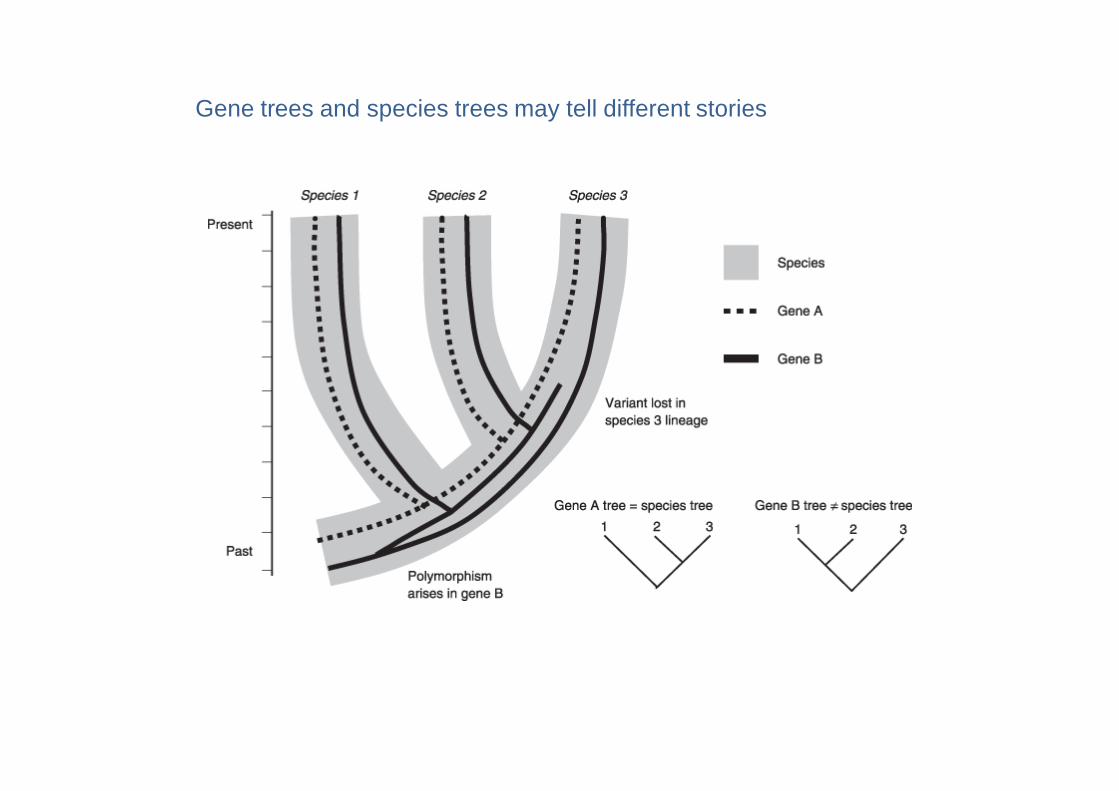
Gene trees and species trees may tell different stories

What is known about humanWhat is known about human--specific charactersspecific characters

“Protein evolution” –related characters usuallymean that acceleratedevolution, “positiveselection”, has beennoticed.

This means that thephylogeny on the basis ofsuch a gene is biased,i.e. has too long branchesas compared to thephylogeny which isknown to reflect evolutionof e.g. “neutral”characters (markerswhich measure elapsedtime).


Human chromosomes, somegenes shown.

Genes with blue colour arethose in which positive selectionhas been inferred.

This field of science is veryactive and is one example of theutilization of phylogeny inference asa tool – the scientific question isnot:

”what is the phylogeny”

but is:” the species phylogeny

should be .... however, it is not (toolong branches, for example), why?Maybe this gene has experiencedhigh rate of evolution and is thusone marker for something specificthat has occurred in the history ofhuman lineage?

Documents

Lecture 10, Thursday 8.10, Lecture 11, Tuesday 13.10, Lecture 12