Embed Size (px)
Citation preview

Statistics 514: 2k Factorial Design
Lecture 10: 2k Factorial Design
Montgomery: Chapter 6
Fall , 2005Page 1

Statistics 514: 2k Factorial Design
2k Factorial Design
• Involving k factors
• Each factor has two levels (often labeled + and −)
• Factor screening experiment (preliminary study)
• Identify important factors and their interactions
• Interaction (of any order) has ONE degree of freedom
• Factors need not be on numeric scale
• Ordinary regression model can be employed
y = β0 + β1x1 + β2x2 + β12x1x2 + ε
Where β1, β2 and β12 are related to main effects, interaction effects defined
later.
Fall , 2005Page 2

Statistics 514: 2k Factorial Design
22 Factorial Design
Example:
factor replicate
A B treatment 1 2 3 mean
− − (1) 28 25 27 80/3
+ − a 36 32 32 100/3
− + b 18 19 23 60/3
+ + ab 31 30 29 90/3
• Let y(A+), y(A−), y(B+) and y(B−) be the level means of A and B.
• Let y(A−B−), y(A+B−), y(A−B+) and y(A+B+) be the treatment
means
Fall , 2005Page 3

Statistics 514: 2k Factorial Design
Define main effects of A (denoted again by A ) as follows:
A = m.e.(A) = y(A+) − y(A−)
= 12 (y(A+B+) + y(A+B−)) − 1
2 (y(A−B+) + y(A−B−))= 1
2 (y(A+B+) + y(A+B−) − y(A−B+) − y(A−B−))= 1
2 (−y(A−B−) + y(A+B−) − y(A−B+) + y(A+B+))=8.33
• Let CA=(-1,1,-1,1), a contrast on treatment mean responses, then
m.e.(A)= 12 CA
• Notice that
A = m.e.(A) = (y(A+) − y..) − (y(A−) − y..) = τ2 − τ1
Main effect is defined in a different way than Chapter 5. But they are
connected and equivalent.
Fall , 2005Page 4

Statistics 514: 2k Factorial Design
• Similarly
B = m.e.(B) = y(B+) − y(B−)
= 12(−y(A−B−) − y(A+B−)) + y(A−B+) + y(A+B+) =-5.00
Let CB=(-1,-1,1,1), a contrast on treatment mean responses, then B=m.e.(B)= 12CB
• Define interaction between A and B
AB = Int(AB) =1
2(m.e.(A | B+) − m.e.(A | B−))
=1
2(y(A+ | B+) − y(A− | B+)) − 1
2(y(A+ | B−) − y(A− | B−))
= 12(y(A−B−) − y(A+B−) − y(A−B+) + y(A+B+)) =1.67
Let CAB = (1,−1,−1, 1), a contrast on treatment means, then
AB=Int(AB)= 12CAB
Fall , 2005Page 5

Statistics 514: 2k Factorial Design
Effects and Contrasts
factor effect (contrast)
A B total mean I A B AB
− − 80 80/3 1 -1 -1 1
+ − 100 100/3 1 1 -1 -1
− + 60 60/3 1 -1 1 -1
+ + 90 90/3 1 1 1 1
• There is a one-to-one correspondence between effects and constrasts, and
constrasts can be directly used to estimate the effects.
• For a effect corresponding to contrast c = (c1, c2, . . . ) in 22 design
effect =12
∑i
ciyi
where i is an index for treatments and the summation is over all treatments.
Fall , 2005Page 6

Statistics 514: 2k Factorial Design
Sum of Squares due to Effect
• Because effects are defined using contrasts, their sum of squares can also be
calculated through contrasts.
• Recall for contrast c = (c1, c2, . . . ), its sum of squares is
SSContrast =(∑
ciyi)2
∑c2i /n
So
SSA =(−y(A−B−) + y(A+B−) − y(A−B+) + y(A+B+))2
4/n= 208.33
SSB =(−y(A−B−) − y(A+B−) + y(A−B+) + y(A+B+))2
4/n= 75.00
SSAB =(y(A−B−) − y(A+B−) − y(A−B+) + y(A+B+))2
4/n= 8.33
Fall , 2005Page 7

Statistics 514: 2k Factorial Design
Sum of Squares and ANOVA
• Total sum of squares: SST =∑
i,j,k y2ijk − y2
...N
• Error sum of squares: SSE = SST − SSA − SSB − SSAB
• ANOVA Table
Source of Sum of Degrees of Mean
Variation Squares Freedom Square F0
A SSA 1 MSA
B SSB 1 MSB
AB SSAB 1 MSAB
Error SSE N − 3 MSE
Total SST N − 1
Fall , 2005Page 8

Statistics 514: 2k Factorial Design
SAS file and output
option noncenter
data one;
input A B resp;
datalines;
-1 -1 28
-1 -1 25
-1 -1 27
1 -1 36
1 -1 32
1 -1 32
-1 1 18
-1 1 19
-1 1 23
1 1 31
1 1 30
1 1 29
;
proc glm;
calss A B;
Fall , 2005Page 9

Statistics 514: 2k Factorial Design
model resp=A|B;
run;
---------------------------------------------------
Sum of
Source DF Squares Mean Square F Value Pr > F
Model 3 291.6666667 97.2222222 24.82 0.0002
Error 8 31.3333333 3.9166667
Cor Total 11 323.0000000
A 1 208.3333333 208.3333333 53.19 <.0001
B 1 75.0000000 75.0000000 19.15 0.0024
A*B 1 8.3333333 8.3333333 2.13 0.1828
Fall , 2005Page 10

Statistics 514: 2k Factorial Design
Analyzing 22 Experiment Using Regresson Model
Because every effect in 22 design, or its sum of squares, has one degree of freedom, it
can be equivalently represented by a numerical variable, and regression analysis can be
directly used to analyze the data. The original factors are not necessasrily continuous.
Code the levels of factor A and B as follows
A x1 B x2
- -1 - -1
+ 1 + 1
Fit regression model
y = β0 + β1x1 + β2x2 + β12x1x2 + ε
The fitted model should be
y = y.. +A
2x1 +
B
2x2 +
AB
2x1x2
i.e. the estimated coefficients are half of the effects, respectively.
Fall , 2005Page 11

Statistics 514: 2k Factorial Design
SAS Code and Output
option noncenter
data one;
input x1 x2 resp;
x1x2=x1*x2;
datalines;
-1 -1 28
-1 -1 25
-1 -1 27
........
1 1 31
1 1 30
1 1 29
;
proc reg;
model resp=x1 x2 x1x2;
run
Fall , 2005Page 12

Statistics 514: 2k Factorial Design
Analysis of Variance
Sum of Mean
Source DF Squares Square F Value Pr > F
Model 3 291.66667 97.22222 24.82 0.0002
Error 8 31.33333 3.91667
Corrected Total 11 323.00000
Parameter Estimates
Parameter Standard
Variable DF Estimate Error t Value Pr > |t|
Intercept 1 27.50000 0.57130 48.14 <.0001
x1 1 4.16667 0.57130 7.29 <.0001
x2 1 -2.50000 0.57130 -4.38 0.0024
x1x2 1 0.83333 0.57130 1.46 0.1828
Fall , 2005Page 13
Statistics 514: 2k Factorial Design
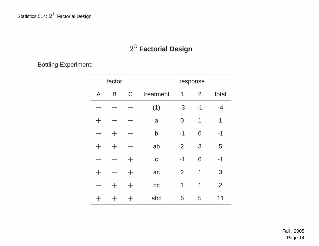
23 Factorial Design
Bottling Experiment:
factor response
A B C treatment 1 2 total
− − − (1) -3 -1 -4
+ − − a 0 1 1
− + − b -1 0 -1
+ + − ab 2 3 5
− − + c -1 0 -1
+ − + ac 2 1 3
− + + bc 1 1 2
+ + + abc 6 5 11
Fall , 2005Page 14

Statistics 514: 2k Factorial Design
factorial effects and constrasts
Main effects:
A = m.e.(A) = y(A+) − y(A−)
= 14 (y(−−−) + y(+ −−) − y(− + −) + y(+ + −) − y(−− +)
+y(+ − +) − y(− + +) + y(+ + +))=3.00
The contrast is (-1,1,-1,1,-1,1,-1,1)
B : (−1,−1, 1, 1,−1,−1, 1, 1), B = 2.25C : (−1,−1,−1,−1, 1, 1, 1, 1), C = 1.75
2-factor interactions:
AB: A × B componentwise, AB=.75
AC : A × C componentwise, AC=.25
BC : B × C componentwise, BC=.50
Fall , 2005Page 15

Statistics 514: 2k Factorial Design
3-factor interaction:
ABC = int(ABC) =12(int(AB | C+) − int(AB | C−))
= 14 (−y(−−−) + y(+ −−) + y(− + −) − y(+ + −)
+y(−− +) − y(+ − +) − y(− + +) + y(+ + +))=.50
The contrast is (-1,1,1,-1,1,-1,-1,1)= A × B × C .
Fall , 2005Page 16

Statistics 514: 2k Factorial Design
Contrasts for Calculating Effects in 23 Design
factorial effects
A B C treatment I A B AB C AC BC ABC
− − − (1) 1 -1 -1 1 -1 1 1 -1
+ − − a 1 1 -1 -1 -1 -1 1 1
− + − b 1 -1 1 -1 -1 1 -1 -1
+ + − ab 1 1 1 1 -1 -1 -1 1
− − + c 1 -1 -1 1 1 -1 -1 1
+ − + ac 1 1 -1 -1 1 1 -1 -1
− + + bc 1 -1 1 -1 1 -1 1 -1
+ + + abc 1 1 1 1 1 1 1 1
Fall , 2005Page 17

Statistics 514: 2k Factorial Design
Estimates:
grand mean:
∑yi.
23
effect :∑
ciyi.
23−1
Contrast Sum of Squares:
SSeffect =(∑
ciyi.)2
23/n= 2n(effect)2
Variance of Estimate
Var(effect) =σ2
n23−2
t-test for effects (confidence interval approach)
effect ± tα/2,2k(n−1)S.E.(effect)
Fall , 2005Page 18

Statistics 514: 2k Factorial Design
Regresson Model
Code the levels of factor A and B as follows
A x1 B x2 C x3
- -1 - -1 - -1
+ 1 + 1 + 1
Fit regression model
y = β0 + β1x1 + β2x2 + β3x3 + β12x1x2 + β13x1x3 + β23x2x3 + β123x1x2x3 + ε
The fitted model should be
y = y.. +A
2x1 +
B
2x2 +
C
2x3 +
AB
2x1x2 +
AC
2x1x3 +
BC
2x2x3 +
ABC
2x1x2x3
i.e. β = effect2
, and
Var(β) =σ2
n2k=
σ2
n23
Fall , 2005Page 19

Statistics 514: 2k Factorial Design
SAS Code: Bottling Experiment
data bottle;
input A B C devi;
datalines;
-1 -1 -1 -3
-1 -1 -1 -1
1 -1 -1 0
1 -1 -1 1
-1 1 -1 -1
-1 1 -1 0
1 1 -1 2
1 1 -1 3
-1 -1 1 -1
-1 -1 1 0
1 -1 1 2
1 -1 1 1
-1 1 1 1
-1 1 1 1
1 1 1 6
1 1 1 5
Fall , 2005Page 20

Statistics 514: 2k Factorial Design
;
proc glm;
class A B C; model devi=A|B|C;
output out=botone r=res p=pred;
run;
proc univariate data=botone pctldef=4;
var res; qqplot res / normal (L=1 mu=est sigma=est);
histogram res / normal; run;
proc gplot; plot res*pred/frame; run;
data bottlenew;
set bottle;
x1=A; x2=B; x3=C; x1x2=x1*x2; x1x3=x1*x3; x2x3=x2*x3;
x1x2x3=x1*x2*x3; drop A B C;
proc reg data=bottlenew;
model devi=x1 x2 x3 x1x2 x1x3 x2x3 x1x2x3;
Fall , 2005Page 21

Statistics 514: 2k Factorial Design
SAS output for Bottling Experiment
ANOVA Model:
Dependent Variable: devi
Sum of
Source DF Squares Mean Square F Value Pr > F
Model 7 73.00000000 10.42857143 16.69 0.0003
Error 8 5.00000000 0.62500000
CorTotal 15 78.00000000
A 1 36.00000000 36.00000000 57.60 <.0001
B 1 20.25000000 20.25000000 32.40 0.0005
A*B 1 2.25000000 2.25000000 3.60 0.0943
C 1 12.25000000 12.25000000 19.60 0.0022
A*C 1 0.25000000 0.25000000 0.40 0.5447
B*C 1 1.00000000 1.00000000 1.60 0.2415
A*B*C 1 1.00000000 1.00000000 1.60 0.2415
Fall , 2005Page 22

Statistics 514: 2k Factorial Design
Regression Model:
Parameter Standard
Variable DF Estimate Error t Value Pr > |t|
Intercept 1 1.00000 0.19764 5.06 0.0010
x1 1 1.50000 0.19764 7.59 <.0001
x2 1 1.12500 0.19764 5.69 0.0005
x3 1 0.87500 0.19764 4.43 0.0022
x1x2 1 0.37500 0.19764 1.90 0.0943
x1x3 1 0.12500 0.19764 0.63 0.5447
x2x3 1 0.25000 0.19764 1.26 0.2415
x1x2x3 1 0.25000 0.19764 1.26 0.2415
Fall , 2005Page 23

Statistics 514: 2k Factorial Design
General 2k Design
• k factors: A, B, . . . , K each with 2 levels (+,−)
• consists of all possible level combinations (2k treatments) each with n replicates
• Classify factorial effects:
type of effect label the number of effects
main effects (of order 1) A, B, C , . . . , K k
2-factor interactions (of order 2) AB, AC , . . . , JK
k
2
3-factor interactions (of order 3) ABC ,ABD,. . . ,IJK
k
3
. . . . . . . . .
k-factor interaction (of order k) ABC · · ·K k
k
Fall , 2005Page 24

Statistics 514: 2k Factorial Design
• In total, how many effects?
• Each effect (main or interaction) has 1 degree of freedom
full model (i.e. model consisting of all the effects) has 2k − 1 degrees of
freedom.
• Error component has 2k(n − 1) degrees of freedom (why?).
• One-to-one correspondence between effects and contrasts:
– For main effect: convert the level column of a factor using − ⇒ −1 and
+ ⇒ 1
– For interactions: multiply the contrasts of the main effects of the involved
factors, componentwisely.
Fall , 2005Page 25

Statistics 514: 2k Factorial Design
General 2k Design: Analysis
• Estimates:
grand mean :
∑yi
2k
For effect with constrast C = (c1, c2, . . . , c2k ), its estimate is
effect =
∑ciyi
2(k−1)
• Variance
Var(effect) =σ2
n2k−2
what is the standard error of the effect?
• t-test for H0: effect=0. Using the confidence interval approach,
effect ± tα/2,2k(n−1)S.E.(effect)
Fall , 2005Page 26

Statistics 514: 2k Factorial Design
Using ANOVA model :
• Sum of Squares due to an effect, using its constrast,
SSeffect =
∑ciy
2i.
2k/n= n2k−2(effect)2
• SST and SSE can be calculated as before and a ANOVA table including SS due to
the effests and SSE can be constructed and the effects can be tested by F -tests.
Using regression :
• Introducing variables x1, . . . , xk for main effects, their products are used for
interactsions, the following regression model can be fitted
y = β0 + β1x1 + . . . + βkxk + . . . + β12···kx1x2 · · ·xk + ε
The coefficients are estimated by half of effects they represent, that is,
β =effect
2
Fall , 2005Page 27

Statistics 514: 2k Factorial Design
Unreplicated 2k Design
Filtration Rate Experiment
Fall , 2005Page 28

Statistics 514: 2k Factorial Design
factor
A B C D filtration
− − − − 45
+ − − − 71
− + − − 48
+ + − − 65
− − + − 68
+ − + − 60
− + + − 80
+ + + − 65
− − − + 43
+ − − + 100
− + − + 45
+ + − + 104
− − + + 75
+ − + + 86
− + + + 70
+ + + + 96
Fall , 2005Page 29

Statistics 514: 2k Factorial Design
Unreplicated 2k Design
• No degree of freedom left for error component if full model is fitted.
• Formulas used for estimates and contrast sum of squares are given in Slides
26-27 with n=1
• No error sum of squares available, cannot estimate σ2 and test effects in both
the ANOVA and Regression approaches.
• Approach 1 : pooling high-order interactions
– Often assume 3 or higher interactions do not occur
– Pool estimates together for error
– Warning: may pool significant interaction
Fall , 2005Page 30

Statistics 514: 2k Factorial Design
Unreplicated 2k Design
• Approach 2: Using the normal probability plot (QQ plot) to identify significant
effects.
– Recall
Var(effect) =σ2
2(k−2)
If the effect is not significant (=0), then the effect estimate follows
N(0, σ2
2(k−2) )
– Assume all effects not significant, their estimates can be considered as a
random sample from N(0, σ2
2(k−2) )
– QQ plot of the estimates is expected to be a linear line
– Deviation from a linear line indicates significant effects
Fall , 2005Page 31

Statistics 514: 2k Factorial Design
Using SAS to generate QQ plot for effects
goption colors=(none);
data filter;
do D = -1 to 1 by 2;do C = -1 to 1 by 2;
do B = -1 to 1 by 2;do A = -1 to 1 by 2;
input y @@; output;
end; end; end; end;
datalines;
45 71 48 65 68 60 80 65 43 100 45 104 75 86 70 96
;
data inter; /* Define Interaction Terms */
set filter;
AB=A*B; AC=A*C; AD=A*D; BC=B*C; BD=B*D; CD=C*D; ABC=AB*C; ABD=AB*D;
ACD=AC*D; BCD=BC*D; ABCD=ABC*D;
proc glm data=inter; /* GLM Proc to Obtain Effects */
class A B C D AB AC AD BC BD CD ABC ABD ACD BCDABCD;
model y=A B C D AB AC AD BC BD CD ABC ABD ACD BCDABCD;
Fall , 2005Page 32

Statistics 514: 2k Factorial Design
estimate ’A’ A 1 -1; estimate ’AC’ AC 1 -1;
run;
proc reg outest=effects data=inter; /* REG Proc to Obtain Effects */
model y=A B C D AB AC AD BC BD CD ABC ABD ACD BCDABCD;
data effect2; set effects;
drop y intercept _RMSE_;
proc transpose data=effect2 out=effect3;
data effect4; set effect3; effect=col1*2;
proc sort data=effect4; by effect;
proc print data=effect4;
/*Generate the QQ plot */
proc rank data=effect4 out=effect5 normal=blom;
var effect; ranks neff;
proc print data=effect5;
symbol1 v=circle;
proc gplot data=effect5;
plot effect*neff=_NAME_;
run;
Fall , 2005Page 33

Statistics 514: 2k Factorial Design
Ranked Effects
Obs _NAME_ COL1 effect neff
1 AC -9.0625 -18.125 -1.73938
2 BCD -1.3125 -2.625 -1.24505
3 ACD -0.812data filter;
do D = -1 to 1 by 2;do C = -1 to 1 by 2;
do B = -1 to 1 by 2;do A = -1 to 1 by 2;
input y @@; output;
end; end; end; end;
datalines;
45 71 48 65 68 60 80 65 43 100 45 104 75 86 70 96
;5 -1.625 -0.94578
4 CD -0.5625 -1.125 -0.71370
5 BD -0.1875 -0.375 -0.51499
6 AB 0.0625 0.125 -0.33489
7 ABCD 0.6875 1.375 -0.16512
8 ABC 0.9375 1.875 -0.00000
9 BC 1.1875 2.375 0.16512
Fall , 2005Page 34

Statistics 514: 2k Factorial Design
10 B 1.5625 3.125 0.33489
11 ABD 2.0625 4.125 0.51499
12 C 4.9375 9.875 0.71370
13 D 7.3125 14.625 0.94578
14 AD 8.3125 16.625 1.24505
15 A 10.8125 21.625 1.73938
Fall , 2005Page 35

Statistics 514: 2k Factorial Design
QQ plot
Fall , 2005Page 36

Statistics 514: 2k Factorial Design
Filtration Experiment Analysis
Fit a linear line based on small effects, identify the effects which are potentially
significant, then use ANOVA or regression fit a sub-model with those effects.
1. Potentially significant effects: A, AD, C, D, AC .
2. Use main effect plot and interaction plot
3. ANOVA model involving only A, C , D and their interactions (projecting the
original unreplicated 24 experiment onto a replicated 23 experiement)
4. regression model only involving A, C , D, AC and AD.
5. Diagnostics using residuals.
Fall , 2005Page 37

Statistics 514: 2k Factorial Design
Interaction Plots for AC and AD
* data step is the same.
proc sort; by A C;
proc means noprint;
var y; by A C;
output out=ymeanac mean=mn;
symbol1 v=circle i=join; symbol2 v=square i=join;
proc gplot data=ymeanac; plot mn*A=C;
run;
* similar code for AD interaction plot
Fall , 2005Page 38

Statistics 514: 2k Factorial Design
Fall , 2005Page 39

Statistics 514: 2k Factorial Design
Fall , 2005Page 40

Statistics 514: 2k Factorial Design
ANOVA with A, C and D and their interactions
proc glm data=filter;
class A C D;
model y=A|C|D;
==================================
Source DF Sum Squares Mean Square F Value Pr > F
Model 7 5551.437500 793.062500 35.35 <.0001
Error 8 179.500000 22.437500
Cor Total 15 5730.937500
Source DF Type I SS Mean Square F Value Pr > F
A 1 1870.562500 1870.562500 83.37 <.0001
C 1 390.062500 390.062500 17.38 0.0031
A*C 1 1314.062500 1314.062500 58.57 <.0001
D 1 855.562500 855.562500 38.13 0.0003
A*D 1 1105.562500 1105.562500 49.27 0.0001
C*D 1 5.062500 5.062500 0.23 0.6475
A*C*D 1 10.562500 10.562500 0.47 0.5120
*ANOVA confirms that A, C, D, AC and AD are significant effects
Fall , 2005Page 41
Statistics 514: 2k Factorial Design
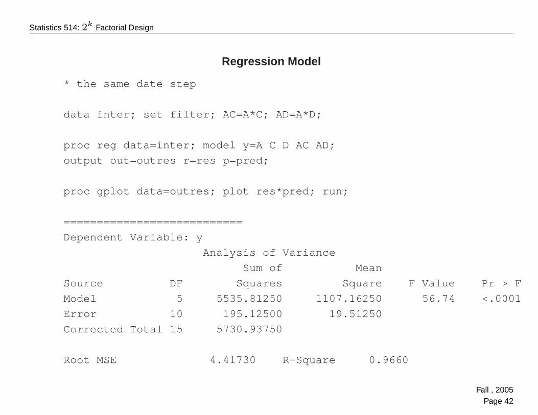
Regression Model
* the same date step
data inter; set filter; AC=A*C; AD=A*D;
proc reg data=inter; model y=A C D AC AD;
output out=outres r=res p=pred;
proc gplot data=outres; plot res*pred; run;
===========================
Dependent Variable: y
Analysis of Variance
Sum of Mean
Source DF Squares Square F Value Pr > F
Model 5 5535.81250 1107.16250 56.74 <.0001
Error 10 195.12500 19.51250
Corrected Total 15 5730.93750
Root MSE 4.41730 R-Square 0.9660
Fall , 2005Page 42

Statistics 514: 2k Factorial Design
Dependent Mean 70.06250 Adj R-Sq 0.9489
Coeff Var 6.30479
Parameter Estimates
Parameter Standard
Variable DF Estimate Error t Value Pr > |t|
Intercept 1 70.06250 1.10432 63.44 <.0001
A 1 10.81250 1.10432 9.79 <.0001
C 1 4.93750 1.10432 4.47 0.0012
D 1 7.31250 1.10432 6.62 <.0001
AC 1 -9.06250 1.10432 -8.21 <.0001
AD 1 8.31250 1.10432 7.53 <.0001
Fall , 2005Page 43
Statistics 514: 2k Factorial Design
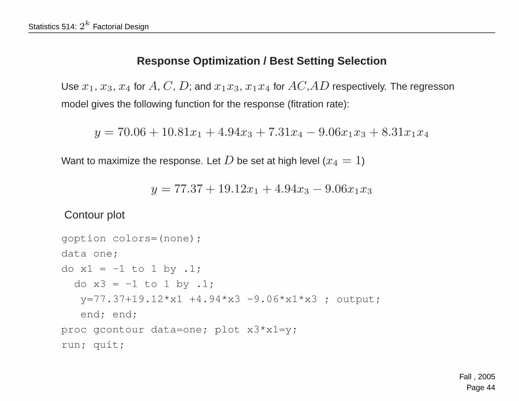
Response Optimization / Best Setting Selection
Use x1, x3, x4 for A, C , D; and x1x3, x1x4 for AC ,AD respectively. The regresson
model gives the following function for the response (fitration rate):
y = 70.06 + 10.81x1 + 4.94x3 + 7.31x4 − 9.06x1x3 + 8.31x1x4
Want to maximize the response. Let D be set at high level (x4 = 1)
y = 77.37 + 19.12x1 + 4.94x3 − 9.06x1x3
Contour plot
goption colors=(none);
data one;
do x1 = -1 to 1 by .1;
do x3 = -1 to 1 by .1;
y=77.37+19.12*x1 +4.94*x3 -9.06*x1*x3 ; output;
end; end;
proc gcontour data=one; plot x3*x1=y;
run; quit;
Fall , 2005Page 44

Statistics 514: 2k Factorial Design
Contour Plot for Response Given D
Fall , 2005Page 45

Statistics 514: 2k Factorial Design
Residual Plot
Fall , 2005Page 46

Statistics 514: 2k Factorial Design
Some Other Issues
• Half normal plot for (xi), i = 1, . . . , n:
– let xi be the absolute values of xi
– sort the (xi): x(1) ≤ ... ≤ x(n)
– calculate ui = Φ−1( n+i2n+1 ), i = 1, ..., n
– plot x(i) against ui
– look for a straight line
Half normal plot can also be used for identifying important factorial effects
• Other methods to identify significant factorial effects (Lenth method).
Hamada&Balakrishnan (1998) analyzing unreplicated factorial experiments: a
review with some new proposals, statistica sinica.
• Detect dispersion effects
• Experiment with duplicate measurements
– for each treatment combination: n responses from duplicate
Fall , 2005Page 47

Statistics 514: 2k Factorial Design
measurements
– calculate mean y and standard deviation s.
– Use y and treat the experiment as unreplicated in analysis
Fall , 2005Page 48

![1 1 1 1 1 1 1 ¢ 1 1 1 - pdfs.semanticscholar.org€¦ · 1 1 1 [ v . ] v 1 1 ¢ 1 1 1 1 ý y þ ï 1 1 1 ð 1 1 1 1 1 x](https://img.pdfslide.us/doc/110x75/5f7bc722cb31ab243d422a20/1-1-1-1-1-1-1-1-1-1-pdfs-1-1-1-v-v-1-1-1-1-1-1-y-1-1-1-.jpg)


![[XLS] · Web view1 1 1 2 3 1 1 2 2 1 1 1 1 1 1 2 1 1 1 1 1 1 2 1 1 1 1 2 2 3 5 1 1 1 1 34 1 1 1 1 1 1 1 1 1 1 240 2 1 1 1 1 1 2 1 3 1 1 2 1 2 5 1 1 1 1 8 1 1 2 1 1 1 1 2 2 1 1 1 1](https://img.pdfslide.us/doc/110x75/5ad1d2817f8b9a05208bfb6d/xls-view1-1-1-2-3-1-1-2-2-1-1-1-1-1-1-2-1-1-1-1-1-1-2-1-1-1-1-2-2-3-5-1-1-1-1.jpg)