Embed Size (px)
Citation preview
Lecture notes 10 Nonlinear Dynamics YFX1520
Lecture 10 1-D maps Lorenz map Logistic map sine mapperiod doubling bifurcation tangent bifurcation tran-sient and intermittent chaos in maps orbit diagram (orFeigenbaum diagram) Feigenbaum constants universalsof unimodal maps universal route to chaos
Contents
1 Lorenz map 211 Cobweb diagram 212 Comparison of fixed point xlowast in 1-D continuous systems and 1-D maps 313 Period-p orbit and stability of period-p points 4
2 1-D maps a proper introduction 5
3 Logistic map 631 Lyapunov exponent 732 Bifurcation analysis and period doubling bifurcation 833 Orbit diagram 1234 Tangent bifurcation and odd number period-p points 13
4 Sine map and universality of period doubling 15
5 Universal route to chaos 16
Handout Orbit diagram of Logistic map
D Kartofelev 117 1003211 As of March 7 2020
Lecture notes 10 Nonlinear Dynamics YFX1520
1 Lorenz map
In this lecture we continue to study the possibility that the Lorenz attractor might be long-termperiodic As in previous lecture we use one-dimensional Lorenz map in the form
zn+1 = f(zn) (1)
to gain insight into the continuous time three-dimensional flow of Lorenz attractor
11 Cobweb diagram
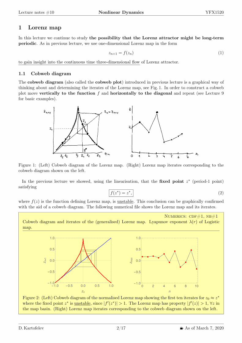
The cobweb diagram (also called the cobweb plot) introduced in previous lecture is a graphical way ofthinking about and determining the iterates of the Lorenz map see Fig 1 In order to construct a cobwebplot move vertically to the function f and horizontally to the diagonal and repeat (see Lecture 9for basic examples)
Figure 1 (Left) Cobweb diagram of the Lorenz map (Right) Lorenz map iterates corresponding to thecobweb diagram shown on the left
In the previous lecture we showed using the linearisation that the fixed point zlowast (period-1 point)satisfying
f(zlowast) = zlowast (2)
where f(z) is the function defining Lorenz map is unstable This conclusion can be graphically confirmedwith the aid of a cobweb diagram The following numerical file shows the Lorenz map and its iterates
Numerics cdf1 nb1Cobweb diagram and iterates of the (generalised) Lorenz map Lyapunov exponent λ(r) of Logisticmap
-10 -05 00 05 10-10
-05
00
05
10
zn
zn+1
0 2 4 6 8 10-10
-05
00
05
10
n
zm
ax
Figure 2 (Left) Cobweb diagram of the normalised Lorenz map showing the first ten iterates for z0 asymp zlowast
where the fixed point zlowast is unstable since |f prime(zlowast)| gt 1 The Lorenz map has property |f prime(z)| gt 1 forallz inthe map basin (Right) Lorenz map iterates corresponding to the cobweb diagram shown on the left
D Kartofelev 217 1003211 As of March 7 2020
Lecture notes 10 Nonlinear Dynamics YFX1520
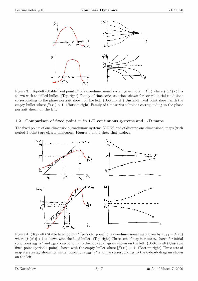
Figure 3 (Top-left) Stable fixed point xlowast of a one-dimensional system given by x = f(x) where f prime(xlowast) lt 1 isshown with the filled bullet (Top-right) Family of time-series solutions shown for several initial conditionscorresponding to the phase portrait shown on the left (Bottom-left) Unstable fixed point shown with theempty bullet where f prime(xlowast) gt 1 (Bottom-right) Family of time-series solutions corresponding to the phaseportrait shown on the left
12 Comparison of fixed point xlowast in 1-D continuous systems and 1-D maps
The fixed points of one-dimensional continuous systems (ODEs) and of discrete one-dimensional maps (withperiod-1 point) are clearly analogous Figures 3 and 4 show that analogy
Figure 4 (Top-left) Stable fixed point xlowast (period-1 point) of a one-dimensional map given by xn+1 = f(xn)where |f prime(xlowast)| lt 1 is shown with the filled bullet (Top-right) Three sets of map iterates xn shown for initialconditions x01 xlowast and x02 corresponding to the cobweb diagram shown on the left (Bottom-left) Unstablefixed point (period-1 point) shown with the empty bullet where |f prime(xlowast)| gt 1 (Bottom-right) Three sets ofmap iterates xn shown for initial conditions x01 xlowast and x02 corresponding to the cobweb diagram shownon the left
D Kartofelev 317 1003211 As of March 7 2020
Lecture notes 10 Nonlinear Dynamics YFX1520
13 Period-p orbit and stability of period-p points
We ended the previous lecture with two open ended questions Can trajectories in the cobweb diagram ofthe Lorenz map close onto themselves And how does a closed trajectory in the cobweb plot translate intothe three-dimensional continuous time Lorenz flow
Figure 5 (Left) Period-4 orbit shown with the red graph where zn+4 = zn (Right) Lorenz map iterateszn corresponding to the cobweb diagram shown on the left Map iterates are repeat every four iterates
So can trajectories in the cobweb diagram of the Lorenz map close onto themselves We could imaginea trajectory of Lorenz maprsquos cobweb plot closing onto itself in a manner shown in Fig 5 Visual inspectionof the cobweb diagram shown in Fig 5 reveals that the iterates zn (local maxima of the three-dimensionalLorenz flow) repeat themselves such that z5 = z1 or more generally
zn+4 = zn foralln (3)
if this dynamics can be shown to be possible then it would strongly suggest that a limit-cycle might bepossible in the three-dimensional Lorenz attractor This conclusion can be generalised further
zn+p = zn foralln (4)
where p isin Z+ is the period of the limit-cycle This type of fixed point is called the period-p point andit represents the period-p orbit of the map The period-p points are a new type of fixed pointsThe period-1 point coincides with our old friendmdashfixed point zlowast The period-p points where p gt 1donrsquot have corresponding analogies in one-dimensional continuous systems in the manner as was discussedin Sec 12 This is because the period-p points represent oscillatory limit-cycle solutions which are notpossible in one-dimensional systems (see Lecture 2 Impossibility of oscillations in 1-D systems)
It is natural to assume that period-p points or orbits very much like fixed points zlowast (period-1 point) canbe either stable (attracting trajectories) or unstable (repelling trajectories) If we can show thatstable period-p orbits are possible in Lorenz map then that would strongly suggest a possibility of periodicsolutions in the continuous time Lorenz attractor
Letrsquos find the analytical expression for the relationship between zn+p and zn in (4) The n+ 1 iterate ofz0 is
zn+1 = f(f(f( f(z0)983167 983166983165 983168n times
))) equiv fn(z0) (5)
The subsequent iterates of the closed period-p orbits similar to the one shown in Fig 5 with the redtrajectory expressed analytically are
(z1 = f(z0))
z2 = f(z1) equiv f1(z1)
z3 = f(z2) = f(f(z1)) equiv f2(z1)
z4 = f(z3) = f(f(f(z1))) equiv f3(z1)
zn+p = fp(zn)
(6)
D Kartofelev 417 1003211 As of March 7 2020
Lecture notes 10 Nonlinear Dynamics YFX1520
where z is the period-p point in the period-p orbit and fp is the pth iterate mapDefinition z is a period-p point if equation
fp(z) = z (7)
where p is minimal is satisfiedThe stability of the period-p point is determined via linearisation For simplicity we consider stability of
period-2 pointf2(z) equiv f(f(z)) = z (8)
Note that z is the period-2 point for map f but the fixed point (period-1) for map f2 In the previous lec-ture we showed that the stability of fixed point zlowast depends on the slope of the map at that point Smallperturbations |η| ≪ 1 evolve according to
ηn+1 asymp |f prime(zlowast)|ηn (9)
We find
|(f2(z))prime| = d
dz|f(f(z))| =
983093
983097983097983097983097983095
chain rule+
orbit pointszn+2 = znwe select z1
983094
983098983098983098983098983096= |f prime(f(z1)983167 983166983165 983168
z2
) middot f prime(z1)| = |f prime(z2)| middot |f prime(z1)| gt 1 (10)
because for the Lorenz map |f prime(z)| gt 1 forallz in the map basin The period-2 point is thus unstable Theevolution of perturbations defined by (9) generalised to all period-p points in any closed period-p orbit arethe following
ηn+p asymp
983055983055983055983055983055
pminus1983132
k=0
f prime(zn+k)
983055983055983055983055983055 ηn (11)
here again by the Lorenz map property983055983055983055983055983055
pminus1983132
k=0
f prime(zn+k)
983055983055983055983055983055 gt 1 (12)
Thus all period-p points are unstable The above analysis of the Lorenz map has strongly demonstrated(not proven) that periodic solutions of Lorenz system are not possible and that the flow is indeed long-term aperiodic for t rarr infin
2 1-D maps a proper introduction
This section deals with a new class of dynamical systems (introduced in Lecture 9) in which time is dis-crete rather than continuous These systems are known variously as difference equations recursionrelations iterated maps or simply maps The Lorenz map is such a system When we say ldquomaprdquo dowe mean the function f or the difference equation
xn+1 = f(xn) (13)
Following common usage wersquoll call both of them maps If yoursquore disturbed by this you must be a puremathematician or should consider becoming one Fixed point xlowast of one-dimensional map (13) satisfiesEq (2) and period-p point x satisfies Eq (7) for minimal p
Maps arise in various ways1 As tools for analysing differential equations We have already encountered maps in this role
For instance Lorenz map provided strong evidence that Lorenz attractor is truly strange and is notjust a long-period limit-cycle In future lectures Poincareacute maps will allowed us to prove the existenceof a periodic solutions and to analyse the stability of periodic solutions in general Maps will proveto be superb tools for studying and analysing chaotic systems
D Kartofelev 517 1003211 As of March 7 2020
Lecture notes 10 Nonlinear Dynamics YFX1520
2 As models of natural phenomena In some scientific contexts it is natural to regard time asdiscrete This is the case in digital electronics in parts of economics and finance theory in impulsivelydriven mechanical systems and in the study of certain animal populations where successive generationsdo not overlap
3 As simple examples of chaos Maps are interesting to study in their own right as mathematicallaboratories for chaos Indeed maps are capable of much wilder behaviour than differential equationsbecause the points xn hop along their orbitstrajectoriesiterates rather than flow continuously Con-tinuity is very much a restriction on possible dynamics (see Lecture 6 Poincareacute-Bendixson theorem)
3 Logistic map
xn+1 = xn
Figure 6 Logistic map and the diagonal
In a fascinating and influential review article (linked below) Robert May (1976) emphasised that evensimple nonlinear maps could have very complicated dynamics May illustrated his point with the Logisticmap given by
xn+1 = rxn(1minus xn) (14)
a discrete-time analog of the Logistic equation for population growth where xn is the dimensionless mea-sure of the population in the nth generation and r is the intrinsic growth rate As shown in Fig 6 the graphof map (14) is a parabola with a maximum value of r4 at x = 12 We restrict the control parameter r tothe range (minus2 or) 0 le r le 4 so that Eq (14) maps the interval 0 le x le 1 into itself
Slide 3Logistic map
Logistic map1 has the form
xn+1 = rxn(1 xn) x0 2 [0 1] r 2 [0 4] n 2 Z+ (1)
where r is the control parameter
Read Robert M May ldquoSimple mathematical models with verycomplicated dynamicsrdquo Nature 261 pp 459ndash467 1976doi101038261459a0
1See Mathematica nb file (cobweb diagram and orbit diagram) uploaded tothe course webpage
DKartofelev YFX1520 3 18
Reading suggestion
Link File name CitationPaper1 paper2pdf Robert M May ldquoSimple mathematical models with very complicated dynam-
icsrdquo Nature 261 pp 459ndash467 (1976)doi101038261459a0
D Kartofelev 617 1003211 As of March 7 2020
Lecture notes 10 Nonlinear Dynamics YFX1520
31 Lyapunov exponent
The calculation of Lyapunov exponents of differential equations is not a trivial task In the case of maps itis much easier We remind that the positive Lyapunov exponent λ is a sign of chaos
Slides 4ndash6
Lyapunov exponent of Logistic map
Chaos is characterised by sensitive dependence on initialconditions If we take two close-by initial conditions say x0 andy0 = x0 + with 1 and iterate them under the map then thedicrarrerence between the two time series n = yn xn should growexponentially
|n| |0en| (2)
where is the Lyapunov exponent For maps this definition leads toa very simple way of measuring Lyapunov exponents Solving (2) for gives
=1
nln
n0
(3)
By definition n = fn(x0 + 0) fn(x0) Thus
=1
nln
fn(x0 + 0) fn(x0)
0
(4)
DKartofelev YFX1520 4 18
Lyapunov exponent of Logistic map
For small values of 0 the quantity inside the absolute value signs isjust the derivative of fn with respect to x evaluated at x = x0
=1
nln
dfn
dx
x=x0
(5)
Since fn(x) = f(f(f( f(x))) ) by the chain ruledfn
dx
x=x0
=f 0(fn1(x0)) middot f 0(fn2(x0)) middot middot f 0(x0)
= |f 0(xn1) middot f 0(xn2) middot middot f 0(x0)| =
n1Y
i=0
f 0(xi)
(6)
Our expression for the Lyapunov exponent becomes
=1
nln
n1Y
i=0
f 0(xi)
=1
n
n1X
i=0
ln |f 0(xi)| (7)
DKartofelev YFX1520 5 18
Lyapunov exponent of Logistic map
=1
nln
n1Y
i=0
f 0(xi)
=1
n
n1X
i=0
ln |f 0(xi)|
Lyapunov exponent is the large iterate n limit of this expression andso we have
= limn1
1
n
n1X
i=0
ln |f 0(xi)| (8)
This formula can be used to study Lyapunov exponent2 as a functionof control parameter r
(r) = limn1
1
n
n1X
i=0
ln |f 0(xi r)| (9)
2See Mathematica nb file uploaded to course webpageDKartofelev YFX1520 6 18
The obtained algorithm is used in the following numerical file to calculate the Lyapunov exponent of theLogistic map as a function of the growth rate r
Numerics cdf1 nb1Cobweb diagram and iterates of the (generalised) Lorenz map Lyapunov exponent λ(r) of the Logisticmap
-2 -1 0 1 2 3 4
-3
-2
-1
0
r
Figure 7 Lyapunov exponent of the Logistic map as a function of the growth rate r Calculation uses5000 iterations for every r value plotted
D Kartofelev 717 1003211 As of March 7 2020
Lecture notes 10 Nonlinear Dynamics YFX1520
32 Bifurcation analysis and period doubling bifurcation
Next letrsquos consider only the stable fixed point and stable period-p points as we incrementally increase thevalue of control parameter r ge 0 We do that in order to simplify our analysis and to save some lecturetime The stable fixed point (period-1 point) of Logistic map given by (14) and satisfying condition (2) is
f(xlowast) = xlowast rArr rxlowast(1minus xlowast) = xlowast | divide xlowast (15)
r(1minus xlowast) = 1 (16)
r minus rxlowast = 1 | divide r (17)
1minus xlowast =1
r (18)
xlowast = 1minus 1
r (19)
Additionally there are the trivial solutions xlowast = 0 and xlowast = 1 (for initial condition x0 = xlowast = 1 and forn gt 1 xn rarr xlowast = 0) Fixed point (19) is stable for |f prime(xlowast)| lt 1 Using map definition (14) we write
|f prime(xlowast)| =983055983055[rx(1minus x)]prime
983055983055x=xlowast = |r minus 2rxlowast| lt 1 (20)
Using condition (20) and for the trivial fixed point xlowast = 0 we get
|r minus 0| lt 1 (21)
|r| lt 1 (22)
The other trivial fixed point xlowast = 1 gives the same result
|r minus 2r| lt 1 (23)
|minus r| lt 1 (24)
Thus the fixed points xlowast = 0 and xlowast = 1 are stable for |plusmnr| lt 1 For the non-trivial fixed point xlowast = 1minus1rand for condition (20) we find 983055983055983055983055r minus 2r
9830611minus 1
r
983062983055983055983055983055 lt 1 (25)
|r minus 2r + 2| lt 1 (26)
|2minus r| lt 1 (27)
1 lt |r| lt 3 (28)
The fixed points xlowast = 1minus 1r exist and is stable for 1 lt |r| lt 3It seems that the found intervals (22) (24) and (28) excluded r = 1 (obviously it does not satisfy
|f prime(xlowast)| lt 1) Letrsquos find the value of the map slope |f prime(xlowast)| for r = 1 using (20) in the case of the trivialsolutions xlowast = 0
|f prime(xlowast)| = |1minus 0| = 1 (29)
xlowast = 1|f prime(xlowast)| = |1minus 2| = 1 (30)
and in the non-trivial case for xlowast = 1minus 1r = 1minus 1 = 0 Which should obviously generate the same result
|f prime(xlowast)| =9830559830559830559830551minus 2
9830611minus 1
1
983062983055983055983055983055 = |1minus 0| = 1 (31)
Below it will also be beneficial to know what happens for r = 3 the r value just after the interval (28)We consider the non-trivial fixed point xlowast = 1minus 1r and find the slope
|f prime(xlowast)| =9830559830559830559830553minus 2 middot 3
9830611minus 1
3
983062983055983055983055983055 = |3minus 4| = |minus 1| = 1 (32)
Usually slope |f prime(xlowast)| = 1 corresponds to the (period doubling or flip) bifurcation point Values r = 1and r = 3 are the bifurcation points Figure 8 shows the map positions of the fixed points and map slopes|f prime(xlowast)| evaluated at the non-trivial fixed point xlowast = 1minus 1r for r = 1 and r = 3
D Kartofelev 817 1003211 As of March 7 2020
Lecture notes 10 Nonlinear Dynamics YFX1520
Figure 8 (Left) Map slope at the fixed points xlowast = 1 minus 1r (same as the trivial case xlowast = 0) for r = 1(Right) Map slope at the fixed points xlowast = 1minus 1r for r = 3
The following interactive numerical file show the dynamics of Logistic map for 0 le |r| lt 1 and 1 lt |r| lt 3
Numerics cdf2 nb2Cobweb diagram of the Logistic map Orbit diagram of the Logistic map Period doubling and orbitdiagram
00 02 04 06 08 1000
02
04
06
08
10
xn
xn+1
0 5 10 15 2000
02
04
06
08
10
n
xn
00 02 04 06 08 1000
02
04
06
08
10
xn
xn+1
0 5 10 15 2000
02
04
06
08
10
n
xn
Figure 9 (Top-left) Cobweb diagram of the Logistic map shown for r = 098 lt 1 The fixed pointxlowast = 0 (Top-right) Map iterates corresponding to the cobweb diagram shown on the left (Bottom-left)Cobweb diagram of the Logistic map shown for interval 1 lt |r| lt 3 with r = 282 The fixed pointxlowast = 1minus 1r (Bottom-right) Map iterates corresponding to the cobweb diagram shown on the left
What happens for r ge 3 What happens after the period doubling or flip bifurcation at r = 3 Thename ldquofliprdquo refers to the fact that the map trajectories start to flip between two values mdash period-2 pointsin period-2 orbit Letrsquos check the dynamics using a computer
Numerics cdf2 nb2Cobweb diagram of the Logistic map Orbit diagram of the Logistic map Period doubling and orbitdiagramAfter the initial transient behaviour has decayed the dynamics of the map settles to a stableperiod-2 orbit It can be showed that period-2 orbits exist for 3 le r lt 1 +
radic6
D Kartofelev 917 1003211 As of March 7 2020
Lecture notes 10 Nonlinear Dynamics YFX1520
00 02 04 06 08 1000
02
04
06
08
10
xn
xn+1
0 5 10 15 20 25 3000
02
04
06
08
10
n
xn
Figure 10 (Left) Cobweb diagram of the Logistic map shown for r = 319 ge 3 featuring the stableperiod-2 point (Right) Map iterates corresponding to the cobweb diagram shown on the left
Letrsquos try to think about this outcome some more
Slides 7ndash9
Logistic map period-2 window
Period-2 window for 3 r lt 1 +p6
Figure Logistic map where r = 318 and x0 = 035 Fixed points (fps)in the case where r lt 3 are shown with the grey bullets Period-2 pointsof f(x) map for r 3 are shown with the blue bullets The fixed points off2(x) map for r 3 are shown with the red bullets
DKartofelev YFX1520 7 18
Logistic map period-2 window
Period-2 window for 3 r lt 1 +p6
(f(p) = rp(1 p) = q
f(q) = rq(1 q) = p(10)
where period-2 point values p and q are the fps of f(x) map
On the other hand it also holds(f(p) = f(f(q)) f 2(q) = r[rq(1 q)][1 (rq(1 q))] = q
f(q) = f(f(p)) f 2(p) = r[rp(1 p)][1 (rp(1 p))] = p)
(11)) f 2(x) = r[rx(1 x)][1 (rx(1 x))] = x (12)
where period-2 point values p and q are the fps of f 2(x) map
DKartofelev YFX1520 8 18
If you want to study the dynamics of the attractors of second iterate map f2 analytically consider oneof the equations in (11 slide numbering) The fourth order polynomial defined by Eq (7)
r[rx(1minus x)][1minus (rx(1minus x))] = x (33)
minus r3x4 + 2r3x3 minus r2(1 + r)x2 + r2x = x (34)
Intersections between the graph of second iterate map f2 and the diagonal correspond to the solutionsof f2(x) = x (34)
Stability of fps of f 2map in period-2 orbit
We need to know the slopes of period-2 points(f(p) = rp(1 p) = q
f(q) = rq(1 q) = p
According to the chain rule it holds that
(f 2(x))0 (f(f(x))0 = f 0(f(x)) middot f 0(x) (13)
In our case
(f 2(p))0 = f 0(f(p)) middot f 0(p) = f 0(q) middot f 0(p)
(f 2(q))0 = f 0(f(q)) middot f 0(q) = f 0(p) middot f 0(q)
)) (f 2(p))0 = (f 2(q))0
(14)Above follows from the commutative property of multiplication
DKartofelev YFX1520 9 18
D Kartofelev 1017 1003211 As of March 7 2020
Lecture notes 10 Nonlinear Dynamics YFX1520
The slopes of map f2 at its fixed points p and q are equal and they are the products of map f slopesat its respective period-2 points
What happens for r ge 1 +radic6 Once again we use a computer
Numerics cdf2 nb2Cobweb diagram of the Logistic map Orbit diagram of the Logistic map Period doubling and orbitdiagram
A period-4 orbit has emerged It can be shown that period-4 orbits exist for 1 +radic6 le r lt 354409
00 02 04 06 08 1000
02
04
06
08
10
xn
xn+1
0 5 10 15 20 25 3000
02
04
06
08
10
n
xn
Figure 11 (Left) Cobweb diagram of the Logistic map shown for r = 3535 ge 1 +radic6 featuring the
stable period-4 point The blue graph shows fourth iterate map f4 (Right) Map iterates correspondingto the cobweb diagram of map f shown on the left
Figure 12 counts the period-4 pointsiterates in the period-4 orbit of the Logistic map Compare Fig 12 toFig 5
Figure 12 Period-4 orbit in the Logistic map
What have we seen so far As we have incrementally increased the value of control parameter r theperiods of the fixed points have increased as well mdash from period-1 to period-2 and finally to period-4The period is clearly doubling This type of bifurcation is called the period doubling bifurca-tion Further period-doublings to orbits of period-8 -16 -32 etc occur as r increases Specifically letrn denote the value of r where a stable 2n-orbit first appears Then computer experiments reveal that
D Kartofelev 1117 1003211 As of March 7 2020
Lecture notes 10 Nonlinear Dynamics YFX1520
Slide 10
Logistic map period doubling
Even number periods
rn ndash bifurcation point onset of stable period-2n orbit
r1 = 30 period-2r2 = 1 +
p6 344949 period-4
r3 354409 period-8r4 356441 period-16r5 356875 period-32r6 356969 period-64
r1 3569946 period-21
r1 ndash onset of chaos (the accumulation point)
= limn1
rn1 rn2
rn rn1 4669201609 (15)
DKartofelev YFX1520 10 18
Note that the successive bifurcations come faster and faster Ultimately the rn converge toa limiting value rinfin The convergence is (essentially) geometric (itrsquos geometric near rinfin) in the limitof large n the distance between successive transitions shrinks by a constant factor of δ This ratio iscalled the Feigenbaum constant After the accumulation point r gt rinfin the dynamics becomeschaotic as wersquoll see below
33 Orbit diagram
The orbit diagram is also called the fig tree diagram (Feigenbaum in German means ldquofig treerdquo) or (in-correctly) the Feigenbaum diagram You might guess that the system would become more and morechaotic for r gt rinfin as r increases but in fact the dynamics are more subtle than that To see the long-termbehaviour for all values of r at once we plot the orbit diagram a special kind of bifurcation diagramOrbit diagram plots the systemrsquos attractor (stable fixed points and stable period-p points) as a function ofcontrol parameter r
To generate the orbit diagram for yourself yoursquoll need to write a computer program with two loops Firstchoose a value of r Then generate an orbit starting from some random initial condition x0 Iterate for 300cycles or so to allow the system to settle down to its eventual stable behaviour Once the transients havedecayed plot many points say x301 x900 above that r Then move to an adjacent value of r and repeateventually sweeping across the whole diagram
The following interactive numerical file shows the orbit diagram for the Logistic map
Numerics cdf2 nb2Cobweb diagram of the Logistic map Orbit diagram of the Logistic map Period doubling and orbitdiagram
The connection between the cobweb diagram orbit diagram and the Lyapunov exponent is shown in theinteractive numerical file linked below
Numerics cdf3 nb3Logistic map cobweb diagram orbit diagram and map iterates Lyapunov exponent
D Kartofelev 1217 1003211 As of March 7 2020
Lecture notes 10 Nonlinear Dynamics YFX1520
Slides 11 12
Orbit diagram and period doubling
DKartofelev YFX1520 11 18
Zooming into the Logistic map self-similarity
No embedded video files in this pdf
DKartofelev YFX1520 12 18
The period doubling is driven by the subsequent flip bifurcations or supercritical pitchforkbifurcations (if we use the nomenclature introduced in Lecture 2) The unstable fixed point andperiod-p points are omitted from the orbit diagram
Feigenbaum diagram shows both stable and unstable fixed points and period-p points or simplydiagram branches (not shown here)
The orbit diagram of the Logistic map features self-similarity In mathematics a self-similarobject is (exactly or) approximately similar to a part of itself ie the whole has the same shape orquality as one or more of its sub-parts
34 Tangent bifurcation and odd number period-p points
Can an odd number period appear in the Logistic map mdash eg period-3 point One of the most intriguingfeatures of the orbit diagram is the occurrence of periodic windows for r gt rinfin The period-3 windowthat occurs for 1 +
radic8 le r le 38415 is the most conspicuous Suddenly against a backdrop of chaos a
stable period-3 orbit appears out of the blueLetrsquos see if we can find the period-3 window of Logistic map using a computer
Numerics cdf2 nb2Cobweb diagram of the Logistic map Orbit diagram of the Logistic map Period doubling and orbitdiagram
The tangent bifurcation is a new type of bifurcation for us that occurs at r = 1 +radic8
00 02 04 06 08 1000
02
04
06
08
10
xn
xn+1
0 5 10 15 20 25 3000
02
04
06
08
10
n
xn
Figure 13 (Left) Period-3 orbit of map f can be found in the period-3 window Here showing thetrajectory for r = 383 (Right) Map iterates corresponding to the cobweb diagram of map f shownon the left
The mechanism responsible for the occurrence of the odd number periods-p points is shown in Fig 14The intersections between the graph of f3 shown in red and the diagonal correspond to solutions of
D Kartofelev 1317 1003211 As of March 7 2020
Lecture notes 10 Nonlinear Dynamics YFX1520
Figure 14 Period-3 orbit can be found in period-3 window of the orbit diagram
f3(x) = x There are eight solutions for r ge 1+radic8 six of interest to us are marked with the blue dots and
two imposters that are not genuine period-3 they are actually fixed points or period-1 points for whichf(xlowast) = xlowast The blue filled dots in Fig 14 correspond to a stable period-3 cycle note that the slope off3(x) is shallow at these points consistent with the stability of the cycle In contrast the slope exceeds 1at the cycle marked by the empty blue dots this period-3 orbit is therefore unstable
Now suppose we decrease r toward the chaotic regime r lt 1+radic8 Then the red graph in Fig 14 changes
shape mdash the hill moves down and the valleys rise up The curve therefore moves towards the diagonalFigure 14 shows that when r = 1 +
radic8 the six blue intersections have merged to form three black filled
period-3 points by becoming tangent to the diagonal At this critical value of r the stable and unstableperiod-3 cycles coalesce and annihilate in a tangent bifurcation This transition defines the beginning ofthe periodic period-3 window
All odd number periods will also undergo the period doubling This means that all number periods [1infin)are eventually represented in the orbit diagram
Figure 14 also explains the self-similarity present in the orbit diagram as shown on Slide 12 for differentscales of magnification The peaks and valley of map f3 are smaller distorted copies of the original mapf Thus the local dynamics of the cobweb trajectories for map f3 must be similar to the dynamics of theoriginal map f
Slide 13
Intermittency3and period-3 window
Transient chaos and intermittency in dynamical systemsTangent bifurcation occurs at r = 1 +
p8 38284 (period-3 orbit)
50 100 150n
02
04
06
08
10xn
Iterates of Logistic map shown for r = 38282 and x0 = 015
3See Mathematica nb file uploaded to course webpageDKartofelev YFX1520 13 18
The dynamics closely related to the tangent bifurcation is intermittency Logistic map exhibitsintermittent chaos for r values just before the period-3 window
D Kartofelev 1417 1003211 As of March 7 2020
Lecture notes 10 Nonlinear Dynamics YFX1520
Numerics cdf4 nb4Period-3 window and intermittency in the Logistic map (iterates xn)
4 Sine map and universality of period doubling
It can be shown that in all unimodal maps same dynamics of period doubling occurs For example weconsider the sine map
Slide 14
Universality of period doubling in unimodal maps
1-D sine map4 The sine map has the form
xn+1 = r sin(xn) x0 2 [0 1] r 2 [0 1] n 2 Z+ (16)
where r is the control parameter
Read Mitchell J Feigenbaum ldquoQuantitative universality for a classof nonlinear transformationsrdquo Journal of Statistical Physics 19(1)pp 25ndash52 1978 doi101007BF01020332
Read Mitchell J Feigenbaum ldquoUniversal behavior in nonlinearsystemsrdquo Physica D Nonlinear Phenomena 7(1ndash3) pp 16ndash391983 doi1010160167-2789(83)90112-4
4See Mathematica nb file (cobweb diagram and orbit diagram) uploaded tothe course webpage
DKartofelev YFX1520 14 18
The graph of the sine map has the same basic shape as the graph of the Logistic map Both curvesare smooth concave down and have a single maximum Such maps are called unimodal
Sine is also a transcendental function opposed to an algebraic function as is the polynomial thatdescribes the Logistic map A transcendental function is an analytic function that does not satisfy apolynomial equation In other words a transcendental function ldquotranscendsrdquo algebra in that it cannotbe expressed in terms of a finite sequence of the algebraic operations of addition multiplication androot extraction
The transcendental nature of the sine map must makes the underlying higher-dimensional physicsrepresented by the sine map fundamentally different from eg the three-dimensional Lorenz flowsampled by Lorenz map
Letrsquos study the dynamics of the sine map using a computer
Numerics cdf5 nb5The sine map iterates cobweb and orbit diagrams (xn isin [0 1])
Numerics cdf6 nb6The sine map iterates cobweb and orbit diagrams (xn isin [minus1 1])
The dynamics is surprisingly similar to the dynamics of the Logistic map Mitchell J Feigenbaumwas first to discover the quantitative laws that are independent of unimodal map functions f Bythat we mean that the algebraic form of f(x) is irrelevant only its overall shape matters
D Kartofelev 1517 1003211 As of March 7 2020
Lecture notes 10 Nonlinear Dynamics YFX1520
Slide 151-D unimodal maps and Feigenbaum constants
= limn1
n1
n= lim
n1
rn1 rn2
rn rn1 4669201609 (17)
crarr = limn1
dn1
dn 2502907875 (18)
DKartofelev YFX1520 15 18
Here xm = max f(x) is the maximum of the map graph The Feigenbaum constants are valid up tothe onset of chaos at rinfin and inside each periodic window for r gt rinfin
In addition to scaling law in control parameter r direction shown earlier Feigenbaum also foundscaling law for the vertical x-direction of the orbit diagram The Feigenbaum constants are uni-versal the same convergence rate appears no matter what unimodal map is iterated They are newmathematical constants as basic to period doubling as π is to circles
Reading suggestion
Link File name CitationPaper2 paper3pdf Mitchell J Feigenbaum ldquoQuantitative universality for a class of nonlinear trans-
formationsrdquo Journal of Statistical Physics 19(1) pp 25ndash52 (1978)doi101007BF01020332
Paper3 paper4pdf Mitchell J Feigenbaum ldquoUniversal behavior in nonlinear systemsrdquo Physica DNonlinear Phenomena 7(1ndash3) pp 16ndash39 (1983)doi1010160167-2789(83)90112-4
5 Universal route to chaos
We showed that the qualitative dynamics of the Logistic and sine maps are identical They both undergoperiod doubling routes to chaos followed by periodic windows interwoven with chaotic bandsEven more remarkably the periodic windows occur in the same order and with the same relative sizes Forinstance the period-3 window is the largest in both cases and the next largest windows preceding it areperiod-5 and period-6 But there are quantitative differences For instance the period doubling bifurcationsoccur later (for greater parameter r value) in the Logistic map and the periodic windows are thinner
Turns out that the onset of chaos via period doubling is predominant in nature and in artificial chaoticsystems Feigenbaum constants have real predictive power in various scientific applications The perioddoubling bifurcation is the ldquorouterdquo taken by nonlinear systems to reach chaotic solution Interm of the bifurcations introduced in Lecture 2 the period doubling bifurcation can also be seen as a seriesof subsequentsucceeding supercritical pitchfork bifurcations see Slide 11
Revision questions
1 What is cobweb diagram2 What is recurrence map or recurrence relation3 What is 1-D map4 How to find fixed points of 1-D maps5 What is Lorenz map
D Kartofelev 1617 1003211 As of March 7 2020
Lecture notes 10 Nonlinear Dynamics YFX1520
6 What is Logistic map7 What is sine map8 What is period doubling9 What is period doubling bifurcation
10 What is tangent bifurcation11 Do odd number periods (period-p orbits) exist in chaotic systems12 Do even number periods (period-p orbits) exist in chaotic systems13 Can maps produce transient chaos14 Can maps produce intermittency15 Can maps produce intermittent chaos16 What is orbit diagram (or Feigenbaum diagram)17 What are Feigenbaum constants
D Kartofelev 1717 1003211 As of March 7 2020
Lecture notes 10 Nonlinear Dynamics YFX1520
1 Lorenz map
In this lecture we continue to study the possibility that the Lorenz attractor might be long-termperiodic As in previous lecture we use one-dimensional Lorenz map in the form
zn+1 = f(zn) (1)
to gain insight into the continuous time three-dimensional flow of Lorenz attractor
11 Cobweb diagram
The cobweb diagram (also called the cobweb plot) introduced in previous lecture is a graphical way ofthinking about and determining the iterates of the Lorenz map see Fig 1 In order to construct a cobwebplot move vertically to the function f and horizontally to the diagonal and repeat (see Lecture 9for basic examples)
Figure 1 (Left) Cobweb diagram of the Lorenz map (Right) Lorenz map iterates corresponding to thecobweb diagram shown on the left
In the previous lecture we showed using the linearisation that the fixed point zlowast (period-1 point)satisfying
f(zlowast) = zlowast (2)
where f(z) is the function defining Lorenz map is unstable This conclusion can be graphically confirmedwith the aid of a cobweb diagram The following numerical file shows the Lorenz map and its iterates
Numerics cdf1 nb1Cobweb diagram and iterates of the (generalised) Lorenz map Lyapunov exponent λ(r) of Logisticmap
-10 -05 00 05 10-10
-05
00
05
10
zn
zn+1
0 2 4 6 8 10-10
-05
00
05
10
n
zm
ax
Figure 2 (Left) Cobweb diagram of the normalised Lorenz map showing the first ten iterates for z0 asymp zlowast
where the fixed point zlowast is unstable since |f prime(zlowast)| gt 1 The Lorenz map has property |f prime(z)| gt 1 forallz inthe map basin (Right) Lorenz map iterates corresponding to the cobweb diagram shown on the left
D Kartofelev 217 1003211 As of March 7 2020
Lecture notes 10 Nonlinear Dynamics YFX1520
Figure 3 (Top-left) Stable fixed point xlowast of a one-dimensional system given by x = f(x) where f prime(xlowast) lt 1 isshown with the filled bullet (Top-right) Family of time-series solutions shown for several initial conditionscorresponding to the phase portrait shown on the left (Bottom-left) Unstable fixed point shown with theempty bullet where f prime(xlowast) gt 1 (Bottom-right) Family of time-series solutions corresponding to the phaseportrait shown on the left
12 Comparison of fixed point xlowast in 1-D continuous systems and 1-D maps
The fixed points of one-dimensional continuous systems (ODEs) and of discrete one-dimensional maps (withperiod-1 point) are clearly analogous Figures 3 and 4 show that analogy
Figure 4 (Top-left) Stable fixed point xlowast (period-1 point) of a one-dimensional map given by xn+1 = f(xn)where |f prime(xlowast)| lt 1 is shown with the filled bullet (Top-right) Three sets of map iterates xn shown for initialconditions x01 xlowast and x02 corresponding to the cobweb diagram shown on the left (Bottom-left) Unstablefixed point (period-1 point) shown with the empty bullet where |f prime(xlowast)| gt 1 (Bottom-right) Three sets ofmap iterates xn shown for initial conditions x01 xlowast and x02 corresponding to the cobweb diagram shownon the left
D Kartofelev 317 1003211 As of March 7 2020
Lecture notes 10 Nonlinear Dynamics YFX1520
13 Period-p orbit and stability of period-p points
We ended the previous lecture with two open ended questions Can trajectories in the cobweb diagram ofthe Lorenz map close onto themselves And how does a closed trajectory in the cobweb plot translate intothe three-dimensional continuous time Lorenz flow
Figure 5 (Left) Period-4 orbit shown with the red graph where zn+4 = zn (Right) Lorenz map iterateszn corresponding to the cobweb diagram shown on the left Map iterates are repeat every four iterates
So can trajectories in the cobweb diagram of the Lorenz map close onto themselves We could imaginea trajectory of Lorenz maprsquos cobweb plot closing onto itself in a manner shown in Fig 5 Visual inspectionof the cobweb diagram shown in Fig 5 reveals that the iterates zn (local maxima of the three-dimensionalLorenz flow) repeat themselves such that z5 = z1 or more generally
zn+4 = zn foralln (3)
if this dynamics can be shown to be possible then it would strongly suggest that a limit-cycle might bepossible in the three-dimensional Lorenz attractor This conclusion can be generalised further
zn+p = zn foralln (4)
where p isin Z+ is the period of the limit-cycle This type of fixed point is called the period-p point andit represents the period-p orbit of the map The period-p points are a new type of fixed pointsThe period-1 point coincides with our old friendmdashfixed point zlowast The period-p points where p gt 1donrsquot have corresponding analogies in one-dimensional continuous systems in the manner as was discussedin Sec 12 This is because the period-p points represent oscillatory limit-cycle solutions which are notpossible in one-dimensional systems (see Lecture 2 Impossibility of oscillations in 1-D systems)
It is natural to assume that period-p points or orbits very much like fixed points zlowast (period-1 point) canbe either stable (attracting trajectories) or unstable (repelling trajectories) If we can show thatstable period-p orbits are possible in Lorenz map then that would strongly suggest a possibility of periodicsolutions in the continuous time Lorenz attractor
Letrsquos find the analytical expression for the relationship between zn+p and zn in (4) The n+ 1 iterate ofz0 is
zn+1 = f(f(f( f(z0)983167 983166983165 983168n times
))) equiv fn(z0) (5)
The subsequent iterates of the closed period-p orbits similar to the one shown in Fig 5 with the redtrajectory expressed analytically are
(z1 = f(z0))
z2 = f(z1) equiv f1(z1)
z3 = f(z2) = f(f(z1)) equiv f2(z1)
z4 = f(z3) = f(f(f(z1))) equiv f3(z1)
zn+p = fp(zn)
(6)
D Kartofelev 417 1003211 As of March 7 2020
Lecture notes 10 Nonlinear Dynamics YFX1520
where z is the period-p point in the period-p orbit and fp is the pth iterate mapDefinition z is a period-p point if equation
fp(z) = z (7)
where p is minimal is satisfiedThe stability of the period-p point is determined via linearisation For simplicity we consider stability of
period-2 pointf2(z) equiv f(f(z)) = z (8)
Note that z is the period-2 point for map f but the fixed point (period-1) for map f2 In the previous lec-ture we showed that the stability of fixed point zlowast depends on the slope of the map at that point Smallperturbations |η| ≪ 1 evolve according to
ηn+1 asymp |f prime(zlowast)|ηn (9)
We find
|(f2(z))prime| = d
dz|f(f(z))| =
983093
983097983097983097983097983095
chain rule+
orbit pointszn+2 = znwe select z1
983094
983098983098983098983098983096= |f prime(f(z1)983167 983166983165 983168
z2
) middot f prime(z1)| = |f prime(z2)| middot |f prime(z1)| gt 1 (10)
because for the Lorenz map |f prime(z)| gt 1 forallz in the map basin The period-2 point is thus unstable Theevolution of perturbations defined by (9) generalised to all period-p points in any closed period-p orbit arethe following
ηn+p asymp
983055983055983055983055983055
pminus1983132
k=0
f prime(zn+k)
983055983055983055983055983055 ηn (11)
here again by the Lorenz map property983055983055983055983055983055
pminus1983132
k=0
f prime(zn+k)
983055983055983055983055983055 gt 1 (12)
Thus all period-p points are unstable The above analysis of the Lorenz map has strongly demonstrated(not proven) that periodic solutions of Lorenz system are not possible and that the flow is indeed long-term aperiodic for t rarr infin
2 1-D maps a proper introduction
This section deals with a new class of dynamical systems (introduced in Lecture 9) in which time is dis-crete rather than continuous These systems are known variously as difference equations recursionrelations iterated maps or simply maps The Lorenz map is such a system When we say ldquomaprdquo dowe mean the function f or the difference equation
xn+1 = f(xn) (13)
Following common usage wersquoll call both of them maps If yoursquore disturbed by this you must be a puremathematician or should consider becoming one Fixed point xlowast of one-dimensional map (13) satisfiesEq (2) and period-p point x satisfies Eq (7) for minimal p
Maps arise in various ways1 As tools for analysing differential equations We have already encountered maps in this role
For instance Lorenz map provided strong evidence that Lorenz attractor is truly strange and is notjust a long-period limit-cycle In future lectures Poincareacute maps will allowed us to prove the existenceof a periodic solutions and to analyse the stability of periodic solutions in general Maps will proveto be superb tools for studying and analysing chaotic systems
D Kartofelev 517 1003211 As of March 7 2020
Lecture notes 10 Nonlinear Dynamics YFX1520
2 As models of natural phenomena In some scientific contexts it is natural to regard time asdiscrete This is the case in digital electronics in parts of economics and finance theory in impulsivelydriven mechanical systems and in the study of certain animal populations where successive generationsdo not overlap
3 As simple examples of chaos Maps are interesting to study in their own right as mathematicallaboratories for chaos Indeed maps are capable of much wilder behaviour than differential equationsbecause the points xn hop along their orbitstrajectoriesiterates rather than flow continuously Con-tinuity is very much a restriction on possible dynamics (see Lecture 6 Poincareacute-Bendixson theorem)
3 Logistic map
xn+1 = xn
Figure 6 Logistic map and the diagonal
In a fascinating and influential review article (linked below) Robert May (1976) emphasised that evensimple nonlinear maps could have very complicated dynamics May illustrated his point with the Logisticmap given by
xn+1 = rxn(1minus xn) (14)
a discrete-time analog of the Logistic equation for population growth where xn is the dimensionless mea-sure of the population in the nth generation and r is the intrinsic growth rate As shown in Fig 6 the graphof map (14) is a parabola with a maximum value of r4 at x = 12 We restrict the control parameter r tothe range (minus2 or) 0 le r le 4 so that Eq (14) maps the interval 0 le x le 1 into itself
Slide 3Logistic map
Logistic map1 has the form
xn+1 = rxn(1 xn) x0 2 [0 1] r 2 [0 4] n 2 Z+ (1)
where r is the control parameter
Read Robert M May ldquoSimple mathematical models with verycomplicated dynamicsrdquo Nature 261 pp 459ndash467 1976doi101038261459a0
1See Mathematica nb file (cobweb diagram and orbit diagram) uploaded tothe course webpage
DKartofelev YFX1520 3 18
Reading suggestion
Link File name CitationPaper1 paper2pdf Robert M May ldquoSimple mathematical models with very complicated dynam-
icsrdquo Nature 261 pp 459ndash467 (1976)doi101038261459a0
D Kartofelev 617 1003211 As of March 7 2020
Lecture notes 10 Nonlinear Dynamics YFX1520
31 Lyapunov exponent
The calculation of Lyapunov exponents of differential equations is not a trivial task In the case of maps itis much easier We remind that the positive Lyapunov exponent λ is a sign of chaos
Slides 4ndash6
Lyapunov exponent of Logistic map
Chaos is characterised by sensitive dependence on initialconditions If we take two close-by initial conditions say x0 andy0 = x0 + with 1 and iterate them under the map then thedicrarrerence between the two time series n = yn xn should growexponentially
|n| |0en| (2)
where is the Lyapunov exponent For maps this definition leads toa very simple way of measuring Lyapunov exponents Solving (2) for gives
=1
nln
n0
(3)
By definition n = fn(x0 + 0) fn(x0) Thus
=1
nln
fn(x0 + 0) fn(x0)
0
(4)
DKartofelev YFX1520 4 18
Lyapunov exponent of Logistic map
For small values of 0 the quantity inside the absolute value signs isjust the derivative of fn with respect to x evaluated at x = x0
=1
nln
dfn
dx
x=x0
(5)
Since fn(x) = f(f(f( f(x))) ) by the chain ruledfn
dx
x=x0
=f 0(fn1(x0)) middot f 0(fn2(x0)) middot middot f 0(x0)
= |f 0(xn1) middot f 0(xn2) middot middot f 0(x0)| =
n1Y
i=0
f 0(xi)
(6)
Our expression for the Lyapunov exponent becomes
=1
nln
n1Y
i=0
f 0(xi)
=1
n
n1X
i=0
ln |f 0(xi)| (7)
DKartofelev YFX1520 5 18
Lyapunov exponent of Logistic map
=1
nln
n1Y
i=0
f 0(xi)
=1
n
n1X
i=0
ln |f 0(xi)|
Lyapunov exponent is the large iterate n limit of this expression andso we have
= limn1
1
n
n1X
i=0
ln |f 0(xi)| (8)
This formula can be used to study Lyapunov exponent2 as a functionof control parameter r
(r) = limn1
1
n
n1X
i=0
ln |f 0(xi r)| (9)
2See Mathematica nb file uploaded to course webpageDKartofelev YFX1520 6 18
The obtained algorithm is used in the following numerical file to calculate the Lyapunov exponent of theLogistic map as a function of the growth rate r
Numerics cdf1 nb1Cobweb diagram and iterates of the (generalised) Lorenz map Lyapunov exponent λ(r) of the Logisticmap
-2 -1 0 1 2 3 4
-3
-2
-1
0
r
Figure 7 Lyapunov exponent of the Logistic map as a function of the growth rate r Calculation uses5000 iterations for every r value plotted
D Kartofelev 717 1003211 As of March 7 2020
Lecture notes 10 Nonlinear Dynamics YFX1520
32 Bifurcation analysis and period doubling bifurcation
Next letrsquos consider only the stable fixed point and stable period-p points as we incrementally increase thevalue of control parameter r ge 0 We do that in order to simplify our analysis and to save some lecturetime The stable fixed point (period-1 point) of Logistic map given by (14) and satisfying condition (2) is
f(xlowast) = xlowast rArr rxlowast(1minus xlowast) = xlowast | divide xlowast (15)
r(1minus xlowast) = 1 (16)
r minus rxlowast = 1 | divide r (17)
1minus xlowast =1
r (18)
xlowast = 1minus 1
r (19)
Additionally there are the trivial solutions xlowast = 0 and xlowast = 1 (for initial condition x0 = xlowast = 1 and forn gt 1 xn rarr xlowast = 0) Fixed point (19) is stable for |f prime(xlowast)| lt 1 Using map definition (14) we write
|f prime(xlowast)| =983055983055[rx(1minus x)]prime
983055983055x=xlowast = |r minus 2rxlowast| lt 1 (20)
Using condition (20) and for the trivial fixed point xlowast = 0 we get
|r minus 0| lt 1 (21)
|r| lt 1 (22)
The other trivial fixed point xlowast = 1 gives the same result
|r minus 2r| lt 1 (23)
|minus r| lt 1 (24)
Thus the fixed points xlowast = 0 and xlowast = 1 are stable for |plusmnr| lt 1 For the non-trivial fixed point xlowast = 1minus1rand for condition (20) we find 983055983055983055983055r minus 2r
9830611minus 1
r
983062983055983055983055983055 lt 1 (25)
|r minus 2r + 2| lt 1 (26)
|2minus r| lt 1 (27)
1 lt |r| lt 3 (28)
The fixed points xlowast = 1minus 1r exist and is stable for 1 lt |r| lt 3It seems that the found intervals (22) (24) and (28) excluded r = 1 (obviously it does not satisfy
|f prime(xlowast)| lt 1) Letrsquos find the value of the map slope |f prime(xlowast)| for r = 1 using (20) in the case of the trivialsolutions xlowast = 0
|f prime(xlowast)| = |1minus 0| = 1 (29)
xlowast = 1|f prime(xlowast)| = |1minus 2| = 1 (30)
and in the non-trivial case for xlowast = 1minus 1r = 1minus 1 = 0 Which should obviously generate the same result
|f prime(xlowast)| =9830559830559830559830551minus 2
9830611minus 1
1
983062983055983055983055983055 = |1minus 0| = 1 (31)
Below it will also be beneficial to know what happens for r = 3 the r value just after the interval (28)We consider the non-trivial fixed point xlowast = 1minus 1r and find the slope
|f prime(xlowast)| =9830559830559830559830553minus 2 middot 3
9830611minus 1
3
983062983055983055983055983055 = |3minus 4| = |minus 1| = 1 (32)
Usually slope |f prime(xlowast)| = 1 corresponds to the (period doubling or flip) bifurcation point Values r = 1and r = 3 are the bifurcation points Figure 8 shows the map positions of the fixed points and map slopes|f prime(xlowast)| evaluated at the non-trivial fixed point xlowast = 1minus 1r for r = 1 and r = 3
D Kartofelev 817 1003211 As of March 7 2020
Lecture notes 10 Nonlinear Dynamics YFX1520
Figure 8 (Left) Map slope at the fixed points xlowast = 1 minus 1r (same as the trivial case xlowast = 0) for r = 1(Right) Map slope at the fixed points xlowast = 1minus 1r for r = 3
The following interactive numerical file show the dynamics of Logistic map for 0 le |r| lt 1 and 1 lt |r| lt 3
Numerics cdf2 nb2Cobweb diagram of the Logistic map Orbit diagram of the Logistic map Period doubling and orbitdiagram
00 02 04 06 08 1000
02
04
06
08
10
xn
xn+1
0 5 10 15 2000
02
04
06
08
10
n
xn
00 02 04 06 08 1000
02
04
06
08
10
xn
xn+1
0 5 10 15 2000
02
04
06
08
10
n
xn
Figure 9 (Top-left) Cobweb diagram of the Logistic map shown for r = 098 lt 1 The fixed pointxlowast = 0 (Top-right) Map iterates corresponding to the cobweb diagram shown on the left (Bottom-left)Cobweb diagram of the Logistic map shown for interval 1 lt |r| lt 3 with r = 282 The fixed pointxlowast = 1minus 1r (Bottom-right) Map iterates corresponding to the cobweb diagram shown on the left
What happens for r ge 3 What happens after the period doubling or flip bifurcation at r = 3 Thename ldquofliprdquo refers to the fact that the map trajectories start to flip between two values mdash period-2 pointsin period-2 orbit Letrsquos check the dynamics using a computer
Numerics cdf2 nb2Cobweb diagram of the Logistic map Orbit diagram of the Logistic map Period doubling and orbitdiagramAfter the initial transient behaviour has decayed the dynamics of the map settles to a stableperiod-2 orbit It can be showed that period-2 orbits exist for 3 le r lt 1 +
radic6
D Kartofelev 917 1003211 As of March 7 2020
Lecture notes 10 Nonlinear Dynamics YFX1520
00 02 04 06 08 1000
02
04
06
08
10
xn
xn+1
0 5 10 15 20 25 3000
02
04
06
08
10
n
xn
Figure 10 (Left) Cobweb diagram of the Logistic map shown for r = 319 ge 3 featuring the stableperiod-2 point (Right) Map iterates corresponding to the cobweb diagram shown on the left
Letrsquos try to think about this outcome some more
Slides 7ndash9
Logistic map period-2 window
Period-2 window for 3 r lt 1 +p6
Figure Logistic map where r = 318 and x0 = 035 Fixed points (fps)in the case where r lt 3 are shown with the grey bullets Period-2 pointsof f(x) map for r 3 are shown with the blue bullets The fixed points off2(x) map for r 3 are shown with the red bullets
DKartofelev YFX1520 7 18
Logistic map period-2 window
Period-2 window for 3 r lt 1 +p6
(f(p) = rp(1 p) = q
f(q) = rq(1 q) = p(10)
where period-2 point values p and q are the fps of f(x) map
On the other hand it also holds(f(p) = f(f(q)) f 2(q) = r[rq(1 q)][1 (rq(1 q))] = q
f(q) = f(f(p)) f 2(p) = r[rp(1 p)][1 (rp(1 p))] = p)
(11)) f 2(x) = r[rx(1 x)][1 (rx(1 x))] = x (12)
where period-2 point values p and q are the fps of f 2(x) map
DKartofelev YFX1520 8 18
If you want to study the dynamics of the attractors of second iterate map f2 analytically consider oneof the equations in (11 slide numbering) The fourth order polynomial defined by Eq (7)
r[rx(1minus x)][1minus (rx(1minus x))] = x (33)
minus r3x4 + 2r3x3 minus r2(1 + r)x2 + r2x = x (34)
Intersections between the graph of second iterate map f2 and the diagonal correspond to the solutionsof f2(x) = x (34)
Stability of fps of f 2map in period-2 orbit
We need to know the slopes of period-2 points(f(p) = rp(1 p) = q
f(q) = rq(1 q) = p
According to the chain rule it holds that
(f 2(x))0 (f(f(x))0 = f 0(f(x)) middot f 0(x) (13)
In our case
(f 2(p))0 = f 0(f(p)) middot f 0(p) = f 0(q) middot f 0(p)
(f 2(q))0 = f 0(f(q)) middot f 0(q) = f 0(p) middot f 0(q)
)) (f 2(p))0 = (f 2(q))0
(14)Above follows from the commutative property of multiplication
DKartofelev YFX1520 9 18
D Kartofelev 1017 1003211 As of March 7 2020
Lecture notes 10 Nonlinear Dynamics YFX1520
The slopes of map f2 at its fixed points p and q are equal and they are the products of map f slopesat its respective period-2 points
What happens for r ge 1 +radic6 Once again we use a computer
Numerics cdf2 nb2Cobweb diagram of the Logistic map Orbit diagram of the Logistic map Period doubling and orbitdiagram
A period-4 orbit has emerged It can be shown that period-4 orbits exist for 1 +radic6 le r lt 354409
00 02 04 06 08 1000
02
04
06
08
10
xn
xn+1
0 5 10 15 20 25 3000
02
04
06
08
10
n
xn
Figure 11 (Left) Cobweb diagram of the Logistic map shown for r = 3535 ge 1 +radic6 featuring the
stable period-4 point The blue graph shows fourth iterate map f4 (Right) Map iterates correspondingto the cobweb diagram of map f shown on the left
Figure 12 counts the period-4 pointsiterates in the period-4 orbit of the Logistic map Compare Fig 12 toFig 5
Figure 12 Period-4 orbit in the Logistic map
What have we seen so far As we have incrementally increased the value of control parameter r theperiods of the fixed points have increased as well mdash from period-1 to period-2 and finally to period-4The period is clearly doubling This type of bifurcation is called the period doubling bifurca-tion Further period-doublings to orbits of period-8 -16 -32 etc occur as r increases Specifically letrn denote the value of r where a stable 2n-orbit first appears Then computer experiments reveal that
D Kartofelev 1117 1003211 As of March 7 2020
Lecture notes 10 Nonlinear Dynamics YFX1520
Slide 10
Logistic map period doubling
Even number periods
rn ndash bifurcation point onset of stable period-2n orbit
r1 = 30 period-2r2 = 1 +
p6 344949 period-4
r3 354409 period-8r4 356441 period-16r5 356875 period-32r6 356969 period-64
r1 3569946 period-21
r1 ndash onset of chaos (the accumulation point)
= limn1
rn1 rn2
rn rn1 4669201609 (15)
DKartofelev YFX1520 10 18
Note that the successive bifurcations come faster and faster Ultimately the rn converge toa limiting value rinfin The convergence is (essentially) geometric (itrsquos geometric near rinfin) in the limitof large n the distance between successive transitions shrinks by a constant factor of δ This ratio iscalled the Feigenbaum constant After the accumulation point r gt rinfin the dynamics becomeschaotic as wersquoll see below
33 Orbit diagram
The orbit diagram is also called the fig tree diagram (Feigenbaum in German means ldquofig treerdquo) or (in-correctly) the Feigenbaum diagram You might guess that the system would become more and morechaotic for r gt rinfin as r increases but in fact the dynamics are more subtle than that To see the long-termbehaviour for all values of r at once we plot the orbit diagram a special kind of bifurcation diagramOrbit diagram plots the systemrsquos attractor (stable fixed points and stable period-p points) as a function ofcontrol parameter r
To generate the orbit diagram for yourself yoursquoll need to write a computer program with two loops Firstchoose a value of r Then generate an orbit starting from some random initial condition x0 Iterate for 300cycles or so to allow the system to settle down to its eventual stable behaviour Once the transients havedecayed plot many points say x301 x900 above that r Then move to an adjacent value of r and repeateventually sweeping across the whole diagram
The following interactive numerical file shows the orbit diagram for the Logistic map
Numerics cdf2 nb2Cobweb diagram of the Logistic map Orbit diagram of the Logistic map Period doubling and orbitdiagram
The connection between the cobweb diagram orbit diagram and the Lyapunov exponent is shown in theinteractive numerical file linked below
Numerics cdf3 nb3Logistic map cobweb diagram orbit diagram and map iterates Lyapunov exponent
D Kartofelev 1217 1003211 As of March 7 2020
Lecture notes 10 Nonlinear Dynamics YFX1520
Slides 11 12
Orbit diagram and period doubling
DKartofelev YFX1520 11 18
Zooming into the Logistic map self-similarity
No embedded video files in this pdf
DKartofelev YFX1520 12 18
The period doubling is driven by the subsequent flip bifurcations or supercritical pitchforkbifurcations (if we use the nomenclature introduced in Lecture 2) The unstable fixed point andperiod-p points are omitted from the orbit diagram
Feigenbaum diagram shows both stable and unstable fixed points and period-p points or simplydiagram branches (not shown here)
The orbit diagram of the Logistic map features self-similarity In mathematics a self-similarobject is (exactly or) approximately similar to a part of itself ie the whole has the same shape orquality as one or more of its sub-parts
34 Tangent bifurcation and odd number period-p points
Can an odd number period appear in the Logistic map mdash eg period-3 point One of the most intriguingfeatures of the orbit diagram is the occurrence of periodic windows for r gt rinfin The period-3 windowthat occurs for 1 +
radic8 le r le 38415 is the most conspicuous Suddenly against a backdrop of chaos a
stable period-3 orbit appears out of the blueLetrsquos see if we can find the period-3 window of Logistic map using a computer
Numerics cdf2 nb2Cobweb diagram of the Logistic map Orbit diagram of the Logistic map Period doubling and orbitdiagram
The tangent bifurcation is a new type of bifurcation for us that occurs at r = 1 +radic8
00 02 04 06 08 1000
02
04
06
08
10
xn
xn+1
0 5 10 15 20 25 3000
02
04
06
08
10
n
xn
Figure 13 (Left) Period-3 orbit of map f can be found in the period-3 window Here showing thetrajectory for r = 383 (Right) Map iterates corresponding to the cobweb diagram of map f shownon the left
The mechanism responsible for the occurrence of the odd number periods-p points is shown in Fig 14The intersections between the graph of f3 shown in red and the diagonal correspond to solutions of
D Kartofelev 1317 1003211 As of March 7 2020
Lecture notes 10 Nonlinear Dynamics YFX1520
Figure 14 Period-3 orbit can be found in period-3 window of the orbit diagram
f3(x) = x There are eight solutions for r ge 1+radic8 six of interest to us are marked with the blue dots and
two imposters that are not genuine period-3 they are actually fixed points or period-1 points for whichf(xlowast) = xlowast The blue filled dots in Fig 14 correspond to a stable period-3 cycle note that the slope off3(x) is shallow at these points consistent with the stability of the cycle In contrast the slope exceeds 1at the cycle marked by the empty blue dots this period-3 orbit is therefore unstable
Now suppose we decrease r toward the chaotic regime r lt 1+radic8 Then the red graph in Fig 14 changes
shape mdash the hill moves down and the valleys rise up The curve therefore moves towards the diagonalFigure 14 shows that when r = 1 +
radic8 the six blue intersections have merged to form three black filled
period-3 points by becoming tangent to the diagonal At this critical value of r the stable and unstableperiod-3 cycles coalesce and annihilate in a tangent bifurcation This transition defines the beginning ofthe periodic period-3 window
All odd number periods will also undergo the period doubling This means that all number periods [1infin)are eventually represented in the orbit diagram
Figure 14 also explains the self-similarity present in the orbit diagram as shown on Slide 12 for differentscales of magnification The peaks and valley of map f3 are smaller distorted copies of the original mapf Thus the local dynamics of the cobweb trajectories for map f3 must be similar to the dynamics of theoriginal map f
Slide 13
Intermittency3and period-3 window
Transient chaos and intermittency in dynamical systemsTangent bifurcation occurs at r = 1 +
p8 38284 (period-3 orbit)
50 100 150n
02
04
06
08
10xn
Iterates of Logistic map shown for r = 38282 and x0 = 015
3See Mathematica nb file uploaded to course webpageDKartofelev YFX1520 13 18
The dynamics closely related to the tangent bifurcation is intermittency Logistic map exhibitsintermittent chaos for r values just before the period-3 window
D Kartofelev 1417 1003211 As of March 7 2020
Lecture notes 10 Nonlinear Dynamics YFX1520
Numerics cdf4 nb4Period-3 window and intermittency in the Logistic map (iterates xn)
4 Sine map and universality of period doubling
It can be shown that in all unimodal maps same dynamics of period doubling occurs For example weconsider the sine map
Slide 14
Universality of period doubling in unimodal maps
1-D sine map4 The sine map has the form
xn+1 = r sin(xn) x0 2 [0 1] r 2 [0 1] n 2 Z+ (16)
where r is the control parameter
Read Mitchell J Feigenbaum ldquoQuantitative universality for a classof nonlinear transformationsrdquo Journal of Statistical Physics 19(1)pp 25ndash52 1978 doi101007BF01020332
Read Mitchell J Feigenbaum ldquoUniversal behavior in nonlinearsystemsrdquo Physica D Nonlinear Phenomena 7(1ndash3) pp 16ndash391983 doi1010160167-2789(83)90112-4
4See Mathematica nb file (cobweb diagram and orbit diagram) uploaded tothe course webpage
DKartofelev YFX1520 14 18
The graph of the sine map has the same basic shape as the graph of the Logistic map Both curvesare smooth concave down and have a single maximum Such maps are called unimodal
Sine is also a transcendental function opposed to an algebraic function as is the polynomial thatdescribes the Logistic map A transcendental function is an analytic function that does not satisfy apolynomial equation In other words a transcendental function ldquotranscendsrdquo algebra in that it cannotbe expressed in terms of a finite sequence of the algebraic operations of addition multiplication androot extraction
The transcendental nature of the sine map must makes the underlying higher-dimensional physicsrepresented by the sine map fundamentally different from eg the three-dimensional Lorenz flowsampled by Lorenz map
Letrsquos study the dynamics of the sine map using a computer
Numerics cdf5 nb5The sine map iterates cobweb and orbit diagrams (xn isin [0 1])
Numerics cdf6 nb6The sine map iterates cobweb and orbit diagrams (xn isin [minus1 1])
The dynamics is surprisingly similar to the dynamics of the Logistic map Mitchell J Feigenbaumwas first to discover the quantitative laws that are independent of unimodal map functions f Bythat we mean that the algebraic form of f(x) is irrelevant only its overall shape matters
D Kartofelev 1517 1003211 As of March 7 2020
Lecture notes 10 Nonlinear Dynamics YFX1520
Slide 151-D unimodal maps and Feigenbaum constants
= limn1
n1
n= lim
n1
rn1 rn2
rn rn1 4669201609 (17)
crarr = limn1
dn1
dn 2502907875 (18)
DKartofelev YFX1520 15 18
Here xm = max f(x) is the maximum of the map graph The Feigenbaum constants are valid up tothe onset of chaos at rinfin and inside each periodic window for r gt rinfin
In addition to scaling law in control parameter r direction shown earlier Feigenbaum also foundscaling law for the vertical x-direction of the orbit diagram The Feigenbaum constants are uni-versal the same convergence rate appears no matter what unimodal map is iterated They are newmathematical constants as basic to period doubling as π is to circles
Reading suggestion
Link File name CitationPaper2 paper3pdf Mitchell J Feigenbaum ldquoQuantitative universality for a class of nonlinear trans-
formationsrdquo Journal of Statistical Physics 19(1) pp 25ndash52 (1978)doi101007BF01020332
Paper3 paper4pdf Mitchell J Feigenbaum ldquoUniversal behavior in nonlinear systemsrdquo Physica DNonlinear Phenomena 7(1ndash3) pp 16ndash39 (1983)doi1010160167-2789(83)90112-4
5 Universal route to chaos
We showed that the qualitative dynamics of the Logistic and sine maps are identical They both undergoperiod doubling routes to chaos followed by periodic windows interwoven with chaotic bandsEven more remarkably the periodic windows occur in the same order and with the same relative sizes Forinstance the period-3 window is the largest in both cases and the next largest windows preceding it areperiod-5 and period-6 But there are quantitative differences For instance the period doubling bifurcationsoccur later (for greater parameter r value) in the Logistic map and the periodic windows are thinner
Turns out that the onset of chaos via period doubling is predominant in nature and in artificial chaoticsystems Feigenbaum constants have real predictive power in various scientific applications The perioddoubling bifurcation is the ldquorouterdquo taken by nonlinear systems to reach chaotic solution Interm of the bifurcations introduced in Lecture 2 the period doubling bifurcation can also be seen as a seriesof subsequentsucceeding supercritical pitchfork bifurcations see Slide 11
Revision questions
1 What is cobweb diagram2 What is recurrence map or recurrence relation3 What is 1-D map4 How to find fixed points of 1-D maps5 What is Lorenz map
D Kartofelev 1617 1003211 As of March 7 2020
Lecture notes 10 Nonlinear Dynamics YFX1520
6 What is Logistic map7 What is sine map8 What is period doubling9 What is period doubling bifurcation
10 What is tangent bifurcation11 Do odd number periods (period-p orbits) exist in chaotic systems12 Do even number periods (period-p orbits) exist in chaotic systems13 Can maps produce transient chaos14 Can maps produce intermittency15 Can maps produce intermittent chaos16 What is orbit diagram (or Feigenbaum diagram)17 What are Feigenbaum constants
D Kartofelev 1717 1003211 As of March 7 2020
Lecture notes 10 Nonlinear Dynamics YFX1520
Figure 3 (Top-left) Stable fixed point xlowast of a one-dimensional system given by x = f(x) where f prime(xlowast) lt 1 isshown with the filled bullet (Top-right) Family of time-series solutions shown for several initial conditionscorresponding to the phase portrait shown on the left (Bottom-left) Unstable fixed point shown with theempty bullet where f prime(xlowast) gt 1 (Bottom-right) Family of time-series solutions corresponding to the phaseportrait shown on the left
12 Comparison of fixed point xlowast in 1-D continuous systems and 1-D maps
The fixed points of one-dimensional continuous systems (ODEs) and of discrete one-dimensional maps (withperiod-1 point) are clearly analogous Figures 3 and 4 show that analogy
Figure 4 (Top-left) Stable fixed point xlowast (period-1 point) of a one-dimensional map given by xn+1 = f(xn)where |f prime(xlowast)| lt 1 is shown with the filled bullet (Top-right) Three sets of map iterates xn shown for initialconditions x01 xlowast and x02 corresponding to the cobweb diagram shown on the left (Bottom-left) Unstablefixed point (period-1 point) shown with the empty bullet where |f prime(xlowast)| gt 1 (Bottom-right) Three sets ofmap iterates xn shown for initial conditions x01 xlowast and x02 corresponding to the cobweb diagram shownon the left
D Kartofelev 317 1003211 As of March 7 2020
Lecture notes 10 Nonlinear Dynamics YFX1520
13 Period-p orbit and stability of period-p points
We ended the previous lecture with two open ended questions Can trajectories in the cobweb diagram ofthe Lorenz map close onto themselves And how does a closed trajectory in the cobweb plot translate intothe three-dimensional continuous time Lorenz flow
Figure 5 (Left) Period-4 orbit shown with the red graph where zn+4 = zn (Right) Lorenz map iterateszn corresponding to the cobweb diagram shown on the left Map iterates are repeat every four iterates
So can trajectories in the cobweb diagram of the Lorenz map close onto themselves We could imaginea trajectory of Lorenz maprsquos cobweb plot closing onto itself in a manner shown in Fig 5 Visual inspectionof the cobweb diagram shown in Fig 5 reveals that the iterates zn (local maxima of the three-dimensionalLorenz flow) repeat themselves such that z5 = z1 or more generally
zn+4 = zn foralln (3)
if this dynamics can be shown to be possible then it would strongly suggest that a limit-cycle might bepossible in the three-dimensional Lorenz attractor This conclusion can be generalised further
zn+p = zn foralln (4)
where p isin Z+ is the period of the limit-cycle This type of fixed point is called the period-p point andit represents the period-p orbit of the map The period-p points are a new type of fixed pointsThe period-1 point coincides with our old friendmdashfixed point zlowast The period-p points where p gt 1donrsquot have corresponding analogies in one-dimensional continuous systems in the manner as was discussedin Sec 12 This is because the period-p points represent oscillatory limit-cycle solutions which are notpossible in one-dimensional systems (see Lecture 2 Impossibility of oscillations in 1-D systems)
It is natural to assume that period-p points or orbits very much like fixed points zlowast (period-1 point) canbe either stable (attracting trajectories) or unstable (repelling trajectories) If we can show thatstable period-p orbits are possible in Lorenz map then that would strongly suggest a possibility of periodicsolutions in the continuous time Lorenz attractor
Letrsquos find the analytical expression for the relationship between zn+p and zn in (4) The n+ 1 iterate ofz0 is
zn+1 = f(f(f( f(z0)983167 983166983165 983168n times
))) equiv fn(z0) (5)
The subsequent iterates of the closed period-p orbits similar to the one shown in Fig 5 with the redtrajectory expressed analytically are
(z1 = f(z0))
z2 = f(z1) equiv f1(z1)
z3 = f(z2) = f(f(z1)) equiv f2(z1)
z4 = f(z3) = f(f(f(z1))) equiv f3(z1)
zn+p = fp(zn)
(6)
D Kartofelev 417 1003211 As of March 7 2020
Lecture notes 10 Nonlinear Dynamics YFX1520
where z is the period-p point in the period-p orbit and fp is the pth iterate mapDefinition z is a period-p point if equation
fp(z) = z (7)
where p is minimal is satisfiedThe stability of the period-p point is determined via linearisation For simplicity we consider stability of
period-2 pointf2(z) equiv f(f(z)) = z (8)
Note that z is the period-2 point for map f but the fixed point (period-1) for map f2 In the previous lec-ture we showed that the stability of fixed point zlowast depends on the slope of the map at that point Smallperturbations |η| ≪ 1 evolve according to
ηn+1 asymp |f prime(zlowast)|ηn (9)
We find
|(f2(z))prime| = d
dz|f(f(z))| =
983093
983097983097983097983097983095
chain rule+
orbit pointszn+2 = znwe select z1
983094
983098983098983098983098983096= |f prime(f(z1)983167 983166983165 983168
z2
) middot f prime(z1)| = |f prime(z2)| middot |f prime(z1)| gt 1 (10)
because for the Lorenz map |f prime(z)| gt 1 forallz in the map basin The period-2 point is thus unstable Theevolution of perturbations defined by (9) generalised to all period-p points in any closed period-p orbit arethe following
ηn+p asymp
983055983055983055983055983055
pminus1983132
k=0
f prime(zn+k)
983055983055983055983055983055 ηn (11)
here again by the Lorenz map property983055983055983055983055983055
pminus1983132
k=0
f prime(zn+k)
983055983055983055983055983055 gt 1 (12)
Thus all period-p points are unstable The above analysis of the Lorenz map has strongly demonstrated(not proven) that periodic solutions of Lorenz system are not possible and that the flow is indeed long-term aperiodic for t rarr infin
2 1-D maps a proper introduction
This section deals with a new class of dynamical systems (introduced in Lecture 9) in which time is dis-crete rather than continuous These systems are known variously as difference equations recursionrelations iterated maps or simply maps The Lorenz map is such a system When we say ldquomaprdquo dowe mean the function f or the difference equation
xn+1 = f(xn) (13)
Following common usage wersquoll call both of them maps If yoursquore disturbed by this you must be a puremathematician or should consider becoming one Fixed point xlowast of one-dimensional map (13) satisfiesEq (2) and period-p point x satisfies Eq (7) for minimal p
Maps arise in various ways1 As tools for analysing differential equations We have already encountered maps in this role
For instance Lorenz map provided strong evidence that Lorenz attractor is truly strange and is notjust a long-period limit-cycle In future lectures Poincareacute maps will allowed us to prove the existenceof a periodic solutions and to analyse the stability of periodic solutions in general Maps will proveto be superb tools for studying and analysing chaotic systems
D Kartofelev 517 1003211 As of March 7 2020
Lecture notes 10 Nonlinear Dynamics YFX1520
2 As models of natural phenomena In some scientific contexts it is natural to regard time asdiscrete This is the case in digital electronics in parts of economics and finance theory in impulsivelydriven mechanical systems and in the study of certain animal populations where successive generationsdo not overlap
3 As simple examples of chaos Maps are interesting to study in their own right as mathematicallaboratories for chaos Indeed maps are capable of much wilder behaviour than differential equationsbecause the points xn hop along their orbitstrajectoriesiterates rather than flow continuously Con-tinuity is very much a restriction on possible dynamics (see Lecture 6 Poincareacute-Bendixson theorem)
3 Logistic map
xn+1 = xn
Figure 6 Logistic map and the diagonal
In a fascinating and influential review article (linked below) Robert May (1976) emphasised that evensimple nonlinear maps could have very complicated dynamics May illustrated his point with the Logisticmap given by
xn+1 = rxn(1minus xn) (14)
a discrete-time analog of the Logistic equation for population growth where xn is the dimensionless mea-sure of the population in the nth generation and r is the intrinsic growth rate As shown in Fig 6 the graphof map (14) is a parabola with a maximum value of r4 at x = 12 We restrict the control parameter r tothe range (minus2 or) 0 le r le 4 so that Eq (14) maps the interval 0 le x le 1 into itself
Slide 3Logistic map
Logistic map1 has the form
xn+1 = rxn(1 xn) x0 2 [0 1] r 2 [0 4] n 2 Z+ (1)
where r is the control parameter
Read Robert M May ldquoSimple mathematical models with verycomplicated dynamicsrdquo Nature 261 pp 459ndash467 1976doi101038261459a0
1See Mathematica nb file (cobweb diagram and orbit diagram) uploaded tothe course webpage
DKartofelev YFX1520 3 18
Reading suggestion
Link File name CitationPaper1 paper2pdf Robert M May ldquoSimple mathematical models with very complicated dynam-
icsrdquo Nature 261 pp 459ndash467 (1976)doi101038261459a0
D Kartofelev 617 1003211 As of March 7 2020
Lecture notes 10 Nonlinear Dynamics YFX1520
31 Lyapunov exponent
The calculation of Lyapunov exponents of differential equations is not a trivial task In the case of maps itis much easier We remind that the positive Lyapunov exponent λ is a sign of chaos
Slides 4ndash6
Lyapunov exponent of Logistic map
Chaos is characterised by sensitive dependence on initialconditions If we take two close-by initial conditions say x0 andy0 = x0 + with 1 and iterate them under the map then thedicrarrerence between the two time series n = yn xn should growexponentially
|n| |0en| (2)
where is the Lyapunov exponent For maps this definition leads toa very simple way of measuring Lyapunov exponents Solving (2) for gives
=1
nln
n0
(3)
By definition n = fn(x0 + 0) fn(x0) Thus
=1
nln
fn(x0 + 0) fn(x0)
0
(4)
DKartofelev YFX1520 4 18
Lyapunov exponent of Logistic map
For small values of 0 the quantity inside the absolute value signs isjust the derivative of fn with respect to x evaluated at x = x0
=1
nln
dfn
dx
x=x0
(5)
Since fn(x) = f(f(f( f(x))) ) by the chain ruledfn
dx
x=x0
=f 0(fn1(x0)) middot f 0(fn2(x0)) middot middot f 0(x0)
= |f 0(xn1) middot f 0(xn2) middot middot f 0(x0)| =
n1Y
i=0
f 0(xi)
(6)
Our expression for the Lyapunov exponent becomes
=1
nln
n1Y
i=0
f 0(xi)
=1
n
n1X
i=0
ln |f 0(xi)| (7)
DKartofelev YFX1520 5 18
Lyapunov exponent of Logistic map
=1
nln
n1Y
i=0
f 0(xi)
=1
n
n1X
i=0
ln |f 0(xi)|
Lyapunov exponent is the large iterate n limit of this expression andso we have
= limn1
1
n
n1X
i=0
ln |f 0(xi)| (8)
This formula can be used to study Lyapunov exponent2 as a functionof control parameter r
(r) = limn1
1
n
n1X
i=0
ln |f 0(xi r)| (9)
2See Mathematica nb file uploaded to course webpageDKartofelev YFX1520 6 18
The obtained algorithm is used in the following numerical file to calculate the Lyapunov exponent of theLogistic map as a function of the growth rate r
Numerics cdf1 nb1Cobweb diagram and iterates of the (generalised) Lorenz map Lyapunov exponent λ(r) of the Logisticmap
-2 -1 0 1 2 3 4
-3
-2
-1
0
r
Figure 7 Lyapunov exponent of the Logistic map as a function of the growth rate r Calculation uses5000 iterations for every r value plotted
D Kartofelev 717 1003211 As of March 7 2020
Lecture notes 10 Nonlinear Dynamics YFX1520
32 Bifurcation analysis and period doubling bifurcation
Next letrsquos consider only the stable fixed point and stable period-p points as we incrementally increase thevalue of control parameter r ge 0 We do that in order to simplify our analysis and to save some lecturetime The stable fixed point (period-1 point) of Logistic map given by (14) and satisfying condition (2) is
f(xlowast) = xlowast rArr rxlowast(1minus xlowast) = xlowast | divide xlowast (15)
r(1minus xlowast) = 1 (16)
r minus rxlowast = 1 | divide r (17)
1minus xlowast =1
r (18)
xlowast = 1minus 1
r (19)
Additionally there are the trivial solutions xlowast = 0 and xlowast = 1 (for initial condition x0 = xlowast = 1 and forn gt 1 xn rarr xlowast = 0) Fixed point (19) is stable for |f prime(xlowast)| lt 1 Using map definition (14) we write
|f prime(xlowast)| =983055983055[rx(1minus x)]prime
983055983055x=xlowast = |r minus 2rxlowast| lt 1 (20)
Using condition (20) and for the trivial fixed point xlowast = 0 we get
|r minus 0| lt 1 (21)
|r| lt 1 (22)
The other trivial fixed point xlowast = 1 gives the same result
|r minus 2r| lt 1 (23)
|minus r| lt 1 (24)
Thus the fixed points xlowast = 0 and xlowast = 1 are stable for |plusmnr| lt 1 For the non-trivial fixed point xlowast = 1minus1rand for condition (20) we find 983055983055983055983055r minus 2r
9830611minus 1
r
983062983055983055983055983055 lt 1 (25)
|r minus 2r + 2| lt 1 (26)
|2minus r| lt 1 (27)
1 lt |r| lt 3 (28)
The fixed points xlowast = 1minus 1r exist and is stable for 1 lt |r| lt 3It seems that the found intervals (22) (24) and (28) excluded r = 1 (obviously it does not satisfy
|f prime(xlowast)| lt 1) Letrsquos find the value of the map slope |f prime(xlowast)| for r = 1 using (20) in the case of the trivialsolutions xlowast = 0
|f prime(xlowast)| = |1minus 0| = 1 (29)
xlowast = 1|f prime(xlowast)| = |1minus 2| = 1 (30)
and in the non-trivial case for xlowast = 1minus 1r = 1minus 1 = 0 Which should obviously generate the same result
|f prime(xlowast)| =9830559830559830559830551minus 2
9830611minus 1
1
983062983055983055983055983055 = |1minus 0| = 1 (31)
Below it will also be beneficial to know what happens for r = 3 the r value just after the interval (28)We consider the non-trivial fixed point xlowast = 1minus 1r and find the slope
|f prime(xlowast)| =9830559830559830559830553minus 2 middot 3
9830611minus 1
3
983062983055983055983055983055 = |3minus 4| = |minus 1| = 1 (32)
Usually slope |f prime(xlowast)| = 1 corresponds to the (period doubling or flip) bifurcation point Values r = 1and r = 3 are the bifurcation points Figure 8 shows the map positions of the fixed points and map slopes|f prime(xlowast)| evaluated at the non-trivial fixed point xlowast = 1minus 1r for r = 1 and r = 3
D Kartofelev 817 1003211 As of March 7 2020
Lecture notes 10 Nonlinear Dynamics YFX1520
Figure 8 (Left) Map slope at the fixed points xlowast = 1 minus 1r (same as the trivial case xlowast = 0) for r = 1(Right) Map slope at the fixed points xlowast = 1minus 1r for r = 3
The following interactive numerical file show the dynamics of Logistic map for 0 le |r| lt 1 and 1 lt |r| lt 3
Numerics cdf2 nb2Cobweb diagram of the Logistic map Orbit diagram of the Logistic map Period doubling and orbitdiagram
00 02 04 06 08 1000
02
04
06
08
10
xn
xn+1
0 5 10 15 2000
02
04
06
08
10
n
xn
00 02 04 06 08 1000
02
04
06
08
10
xn
xn+1
0 5 10 15 2000
02
04
06
08
10
n
xn
Figure 9 (Top-left) Cobweb diagram of the Logistic map shown for r = 098 lt 1 The fixed pointxlowast = 0 (Top-right) Map iterates corresponding to the cobweb diagram shown on the left (Bottom-left)Cobweb diagram of the Logistic map shown for interval 1 lt |r| lt 3 with r = 282 The fixed pointxlowast = 1minus 1r (Bottom-right) Map iterates corresponding to the cobweb diagram shown on the left
What happens for r ge 3 What happens after the period doubling or flip bifurcation at r = 3 Thename ldquofliprdquo refers to the fact that the map trajectories start to flip between two values mdash period-2 pointsin period-2 orbit Letrsquos check the dynamics using a computer
Numerics cdf2 nb2Cobweb diagram of the Logistic map Orbit diagram of the Logistic map Period doubling and orbitdiagramAfter the initial transient behaviour has decayed the dynamics of the map settles to a stableperiod-2 orbit It can be showed that period-2 orbits exist for 3 le r lt 1 +
radic6
D Kartofelev 917 1003211 As of March 7 2020
Lecture notes 10 Nonlinear Dynamics YFX1520
00 02 04 06 08 1000
02
04
06
08
10
xn
xn+1
0 5 10 15 20 25 3000
02
04
06
08
10
n
xn
Figure 10 (Left) Cobweb diagram of the Logistic map shown for r = 319 ge 3 featuring the stableperiod-2 point (Right) Map iterates corresponding to the cobweb diagram shown on the left
Letrsquos try to think about this outcome some more
Slides 7ndash9
Logistic map period-2 window
Period-2 window for 3 r lt 1 +p6
Figure Logistic map where r = 318 and x0 = 035 Fixed points (fps)in the case where r lt 3 are shown with the grey bullets Period-2 pointsof f(x) map for r 3 are shown with the blue bullets The fixed points off2(x) map for r 3 are shown with the red bullets
DKartofelev YFX1520 7 18
Logistic map period-2 window
Period-2 window for 3 r lt 1 +p6
(f(p) = rp(1 p) = q
f(q) = rq(1 q) = p(10)
where period-2 point values p and q are the fps of f(x) map
On the other hand it also holds(f(p) = f(f(q)) f 2(q) = r[rq(1 q)][1 (rq(1 q))] = q
f(q) = f(f(p)) f 2(p) = r[rp(1 p)][1 (rp(1 p))] = p)
(11)) f 2(x) = r[rx(1 x)][1 (rx(1 x))] = x (12)
where period-2 point values p and q are the fps of f 2(x) map
DKartofelev YFX1520 8 18
If you want to study the dynamics of the attractors of second iterate map f2 analytically consider oneof the equations in (11 slide numbering) The fourth order polynomial defined by Eq (7)
r[rx(1minus x)][1minus (rx(1minus x))] = x (33)
minus r3x4 + 2r3x3 minus r2(1 + r)x2 + r2x = x (34)
Intersections between the graph of second iterate map f2 and the diagonal correspond to the solutionsof f2(x) = x (34)
Stability of fps of f 2map in period-2 orbit
We need to know the slopes of period-2 points(f(p) = rp(1 p) = q
f(q) = rq(1 q) = p
According to the chain rule it holds that
(f 2(x))0 (f(f(x))0 = f 0(f(x)) middot f 0(x) (13)
In our case
(f 2(p))0 = f 0(f(p)) middot f 0(p) = f 0(q) middot f 0(p)
(f 2(q))0 = f 0(f(q)) middot f 0(q) = f 0(p) middot f 0(q)
)) (f 2(p))0 = (f 2(q))0
(14)Above follows from the commutative property of multiplication
DKartofelev YFX1520 9 18
D Kartofelev 1017 1003211 As of March 7 2020
Lecture notes 10 Nonlinear Dynamics YFX1520
The slopes of map f2 at its fixed points p and q are equal and they are the products of map f slopesat its respective period-2 points
What happens for r ge 1 +radic6 Once again we use a computer
Numerics cdf2 nb2Cobweb diagram of the Logistic map Orbit diagram of the Logistic map Period doubling and orbitdiagram
A period-4 orbit has emerged It can be shown that period-4 orbits exist for 1 +radic6 le r lt 354409
00 02 04 06 08 1000
02
04
06
08
10
xn
xn+1
0 5 10 15 20 25 3000
02
04
06
08
10
n
xn
Figure 11 (Left) Cobweb diagram of the Logistic map shown for r = 3535 ge 1 +radic6 featuring the
stable period-4 point The blue graph shows fourth iterate map f4 (Right) Map iterates correspondingto the cobweb diagram of map f shown on the left
Figure 12 counts the period-4 pointsiterates in the period-4 orbit of the Logistic map Compare Fig 12 toFig 5
Figure 12 Period-4 orbit in the Logistic map
What have we seen so far As we have incrementally increased the value of control parameter r theperiods of the fixed points have increased as well mdash from period-1 to period-2 and finally to period-4The period is clearly doubling This type of bifurcation is called the period doubling bifurca-tion Further period-doublings to orbits of period-8 -16 -32 etc occur as r increases Specifically letrn denote the value of r where a stable 2n-orbit first appears Then computer experiments reveal that
D Kartofelev 1117 1003211 As of March 7 2020
Lecture notes 10 Nonlinear Dynamics YFX1520
Slide 10
Logistic map period doubling
Even number periods
rn ndash bifurcation point onset of stable period-2n orbit
r1 = 30 period-2r2 = 1 +
p6 344949 period-4
r3 354409 period-8r4 356441 period-16r5 356875 period-32r6 356969 period-64
r1 3569946 period-21
r1 ndash onset of chaos (the accumulation point)
= limn1
rn1 rn2
rn rn1 4669201609 (15)
DKartofelev YFX1520 10 18
Note that the successive bifurcations come faster and faster Ultimately the rn converge toa limiting value rinfin The convergence is (essentially) geometric (itrsquos geometric near rinfin) in the limitof large n the distance between successive transitions shrinks by a constant factor of δ This ratio iscalled the Feigenbaum constant After the accumulation point r gt rinfin the dynamics becomeschaotic as wersquoll see below
33 Orbit diagram
The orbit diagram is also called the fig tree diagram (Feigenbaum in German means ldquofig treerdquo) or (in-correctly) the Feigenbaum diagram You might guess that the system would become more and morechaotic for r gt rinfin as r increases but in fact the dynamics are more subtle than that To see the long-termbehaviour for all values of r at once we plot the orbit diagram a special kind of bifurcation diagramOrbit diagram plots the systemrsquos attractor (stable fixed points and stable period-p points) as a function ofcontrol parameter r
To generate the orbit diagram for yourself yoursquoll need to write a computer program with two loops Firstchoose a value of r Then generate an orbit starting from some random initial condition x0 Iterate for 300cycles or so to allow the system to settle down to its eventual stable behaviour Once the transients havedecayed plot many points say x301 x900 above that r Then move to an adjacent value of r and repeateventually sweeping across the whole diagram
The following interactive numerical file shows the orbit diagram for the Logistic map
Numerics cdf2 nb2Cobweb diagram of the Logistic map Orbit diagram of the Logistic map Period doubling and orbitdiagram
The connection between the cobweb diagram orbit diagram and the Lyapunov exponent is shown in theinteractive numerical file linked below
Numerics cdf3 nb3Logistic map cobweb diagram orbit diagram and map iterates Lyapunov exponent
D Kartofelev 1217 1003211 As of March 7 2020
Lecture notes 10 Nonlinear Dynamics YFX1520
Slides 11 12
Orbit diagram and period doubling
DKartofelev YFX1520 11 18
Zooming into the Logistic map self-similarity
No embedded video files in this pdf
DKartofelev YFX1520 12 18
The period doubling is driven by the subsequent flip bifurcations or supercritical pitchforkbifurcations (if we use the nomenclature introduced in Lecture 2) The unstable fixed point andperiod-p points are omitted from the orbit diagram
Feigenbaum diagram shows both stable and unstable fixed points and period-p points or simplydiagram branches (not shown here)
The orbit diagram of the Logistic map features self-similarity In mathematics a self-similarobject is (exactly or) approximately similar to a part of itself ie the whole has the same shape orquality as one or more of its sub-parts
34 Tangent bifurcation and odd number period-p points
Can an odd number period appear in the Logistic map mdash eg period-3 point One of the most intriguingfeatures of the orbit diagram is the occurrence of periodic windows for r gt rinfin The period-3 windowthat occurs for 1 +
radic8 le r le 38415 is the most conspicuous Suddenly against a backdrop of chaos a
stable period-3 orbit appears out of the blueLetrsquos see if we can find the period-3 window of Logistic map using a computer
Numerics cdf2 nb2Cobweb diagram of the Logistic map Orbit diagram of the Logistic map Period doubling and orbitdiagram
The tangent bifurcation is a new type of bifurcation for us that occurs at r = 1 +radic8
00 02 04 06 08 1000
02
04
06
08
10
xn
xn+1
0 5 10 15 20 25 3000
02
04
06
08
10
n
xn
Figure 13 (Left) Period-3 orbit of map f can be found in the period-3 window Here showing thetrajectory for r = 383 (Right) Map iterates corresponding to the cobweb diagram of map f shownon the left
The mechanism responsible for the occurrence of the odd number periods-p points is shown in Fig 14The intersections between the graph of f3 shown in red and the diagonal correspond to solutions of
D Kartofelev 1317 1003211 As of March 7 2020
Lecture notes 10 Nonlinear Dynamics YFX1520
Figure 14 Period-3 orbit can be found in period-3 window of the orbit diagram
f3(x) = x There are eight solutions for r ge 1+radic8 six of interest to us are marked with the blue dots and
two imposters that are not genuine period-3 they are actually fixed points or period-1 points for whichf(xlowast) = xlowast The blue filled dots in Fig 14 correspond to a stable period-3 cycle note that the slope off3(x) is shallow at these points consistent with the stability of the cycle In contrast the slope exceeds 1at the cycle marked by the empty blue dots this period-3 orbit is therefore unstable
Now suppose we decrease r toward the chaotic regime r lt 1+radic8 Then the red graph in Fig 14 changes
shape mdash the hill moves down and the valleys rise up The curve therefore moves towards the diagonalFigure 14 shows that when r = 1 +
radic8 the six blue intersections have merged to form three black filled
period-3 points by becoming tangent to the diagonal At this critical value of r the stable and unstableperiod-3 cycles coalesce and annihilate in a tangent bifurcation This transition defines the beginning ofthe periodic period-3 window
All odd number periods will also undergo the period doubling This means that all number periods [1infin)are eventually represented in the orbit diagram
Figure 14 also explains the self-similarity present in the orbit diagram as shown on Slide 12 for differentscales of magnification The peaks and valley of map f3 are smaller distorted copies of the original mapf Thus the local dynamics of the cobweb trajectories for map f3 must be similar to the dynamics of theoriginal map f
Slide 13
Intermittency3and period-3 window
Transient chaos and intermittency in dynamical systemsTangent bifurcation occurs at r = 1 +
p8 38284 (period-3 orbit)
50 100 150n
02
04
06
08
10xn
Iterates of Logistic map shown for r = 38282 and x0 = 015
3See Mathematica nb file uploaded to course webpageDKartofelev YFX1520 13 18
The dynamics closely related to the tangent bifurcation is intermittency Logistic map exhibitsintermittent chaos for r values just before the period-3 window
D Kartofelev 1417 1003211 As of March 7 2020
Lecture notes 10 Nonlinear Dynamics YFX1520
Numerics cdf4 nb4Period-3 window and intermittency in the Logistic map (iterates xn)
4 Sine map and universality of period doubling
It can be shown that in all unimodal maps same dynamics of period doubling occurs For example weconsider the sine map
Slide 14
Universality of period doubling in unimodal maps
1-D sine map4 The sine map has the form
xn+1 = r sin(xn) x0 2 [0 1] r 2 [0 1] n 2 Z+ (16)
where r is the control parameter
Read Mitchell J Feigenbaum ldquoQuantitative universality for a classof nonlinear transformationsrdquo Journal of Statistical Physics 19(1)pp 25ndash52 1978 doi101007BF01020332
Read Mitchell J Feigenbaum ldquoUniversal behavior in nonlinearsystemsrdquo Physica D Nonlinear Phenomena 7(1ndash3) pp 16ndash391983 doi1010160167-2789(83)90112-4
4See Mathematica nb file (cobweb diagram and orbit diagram) uploaded tothe course webpage
DKartofelev YFX1520 14 18
The graph of the sine map has the same basic shape as the graph of the Logistic map Both curvesare smooth concave down and have a single maximum Such maps are called unimodal
Sine is also a transcendental function opposed to an algebraic function as is the polynomial thatdescribes the Logistic map A transcendental function is an analytic function that does not satisfy apolynomial equation In other words a transcendental function ldquotranscendsrdquo algebra in that it cannotbe expressed in terms of a finite sequence of the algebraic operations of addition multiplication androot extraction
The transcendental nature of the sine map must makes the underlying higher-dimensional physicsrepresented by the sine map fundamentally different from eg the three-dimensional Lorenz flowsampled by Lorenz map
Letrsquos study the dynamics of the sine map using a computer
Numerics cdf5 nb5The sine map iterates cobweb and orbit diagrams (xn isin [0 1])
Numerics cdf6 nb6The sine map iterates cobweb and orbit diagrams (xn isin [minus1 1])
The dynamics is surprisingly similar to the dynamics of the Logistic map Mitchell J Feigenbaumwas first to discover the quantitative laws that are independent of unimodal map functions f Bythat we mean that the algebraic form of f(x) is irrelevant only its overall shape matters
D Kartofelev 1517 1003211 As of March 7 2020
Lecture notes 10 Nonlinear Dynamics YFX1520
Slide 151-D unimodal maps and Feigenbaum constants
= limn1
n1
n= lim
n1
rn1 rn2
rn rn1 4669201609 (17)
crarr = limn1
dn1
dn 2502907875 (18)
DKartofelev YFX1520 15 18
Here xm = max f(x) is the maximum of the map graph The Feigenbaum constants are valid up tothe onset of chaos at rinfin and inside each periodic window for r gt rinfin
In addition to scaling law in control parameter r direction shown earlier Feigenbaum also foundscaling law for the vertical x-direction of the orbit diagram The Feigenbaum constants are uni-versal the same convergence rate appears no matter what unimodal map is iterated They are newmathematical constants as basic to period doubling as π is to circles
Reading suggestion
Link File name CitationPaper2 paper3pdf Mitchell J Feigenbaum ldquoQuantitative universality for a class of nonlinear trans-
formationsrdquo Journal of Statistical Physics 19(1) pp 25ndash52 (1978)doi101007BF01020332
Paper3 paper4pdf Mitchell J Feigenbaum ldquoUniversal behavior in nonlinear systemsrdquo Physica DNonlinear Phenomena 7(1ndash3) pp 16ndash39 (1983)doi1010160167-2789(83)90112-4
5 Universal route to chaos
We showed that the qualitative dynamics of the Logistic and sine maps are identical They both undergoperiod doubling routes to chaos followed by periodic windows interwoven with chaotic bandsEven more remarkably the periodic windows occur in the same order and with the same relative sizes Forinstance the period-3 window is the largest in both cases and the next largest windows preceding it areperiod-5 and period-6 But there are quantitative differences For instance the period doubling bifurcationsoccur later (for greater parameter r value) in the Logistic map and the periodic windows are thinner
Turns out that the onset of chaos via period doubling is predominant in nature and in artificial chaoticsystems Feigenbaum constants have real predictive power in various scientific applications The perioddoubling bifurcation is the ldquorouterdquo taken by nonlinear systems to reach chaotic solution Interm of the bifurcations introduced in Lecture 2 the period doubling bifurcation can also be seen as a seriesof subsequentsucceeding supercritical pitchfork bifurcations see Slide 11
Revision questions
1 What is cobweb diagram2 What is recurrence map or recurrence relation3 What is 1-D map4 How to find fixed points of 1-D maps5 What is Lorenz map
D Kartofelev 1617 1003211 As of March 7 2020
Lecture notes 10 Nonlinear Dynamics YFX1520
6 What is Logistic map7 What is sine map8 What is period doubling9 What is period doubling bifurcation
10 What is tangent bifurcation11 Do odd number periods (period-p orbits) exist in chaotic systems12 Do even number periods (period-p orbits) exist in chaotic systems13 Can maps produce transient chaos14 Can maps produce intermittency15 Can maps produce intermittent chaos16 What is orbit diagram (or Feigenbaum diagram)17 What are Feigenbaum constants
D Kartofelev 1717 1003211 As of March 7 2020
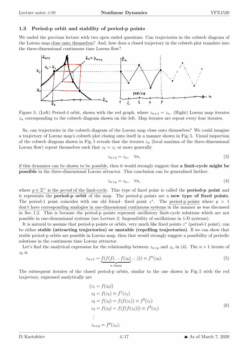
Lecture notes 10 Nonlinear Dynamics YFX1520
13 Period-p orbit and stability of period-p points
We ended the previous lecture with two open ended questions Can trajectories in the cobweb diagram ofthe Lorenz map close onto themselves And how does a closed trajectory in the cobweb plot translate intothe three-dimensional continuous time Lorenz flow
Figure 5 (Left) Period-4 orbit shown with the red graph where zn+4 = zn (Right) Lorenz map iterateszn corresponding to the cobweb diagram shown on the left Map iterates are repeat every four iterates
So can trajectories in the cobweb diagram of the Lorenz map close onto themselves We could imaginea trajectory of Lorenz maprsquos cobweb plot closing onto itself in a manner shown in Fig 5 Visual inspectionof the cobweb diagram shown in Fig 5 reveals that the iterates zn (local maxima of the three-dimensionalLorenz flow) repeat themselves such that z5 = z1 or more generally
zn+4 = zn foralln (3)
if this dynamics can be shown to be possible then it would strongly suggest that a limit-cycle might bepossible in the three-dimensional Lorenz attractor This conclusion can be generalised further
zn+p = zn foralln (4)
where p isin Z+ is the period of the limit-cycle This type of fixed point is called the period-p point andit represents the period-p orbit of the map The period-p points are a new type of fixed pointsThe period-1 point coincides with our old friendmdashfixed point zlowast The period-p points where p gt 1donrsquot have corresponding analogies in one-dimensional continuous systems in the manner as was discussedin Sec 12 This is because the period-p points represent oscillatory limit-cycle solutions which are notpossible in one-dimensional systems (see Lecture 2 Impossibility of oscillations in 1-D systems)
It is natural to assume that period-p points or orbits very much like fixed points zlowast (period-1 point) canbe either stable (attracting trajectories) or unstable (repelling trajectories) If we can show thatstable period-p orbits are possible in Lorenz map then that would strongly suggest a possibility of periodicsolutions in the continuous time Lorenz attractor
Letrsquos find the analytical expression for the relationship between zn+p and zn in (4) The n+ 1 iterate ofz0 is
zn+1 = f(f(f( f(z0)983167 983166983165 983168n times
))) equiv fn(z0) (5)
The subsequent iterates of the closed period-p orbits similar to the one shown in Fig 5 with the redtrajectory expressed analytically are
(z1 = f(z0))
z2 = f(z1) equiv f1(z1)
z3 = f(z2) = f(f(z1)) equiv f2(z1)
z4 = f(z3) = f(f(f(z1))) equiv f3(z1)
zn+p = fp(zn)
(6)
D Kartofelev 417 1003211 As of March 7 2020
Lecture notes 10 Nonlinear Dynamics YFX1520
where z is the period-p point in the period-p orbit and fp is the pth iterate mapDefinition z is a period-p point if equation
fp(z) = z (7)
where p is minimal is satisfiedThe stability of the period-p point is determined via linearisation For simplicity we consider stability of
period-2 pointf2(z) equiv f(f(z)) = z (8)
Note that z is the period-2 point for map f but the fixed point (period-1) for map f2 In the previous lec-ture we showed that the stability of fixed point zlowast depends on the slope of the map at that point Smallperturbations |η| ≪ 1 evolve according to
ηn+1 asymp |f prime(zlowast)|ηn (9)
We find
|(f2(z))prime| = d
dz|f(f(z))| =
983093
983097983097983097983097983095
chain rule+
orbit pointszn+2 = znwe select z1
983094
983098983098983098983098983096= |f prime(f(z1)983167 983166983165 983168
z2
) middot f prime(z1)| = |f prime(z2)| middot |f prime(z1)| gt 1 (10)
because for the Lorenz map |f prime(z)| gt 1 forallz in the map basin The period-2 point is thus unstable Theevolution of perturbations defined by (9) generalised to all period-p points in any closed period-p orbit arethe following
ηn+p asymp
983055983055983055983055983055
pminus1983132
k=0
f prime(zn+k)
983055983055983055983055983055 ηn (11)
here again by the Lorenz map property983055983055983055983055983055
pminus1983132
k=0
f prime(zn+k)
983055983055983055983055983055 gt 1 (12)
Thus all period-p points are unstable The above analysis of the Lorenz map has strongly demonstrated(not proven) that periodic solutions of Lorenz system are not possible and that the flow is indeed long-term aperiodic for t rarr infin
2 1-D maps a proper introduction
This section deals with a new class of dynamical systems (introduced in Lecture 9) in which time is dis-crete rather than continuous These systems are known variously as difference equations recursionrelations iterated maps or simply maps The Lorenz map is such a system When we say ldquomaprdquo dowe mean the function f or the difference equation
xn+1 = f(xn) (13)
Following common usage wersquoll call both of them maps If yoursquore disturbed by this you must be a puremathematician or should consider becoming one Fixed point xlowast of one-dimensional map (13) satisfiesEq (2) and period-p point x satisfies Eq (7) for minimal p
Maps arise in various ways1 As tools for analysing differential equations We have already encountered maps in this role
For instance Lorenz map provided strong evidence that Lorenz attractor is truly strange and is notjust a long-period limit-cycle In future lectures Poincareacute maps will allowed us to prove the existenceof a periodic solutions and to analyse the stability of periodic solutions in general Maps will proveto be superb tools for studying and analysing chaotic systems
D Kartofelev 517 1003211 As of March 7 2020
Lecture notes 10 Nonlinear Dynamics YFX1520
2 As models of natural phenomena In some scientific contexts it is natural to regard time asdiscrete This is the case in digital electronics in parts of economics and finance theory in impulsivelydriven mechanical systems and in the study of certain animal populations where successive generationsdo not overlap
3 As simple examples of chaos Maps are interesting to study in their own right as mathematicallaboratories for chaos Indeed maps are capable of much wilder behaviour than differential equationsbecause the points xn hop along their orbitstrajectoriesiterates rather than flow continuously Con-tinuity is very much a restriction on possible dynamics (see Lecture 6 Poincareacute-Bendixson theorem)
3 Logistic map
xn+1 = xn
Figure 6 Logistic map and the diagonal
In a fascinating and influential review article (linked below) Robert May (1976) emphasised that evensimple nonlinear maps could have very complicated dynamics May illustrated his point with the Logisticmap given by
xn+1 = rxn(1minus xn) (14)
a discrete-time analog of the Logistic equation for population growth where xn is the dimensionless mea-sure of the population in the nth generation and r is the intrinsic growth rate As shown in Fig 6 the graphof map (14) is a parabola with a maximum value of r4 at x = 12 We restrict the control parameter r tothe range (minus2 or) 0 le r le 4 so that Eq (14) maps the interval 0 le x le 1 into itself
Slide 3Logistic map
Logistic map1 has the form
xn+1 = rxn(1 xn) x0 2 [0 1] r 2 [0 4] n 2 Z+ (1)
where r is the control parameter
Read Robert M May ldquoSimple mathematical models with verycomplicated dynamicsrdquo Nature 261 pp 459ndash467 1976doi101038261459a0
1See Mathematica nb file (cobweb diagram and orbit diagram) uploaded tothe course webpage
DKartofelev YFX1520 3 18
Reading suggestion
Link File name CitationPaper1 paper2pdf Robert M May ldquoSimple mathematical models with very complicated dynam-
icsrdquo Nature 261 pp 459ndash467 (1976)doi101038261459a0
D Kartofelev 617 1003211 As of March 7 2020
Lecture notes 10 Nonlinear Dynamics YFX1520
31 Lyapunov exponent
The calculation of Lyapunov exponents of differential equations is not a trivial task In the case of maps itis much easier We remind that the positive Lyapunov exponent λ is a sign of chaos
Slides 4ndash6
Lyapunov exponent of Logistic map
Chaos is characterised by sensitive dependence on initialconditions If we take two close-by initial conditions say x0 andy0 = x0 + with 1 and iterate them under the map then thedicrarrerence between the two time series n = yn xn should growexponentially
|n| |0en| (2)
where is the Lyapunov exponent For maps this definition leads toa very simple way of measuring Lyapunov exponents Solving (2) for gives
=1
nln
n0
(3)
By definition n = fn(x0 + 0) fn(x0) Thus
=1
nln
fn(x0 + 0) fn(x0)
0
(4)
DKartofelev YFX1520 4 18
Lyapunov exponent of Logistic map
For small values of 0 the quantity inside the absolute value signs isjust the derivative of fn with respect to x evaluated at x = x0
=1
nln
dfn
dx
x=x0
(5)
Since fn(x) = f(f(f( f(x))) ) by the chain ruledfn
dx
x=x0
=f 0(fn1(x0)) middot f 0(fn2(x0)) middot middot f 0(x0)
= |f 0(xn1) middot f 0(xn2) middot middot f 0(x0)| =
n1Y
i=0
f 0(xi)
(6)
Our expression for the Lyapunov exponent becomes
=1
nln
n1Y
i=0
f 0(xi)
=1
n
n1X
i=0
ln |f 0(xi)| (7)
DKartofelev YFX1520 5 18
Lyapunov exponent of Logistic map
=1
nln
n1Y
i=0
f 0(xi)
=1
n
n1X
i=0
ln |f 0(xi)|
Lyapunov exponent is the large iterate n limit of this expression andso we have
= limn1
1
n
n1X
i=0
ln |f 0(xi)| (8)
This formula can be used to study Lyapunov exponent2 as a functionof control parameter r
(r) = limn1
1
n
n1X
i=0
ln |f 0(xi r)| (9)
2See Mathematica nb file uploaded to course webpageDKartofelev YFX1520 6 18
The obtained algorithm is used in the following numerical file to calculate the Lyapunov exponent of theLogistic map as a function of the growth rate r
Numerics cdf1 nb1Cobweb diagram and iterates of the (generalised) Lorenz map Lyapunov exponent λ(r) of the Logisticmap
-2 -1 0 1 2 3 4
-3
-2
-1
0
r
Figure 7 Lyapunov exponent of the Logistic map as a function of the growth rate r Calculation uses5000 iterations for every r value plotted
D Kartofelev 717 1003211 As of March 7 2020
Lecture notes 10 Nonlinear Dynamics YFX1520
32 Bifurcation analysis and period doubling bifurcation
Next letrsquos consider only the stable fixed point and stable period-p points as we incrementally increase thevalue of control parameter r ge 0 We do that in order to simplify our analysis and to save some lecturetime The stable fixed point (period-1 point) of Logistic map given by (14) and satisfying condition (2) is
f(xlowast) = xlowast rArr rxlowast(1minus xlowast) = xlowast | divide xlowast (15)
r(1minus xlowast) = 1 (16)
r minus rxlowast = 1 | divide r (17)
1minus xlowast =1
r (18)
xlowast = 1minus 1
r (19)
Additionally there are the trivial solutions xlowast = 0 and xlowast = 1 (for initial condition x0 = xlowast = 1 and forn gt 1 xn rarr xlowast = 0) Fixed point (19) is stable for |f prime(xlowast)| lt 1 Using map definition (14) we write
|f prime(xlowast)| =983055983055[rx(1minus x)]prime
983055983055x=xlowast = |r minus 2rxlowast| lt 1 (20)
Using condition (20) and for the trivial fixed point xlowast = 0 we get
|r minus 0| lt 1 (21)
|r| lt 1 (22)
The other trivial fixed point xlowast = 1 gives the same result
|r minus 2r| lt 1 (23)
|minus r| lt 1 (24)
Thus the fixed points xlowast = 0 and xlowast = 1 are stable for |plusmnr| lt 1 For the non-trivial fixed point xlowast = 1minus1rand for condition (20) we find 983055983055983055983055r minus 2r
9830611minus 1
r
983062983055983055983055983055 lt 1 (25)
|r minus 2r + 2| lt 1 (26)
|2minus r| lt 1 (27)
1 lt |r| lt 3 (28)
The fixed points xlowast = 1minus 1r exist and is stable for 1 lt |r| lt 3It seems that the found intervals (22) (24) and (28) excluded r = 1 (obviously it does not satisfy
|f prime(xlowast)| lt 1) Letrsquos find the value of the map slope |f prime(xlowast)| for r = 1 using (20) in the case of the trivialsolutions xlowast = 0
|f prime(xlowast)| = |1minus 0| = 1 (29)
xlowast = 1|f prime(xlowast)| = |1minus 2| = 1 (30)
and in the non-trivial case for xlowast = 1minus 1r = 1minus 1 = 0 Which should obviously generate the same result
|f prime(xlowast)| =9830559830559830559830551minus 2
9830611minus 1
1
983062983055983055983055983055 = |1minus 0| = 1 (31)
Below it will also be beneficial to know what happens for r = 3 the r value just after the interval (28)We consider the non-trivial fixed point xlowast = 1minus 1r and find the slope
|f prime(xlowast)| =9830559830559830559830553minus 2 middot 3
9830611minus 1
3
983062983055983055983055983055 = |3minus 4| = |minus 1| = 1 (32)
Usually slope |f prime(xlowast)| = 1 corresponds to the (period doubling or flip) bifurcation point Values r = 1and r = 3 are the bifurcation points Figure 8 shows the map positions of the fixed points and map slopes|f prime(xlowast)| evaluated at the non-trivial fixed point xlowast = 1minus 1r for r = 1 and r = 3
D Kartofelev 817 1003211 As of March 7 2020
Lecture notes 10 Nonlinear Dynamics YFX1520
Figure 8 (Left) Map slope at the fixed points xlowast = 1 minus 1r (same as the trivial case xlowast = 0) for r = 1(Right) Map slope at the fixed points xlowast = 1minus 1r for r = 3
The following interactive numerical file show the dynamics of Logistic map for 0 le |r| lt 1 and 1 lt |r| lt 3
Numerics cdf2 nb2Cobweb diagram of the Logistic map Orbit diagram of the Logistic map Period doubling and orbitdiagram
00 02 04 06 08 1000
02
04
06
08
10
xn
xn+1
0 5 10 15 2000
02
04
06
08
10
n
xn
00 02 04 06 08 1000
02
04
06
08
10
xn
xn+1
0 5 10 15 2000
02
04
06
08
10
n
xn
Figure 9 (Top-left) Cobweb diagram of the Logistic map shown for r = 098 lt 1 The fixed pointxlowast = 0 (Top-right) Map iterates corresponding to the cobweb diagram shown on the left (Bottom-left)Cobweb diagram of the Logistic map shown for interval 1 lt |r| lt 3 with r = 282 The fixed pointxlowast = 1minus 1r (Bottom-right) Map iterates corresponding to the cobweb diagram shown on the left
What happens for r ge 3 What happens after the period doubling or flip bifurcation at r = 3 Thename ldquofliprdquo refers to the fact that the map trajectories start to flip between two values mdash period-2 pointsin period-2 orbit Letrsquos check the dynamics using a computer
Numerics cdf2 nb2Cobweb diagram of the Logistic map Orbit diagram of the Logistic map Period doubling and orbitdiagramAfter the initial transient behaviour has decayed the dynamics of the map settles to a stableperiod-2 orbit It can be showed that period-2 orbits exist for 3 le r lt 1 +
radic6
D Kartofelev 917 1003211 As of March 7 2020
Lecture notes 10 Nonlinear Dynamics YFX1520
00 02 04 06 08 1000
02
04
06
08
10
xn
xn+1
0 5 10 15 20 25 3000
02
04
06
08
10
n
xn
Figure 10 (Left) Cobweb diagram of the Logistic map shown for r = 319 ge 3 featuring the stableperiod-2 point (Right) Map iterates corresponding to the cobweb diagram shown on the left
Letrsquos try to think about this outcome some more
Slides 7ndash9
Logistic map period-2 window
Period-2 window for 3 r lt 1 +p6
Figure Logistic map where r = 318 and x0 = 035 Fixed points (fps)in the case where r lt 3 are shown with the grey bullets Period-2 pointsof f(x) map for r 3 are shown with the blue bullets The fixed points off2(x) map for r 3 are shown with the red bullets
DKartofelev YFX1520 7 18
Logistic map period-2 window
Period-2 window for 3 r lt 1 +p6
(f(p) = rp(1 p) = q
f(q) = rq(1 q) = p(10)
where period-2 point values p and q are the fps of f(x) map
On the other hand it also holds(f(p) = f(f(q)) f 2(q) = r[rq(1 q)][1 (rq(1 q))] = q
f(q) = f(f(p)) f 2(p) = r[rp(1 p)][1 (rp(1 p))] = p)
(11)) f 2(x) = r[rx(1 x)][1 (rx(1 x))] = x (12)
where period-2 point values p and q are the fps of f 2(x) map
DKartofelev YFX1520 8 18
If you want to study the dynamics of the attractors of second iterate map f2 analytically consider oneof the equations in (11 slide numbering) The fourth order polynomial defined by Eq (7)
r[rx(1minus x)][1minus (rx(1minus x))] = x (33)
minus r3x4 + 2r3x3 minus r2(1 + r)x2 + r2x = x (34)
Intersections between the graph of second iterate map f2 and the diagonal correspond to the solutionsof f2(x) = x (34)
Stability of fps of f 2map in period-2 orbit
We need to know the slopes of period-2 points(f(p) = rp(1 p) = q
f(q) = rq(1 q) = p
According to the chain rule it holds that
(f 2(x))0 (f(f(x))0 = f 0(f(x)) middot f 0(x) (13)
In our case
(f 2(p))0 = f 0(f(p)) middot f 0(p) = f 0(q) middot f 0(p)
(f 2(q))0 = f 0(f(q)) middot f 0(q) = f 0(p) middot f 0(q)
)) (f 2(p))0 = (f 2(q))0
(14)Above follows from the commutative property of multiplication
DKartofelev YFX1520 9 18
D Kartofelev 1017 1003211 As of March 7 2020
Lecture notes 10 Nonlinear Dynamics YFX1520
The slopes of map f2 at its fixed points p and q are equal and they are the products of map f slopesat its respective period-2 points
What happens for r ge 1 +radic6 Once again we use a computer
Numerics cdf2 nb2Cobweb diagram of the Logistic map Orbit diagram of the Logistic map Period doubling and orbitdiagram
A period-4 orbit has emerged It can be shown that period-4 orbits exist for 1 +radic6 le r lt 354409
00 02 04 06 08 1000
02
04
06
08
10
xn
xn+1
0 5 10 15 20 25 3000
02
04
06
08
10
n
xn
Figure 11 (Left) Cobweb diagram of the Logistic map shown for r = 3535 ge 1 +radic6 featuring the
stable period-4 point The blue graph shows fourth iterate map f4 (Right) Map iterates correspondingto the cobweb diagram of map f shown on the left
Figure 12 counts the period-4 pointsiterates in the period-4 orbit of the Logistic map Compare Fig 12 toFig 5
Figure 12 Period-4 orbit in the Logistic map
What have we seen so far As we have incrementally increased the value of control parameter r theperiods of the fixed points have increased as well mdash from period-1 to period-2 and finally to period-4The period is clearly doubling This type of bifurcation is called the period doubling bifurca-tion Further period-doublings to orbits of period-8 -16 -32 etc occur as r increases Specifically letrn denote the value of r where a stable 2n-orbit first appears Then computer experiments reveal that
D Kartofelev 1117 1003211 As of March 7 2020
Lecture notes 10 Nonlinear Dynamics YFX1520
Slide 10
Logistic map period doubling
Even number periods
rn ndash bifurcation point onset of stable period-2n orbit
r1 = 30 period-2r2 = 1 +
p6 344949 period-4
r3 354409 period-8r4 356441 period-16r5 356875 period-32r6 356969 period-64
r1 3569946 period-21
r1 ndash onset of chaos (the accumulation point)
= limn1
rn1 rn2
rn rn1 4669201609 (15)
DKartofelev YFX1520 10 18
Note that the successive bifurcations come faster and faster Ultimately the rn converge toa limiting value rinfin The convergence is (essentially) geometric (itrsquos geometric near rinfin) in the limitof large n the distance between successive transitions shrinks by a constant factor of δ This ratio iscalled the Feigenbaum constant After the accumulation point r gt rinfin the dynamics becomeschaotic as wersquoll see below
33 Orbit diagram
The orbit diagram is also called the fig tree diagram (Feigenbaum in German means ldquofig treerdquo) or (in-correctly) the Feigenbaum diagram You might guess that the system would become more and morechaotic for r gt rinfin as r increases but in fact the dynamics are more subtle than that To see the long-termbehaviour for all values of r at once we plot the orbit diagram a special kind of bifurcation diagramOrbit diagram plots the systemrsquos attractor (stable fixed points and stable period-p points) as a function ofcontrol parameter r
To generate the orbit diagram for yourself yoursquoll need to write a computer program with two loops Firstchoose a value of r Then generate an orbit starting from some random initial condition x0 Iterate for 300cycles or so to allow the system to settle down to its eventual stable behaviour Once the transients havedecayed plot many points say x301 x900 above that r Then move to an adjacent value of r and repeateventually sweeping across the whole diagram
The following interactive numerical file shows the orbit diagram for the Logistic map
Numerics cdf2 nb2Cobweb diagram of the Logistic map Orbit diagram of the Logistic map Period doubling and orbitdiagram
The connection between the cobweb diagram orbit diagram and the Lyapunov exponent is shown in theinteractive numerical file linked below
Numerics cdf3 nb3Logistic map cobweb diagram orbit diagram and map iterates Lyapunov exponent
D Kartofelev 1217 1003211 As of March 7 2020
Lecture notes 10 Nonlinear Dynamics YFX1520
Slides 11 12
Orbit diagram and period doubling
DKartofelev YFX1520 11 18
Zooming into the Logistic map self-similarity
No embedded video files in this pdf
DKartofelev YFX1520 12 18
The period doubling is driven by the subsequent flip bifurcations or supercritical pitchforkbifurcations (if we use the nomenclature introduced in Lecture 2) The unstable fixed point andperiod-p points are omitted from the orbit diagram
Feigenbaum diagram shows both stable and unstable fixed points and period-p points or simplydiagram branches (not shown here)
The orbit diagram of the Logistic map features self-similarity In mathematics a self-similarobject is (exactly or) approximately similar to a part of itself ie the whole has the same shape orquality as one or more of its sub-parts
34 Tangent bifurcation and odd number period-p points
Can an odd number period appear in the Logistic map mdash eg period-3 point One of the most intriguingfeatures of the orbit diagram is the occurrence of periodic windows for r gt rinfin The period-3 windowthat occurs for 1 +
radic8 le r le 38415 is the most conspicuous Suddenly against a backdrop of chaos a
stable period-3 orbit appears out of the blueLetrsquos see if we can find the period-3 window of Logistic map using a computer
Numerics cdf2 nb2Cobweb diagram of the Logistic map Orbit diagram of the Logistic map Period doubling and orbitdiagram
The tangent bifurcation is a new type of bifurcation for us that occurs at r = 1 +radic8
00 02 04 06 08 1000
02
04
06
08
10
xn
xn+1
0 5 10 15 20 25 3000
02
04
06
08
10
n
xn
Figure 13 (Left) Period-3 orbit of map f can be found in the period-3 window Here showing thetrajectory for r = 383 (Right) Map iterates corresponding to the cobweb diagram of map f shownon the left
The mechanism responsible for the occurrence of the odd number periods-p points is shown in Fig 14The intersections between the graph of f3 shown in red and the diagonal correspond to solutions of
D Kartofelev 1317 1003211 As of March 7 2020
Lecture notes 10 Nonlinear Dynamics YFX1520
Figure 14 Period-3 orbit can be found in period-3 window of the orbit diagram
f3(x) = x There are eight solutions for r ge 1+radic8 six of interest to us are marked with the blue dots and
two imposters that are not genuine period-3 they are actually fixed points or period-1 points for whichf(xlowast) = xlowast The blue filled dots in Fig 14 correspond to a stable period-3 cycle note that the slope off3(x) is shallow at these points consistent with the stability of the cycle In contrast the slope exceeds 1at the cycle marked by the empty blue dots this period-3 orbit is therefore unstable
Now suppose we decrease r toward the chaotic regime r lt 1+radic8 Then the red graph in Fig 14 changes
shape mdash the hill moves down and the valleys rise up The curve therefore moves towards the diagonalFigure 14 shows that when r = 1 +
radic8 the six blue intersections have merged to form three black filled
period-3 points by becoming tangent to the diagonal At this critical value of r the stable and unstableperiod-3 cycles coalesce and annihilate in a tangent bifurcation This transition defines the beginning ofthe periodic period-3 window
All odd number periods will also undergo the period doubling This means that all number periods [1infin)are eventually represented in the orbit diagram
Figure 14 also explains the self-similarity present in the orbit diagram as shown on Slide 12 for differentscales of magnification The peaks and valley of map f3 are smaller distorted copies of the original mapf Thus the local dynamics of the cobweb trajectories for map f3 must be similar to the dynamics of theoriginal map f
Slide 13
Intermittency3and period-3 window
Transient chaos and intermittency in dynamical systemsTangent bifurcation occurs at r = 1 +
p8 38284 (period-3 orbit)
50 100 150n
02
04
06
08
10xn
Iterates of Logistic map shown for r = 38282 and x0 = 015
3See Mathematica nb file uploaded to course webpageDKartofelev YFX1520 13 18
The dynamics closely related to the tangent bifurcation is intermittency Logistic map exhibitsintermittent chaos for r values just before the period-3 window
D Kartofelev 1417 1003211 As of March 7 2020
Lecture notes 10 Nonlinear Dynamics YFX1520
Numerics cdf4 nb4Period-3 window and intermittency in the Logistic map (iterates xn)
4 Sine map and universality of period doubling
It can be shown that in all unimodal maps same dynamics of period doubling occurs For example weconsider the sine map
Slide 14
Universality of period doubling in unimodal maps
1-D sine map4 The sine map has the form
xn+1 = r sin(xn) x0 2 [0 1] r 2 [0 1] n 2 Z+ (16)
where r is the control parameter
Read Mitchell J Feigenbaum ldquoQuantitative universality for a classof nonlinear transformationsrdquo Journal of Statistical Physics 19(1)pp 25ndash52 1978 doi101007BF01020332
Read Mitchell J Feigenbaum ldquoUniversal behavior in nonlinearsystemsrdquo Physica D Nonlinear Phenomena 7(1ndash3) pp 16ndash391983 doi1010160167-2789(83)90112-4
4See Mathematica nb file (cobweb diagram and orbit diagram) uploaded tothe course webpage
DKartofelev YFX1520 14 18
The graph of the sine map has the same basic shape as the graph of the Logistic map Both curvesare smooth concave down and have a single maximum Such maps are called unimodal
Sine is also a transcendental function opposed to an algebraic function as is the polynomial thatdescribes the Logistic map A transcendental function is an analytic function that does not satisfy apolynomial equation In other words a transcendental function ldquotranscendsrdquo algebra in that it cannotbe expressed in terms of a finite sequence of the algebraic operations of addition multiplication androot extraction
The transcendental nature of the sine map must makes the underlying higher-dimensional physicsrepresented by the sine map fundamentally different from eg the three-dimensional Lorenz flowsampled by Lorenz map
Letrsquos study the dynamics of the sine map using a computer
Numerics cdf5 nb5The sine map iterates cobweb and orbit diagrams (xn isin [0 1])
Numerics cdf6 nb6The sine map iterates cobweb and orbit diagrams (xn isin [minus1 1])
The dynamics is surprisingly similar to the dynamics of the Logistic map Mitchell J Feigenbaumwas first to discover the quantitative laws that are independent of unimodal map functions f Bythat we mean that the algebraic form of f(x) is irrelevant only its overall shape matters
D Kartofelev 1517 1003211 As of March 7 2020
Lecture notes 10 Nonlinear Dynamics YFX1520
Slide 151-D unimodal maps and Feigenbaum constants
= limn1
n1
n= lim
n1
rn1 rn2
rn rn1 4669201609 (17)
crarr = limn1
dn1
dn 2502907875 (18)
DKartofelev YFX1520 15 18
Here xm = max f(x) is the maximum of the map graph The Feigenbaum constants are valid up tothe onset of chaos at rinfin and inside each periodic window for r gt rinfin
In addition to scaling law in control parameter r direction shown earlier Feigenbaum also foundscaling law for the vertical x-direction of the orbit diagram The Feigenbaum constants are uni-versal the same convergence rate appears no matter what unimodal map is iterated They are newmathematical constants as basic to period doubling as π is to circles
Reading suggestion
Link File name CitationPaper2 paper3pdf Mitchell J Feigenbaum ldquoQuantitative universality for a class of nonlinear trans-
formationsrdquo Journal of Statistical Physics 19(1) pp 25ndash52 (1978)doi101007BF01020332
Paper3 paper4pdf Mitchell J Feigenbaum ldquoUniversal behavior in nonlinear systemsrdquo Physica DNonlinear Phenomena 7(1ndash3) pp 16ndash39 (1983)doi1010160167-2789(83)90112-4
5 Universal route to chaos
We showed that the qualitative dynamics of the Logistic and sine maps are identical They both undergoperiod doubling routes to chaos followed by periodic windows interwoven with chaotic bandsEven more remarkably the periodic windows occur in the same order and with the same relative sizes Forinstance the period-3 window is the largest in both cases and the next largest windows preceding it areperiod-5 and period-6 But there are quantitative differences For instance the period doubling bifurcationsoccur later (for greater parameter r value) in the Logistic map and the periodic windows are thinner
Turns out that the onset of chaos via period doubling is predominant in nature and in artificial chaoticsystems Feigenbaum constants have real predictive power in various scientific applications The perioddoubling bifurcation is the ldquorouterdquo taken by nonlinear systems to reach chaotic solution Interm of the bifurcations introduced in Lecture 2 the period doubling bifurcation can also be seen as a seriesof subsequentsucceeding supercritical pitchfork bifurcations see Slide 11
Revision questions
1 What is cobweb diagram2 What is recurrence map or recurrence relation3 What is 1-D map4 How to find fixed points of 1-D maps5 What is Lorenz map
D Kartofelev 1617 1003211 As of March 7 2020
Lecture notes 10 Nonlinear Dynamics YFX1520
6 What is Logistic map7 What is sine map8 What is period doubling9 What is period doubling bifurcation
10 What is tangent bifurcation11 Do odd number periods (period-p orbits) exist in chaotic systems12 Do even number periods (period-p orbits) exist in chaotic systems13 Can maps produce transient chaos14 Can maps produce intermittency15 Can maps produce intermittent chaos16 What is orbit diagram (or Feigenbaum diagram)17 What are Feigenbaum constants
D Kartofelev 1717 1003211 As of March 7 2020
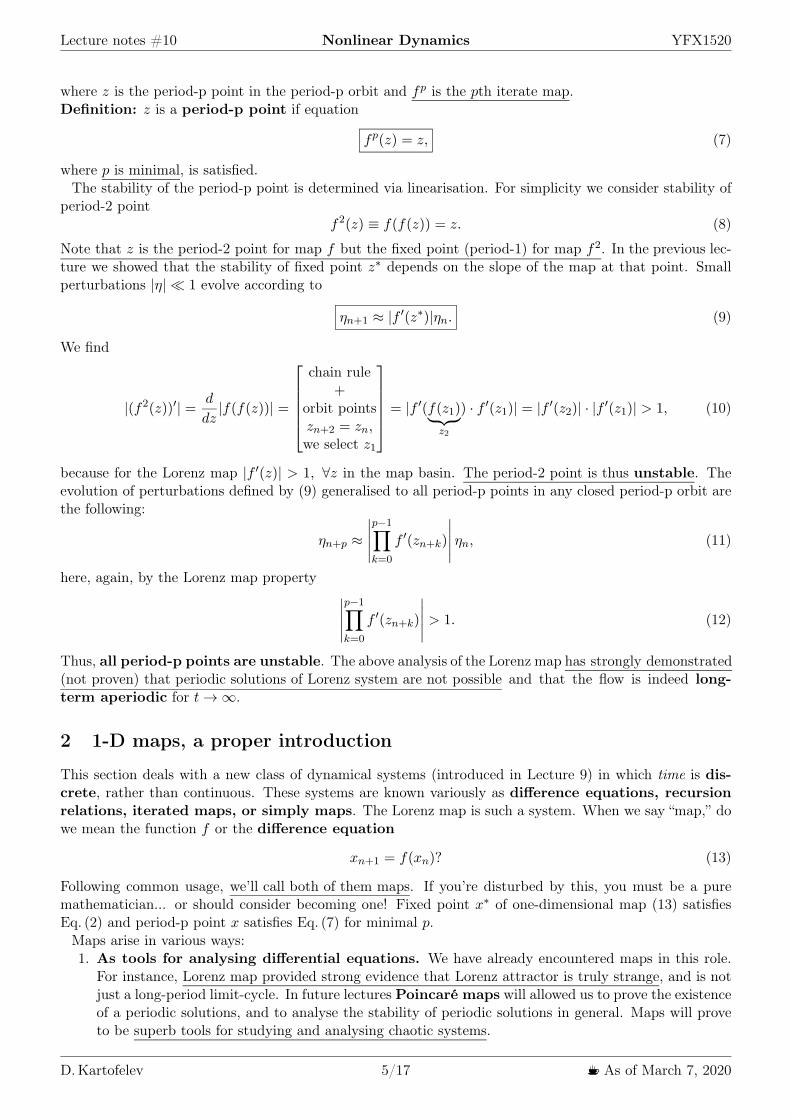
Lecture notes 10 Nonlinear Dynamics YFX1520
where z is the period-p point in the period-p orbit and fp is the pth iterate mapDefinition z is a period-p point if equation
fp(z) = z (7)
where p is minimal is satisfiedThe stability of the period-p point is determined via linearisation For simplicity we consider stability of
period-2 pointf2(z) equiv f(f(z)) = z (8)
Note that z is the period-2 point for map f but the fixed point (period-1) for map f2 In the previous lec-ture we showed that the stability of fixed point zlowast depends on the slope of the map at that point Smallperturbations |η| ≪ 1 evolve according to
ηn+1 asymp |f prime(zlowast)|ηn (9)
We find
|(f2(z))prime| = d
dz|f(f(z))| =
983093
983097983097983097983097983095
chain rule+
orbit pointszn+2 = znwe select z1
983094
983098983098983098983098983096= |f prime(f(z1)983167 983166983165 983168
z2
) middot f prime(z1)| = |f prime(z2)| middot |f prime(z1)| gt 1 (10)
because for the Lorenz map |f prime(z)| gt 1 forallz in the map basin The period-2 point is thus unstable Theevolution of perturbations defined by (9) generalised to all period-p points in any closed period-p orbit arethe following
ηn+p asymp
983055983055983055983055983055
pminus1983132
k=0
f prime(zn+k)
983055983055983055983055983055 ηn (11)
here again by the Lorenz map property983055983055983055983055983055
pminus1983132
k=0
f prime(zn+k)
983055983055983055983055983055 gt 1 (12)
Thus all period-p points are unstable The above analysis of the Lorenz map has strongly demonstrated(not proven) that periodic solutions of Lorenz system are not possible and that the flow is indeed long-term aperiodic for t rarr infin
2 1-D maps a proper introduction
This section deals with a new class of dynamical systems (introduced in Lecture 9) in which time is dis-crete rather than continuous These systems are known variously as difference equations recursionrelations iterated maps or simply maps The Lorenz map is such a system When we say ldquomaprdquo dowe mean the function f or the difference equation
xn+1 = f(xn) (13)
Following common usage wersquoll call both of them maps If yoursquore disturbed by this you must be a puremathematician or should consider becoming one Fixed point xlowast of one-dimensional map (13) satisfiesEq (2) and period-p point x satisfies Eq (7) for minimal p
Maps arise in various ways1 As tools for analysing differential equations We have already encountered maps in this role
For instance Lorenz map provided strong evidence that Lorenz attractor is truly strange and is notjust a long-period limit-cycle In future lectures Poincareacute maps will allowed us to prove the existenceof a periodic solutions and to analyse the stability of periodic solutions in general Maps will proveto be superb tools for studying and analysing chaotic systems
D Kartofelev 517 1003211 As of March 7 2020
Lecture notes 10 Nonlinear Dynamics YFX1520
2 As models of natural phenomena In some scientific contexts it is natural to regard time asdiscrete This is the case in digital electronics in parts of economics and finance theory in impulsivelydriven mechanical systems and in the study of certain animal populations where successive generationsdo not overlap
3 As simple examples of chaos Maps are interesting to study in their own right as mathematicallaboratories for chaos Indeed maps are capable of much wilder behaviour than differential equationsbecause the points xn hop along their orbitstrajectoriesiterates rather than flow continuously Con-tinuity is very much a restriction on possible dynamics (see Lecture 6 Poincareacute-Bendixson theorem)
3 Logistic map
xn+1 = xn
Figure 6 Logistic map and the diagonal
In a fascinating and influential review article (linked below) Robert May (1976) emphasised that evensimple nonlinear maps could have very complicated dynamics May illustrated his point with the Logisticmap given by
xn+1 = rxn(1minus xn) (14)
a discrete-time analog of the Logistic equation for population growth where xn is the dimensionless mea-sure of the population in the nth generation and r is the intrinsic growth rate As shown in Fig 6 the graphof map (14) is a parabola with a maximum value of r4 at x = 12 We restrict the control parameter r tothe range (minus2 or) 0 le r le 4 so that Eq (14) maps the interval 0 le x le 1 into itself
Slide 3Logistic map
Logistic map1 has the form
xn+1 = rxn(1 xn) x0 2 [0 1] r 2 [0 4] n 2 Z+ (1)
where r is the control parameter
Read Robert M May ldquoSimple mathematical models with verycomplicated dynamicsrdquo Nature 261 pp 459ndash467 1976doi101038261459a0
1See Mathematica nb file (cobweb diagram and orbit diagram) uploaded tothe course webpage
DKartofelev YFX1520 3 18
Reading suggestion
Link File name CitationPaper1 paper2pdf Robert M May ldquoSimple mathematical models with very complicated dynam-
icsrdquo Nature 261 pp 459ndash467 (1976)doi101038261459a0
D Kartofelev 617 1003211 As of March 7 2020
Lecture notes 10 Nonlinear Dynamics YFX1520
31 Lyapunov exponent
The calculation of Lyapunov exponents of differential equations is not a trivial task In the case of maps itis much easier We remind that the positive Lyapunov exponent λ is a sign of chaos
Slides 4ndash6
Lyapunov exponent of Logistic map
Chaos is characterised by sensitive dependence on initialconditions If we take two close-by initial conditions say x0 andy0 = x0 + with 1 and iterate them under the map then thedicrarrerence between the two time series n = yn xn should growexponentially
|n| |0en| (2)
where is the Lyapunov exponent For maps this definition leads toa very simple way of measuring Lyapunov exponents Solving (2) for gives
=1
nln
n0
(3)
By definition n = fn(x0 + 0) fn(x0) Thus
=1
nln
fn(x0 + 0) fn(x0)
0
(4)
DKartofelev YFX1520 4 18
Lyapunov exponent of Logistic map
For small values of 0 the quantity inside the absolute value signs isjust the derivative of fn with respect to x evaluated at x = x0
=1
nln
dfn
dx
x=x0
(5)
Since fn(x) = f(f(f( f(x))) ) by the chain ruledfn
dx
x=x0
=f 0(fn1(x0)) middot f 0(fn2(x0)) middot middot f 0(x0)
= |f 0(xn1) middot f 0(xn2) middot middot f 0(x0)| =
n1Y
i=0
f 0(xi)
(6)
Our expression for the Lyapunov exponent becomes
=1
nln
n1Y
i=0
f 0(xi)
=1
n
n1X
i=0
ln |f 0(xi)| (7)
DKartofelev YFX1520 5 18
Lyapunov exponent of Logistic map
=1
nln
n1Y
i=0
f 0(xi)
=1
n
n1X
i=0
ln |f 0(xi)|
Lyapunov exponent is the large iterate n limit of this expression andso we have
= limn1
1
n
n1X
i=0
ln |f 0(xi)| (8)
This formula can be used to study Lyapunov exponent2 as a functionof control parameter r
(r) = limn1
1
n
n1X
i=0
ln |f 0(xi r)| (9)
2See Mathematica nb file uploaded to course webpageDKartofelev YFX1520 6 18
The obtained algorithm is used in the following numerical file to calculate the Lyapunov exponent of theLogistic map as a function of the growth rate r
Numerics cdf1 nb1Cobweb diagram and iterates of the (generalised) Lorenz map Lyapunov exponent λ(r) of the Logisticmap
-2 -1 0 1 2 3 4
-3
-2
-1
0
r
Figure 7 Lyapunov exponent of the Logistic map as a function of the growth rate r Calculation uses5000 iterations for every r value plotted
D Kartofelev 717 1003211 As of March 7 2020
Lecture notes 10 Nonlinear Dynamics YFX1520
32 Bifurcation analysis and period doubling bifurcation
Next letrsquos consider only the stable fixed point and stable period-p points as we incrementally increase thevalue of control parameter r ge 0 We do that in order to simplify our analysis and to save some lecturetime The stable fixed point (period-1 point) of Logistic map given by (14) and satisfying condition (2) is
f(xlowast) = xlowast rArr rxlowast(1minus xlowast) = xlowast | divide xlowast (15)
r(1minus xlowast) = 1 (16)
r minus rxlowast = 1 | divide r (17)
1minus xlowast =1
r (18)
xlowast = 1minus 1
r (19)
Additionally there are the trivial solutions xlowast = 0 and xlowast = 1 (for initial condition x0 = xlowast = 1 and forn gt 1 xn rarr xlowast = 0) Fixed point (19) is stable for |f prime(xlowast)| lt 1 Using map definition (14) we write
|f prime(xlowast)| =983055983055[rx(1minus x)]prime
983055983055x=xlowast = |r minus 2rxlowast| lt 1 (20)
Using condition (20) and for the trivial fixed point xlowast = 0 we get
|r minus 0| lt 1 (21)
|r| lt 1 (22)
The other trivial fixed point xlowast = 1 gives the same result
|r minus 2r| lt 1 (23)
|minus r| lt 1 (24)
Thus the fixed points xlowast = 0 and xlowast = 1 are stable for |plusmnr| lt 1 For the non-trivial fixed point xlowast = 1minus1rand for condition (20) we find 983055983055983055983055r minus 2r
9830611minus 1
r
983062983055983055983055983055 lt 1 (25)
|r minus 2r + 2| lt 1 (26)
|2minus r| lt 1 (27)
1 lt |r| lt 3 (28)
The fixed points xlowast = 1minus 1r exist and is stable for 1 lt |r| lt 3It seems that the found intervals (22) (24) and (28) excluded r = 1 (obviously it does not satisfy
|f prime(xlowast)| lt 1) Letrsquos find the value of the map slope |f prime(xlowast)| for r = 1 using (20) in the case of the trivialsolutions xlowast = 0
|f prime(xlowast)| = |1minus 0| = 1 (29)
xlowast = 1|f prime(xlowast)| = |1minus 2| = 1 (30)
and in the non-trivial case for xlowast = 1minus 1r = 1minus 1 = 0 Which should obviously generate the same result
|f prime(xlowast)| =9830559830559830559830551minus 2
9830611minus 1
1
983062983055983055983055983055 = |1minus 0| = 1 (31)
Below it will also be beneficial to know what happens for r = 3 the r value just after the interval (28)We consider the non-trivial fixed point xlowast = 1minus 1r and find the slope
|f prime(xlowast)| =9830559830559830559830553minus 2 middot 3
9830611minus 1
3
983062983055983055983055983055 = |3minus 4| = |minus 1| = 1 (32)
Usually slope |f prime(xlowast)| = 1 corresponds to the (period doubling or flip) bifurcation point Values r = 1and r = 3 are the bifurcation points Figure 8 shows the map positions of the fixed points and map slopes|f prime(xlowast)| evaluated at the non-trivial fixed point xlowast = 1minus 1r for r = 1 and r = 3
D Kartofelev 817 1003211 As of March 7 2020
Lecture notes 10 Nonlinear Dynamics YFX1520
Figure 8 (Left) Map slope at the fixed points xlowast = 1 minus 1r (same as the trivial case xlowast = 0) for r = 1(Right) Map slope at the fixed points xlowast = 1minus 1r for r = 3
The following interactive numerical file show the dynamics of Logistic map for 0 le |r| lt 1 and 1 lt |r| lt 3
Numerics cdf2 nb2Cobweb diagram of the Logistic map Orbit diagram of the Logistic map Period doubling and orbitdiagram
00 02 04 06 08 1000
02
04
06
08
10
xn
xn+1
0 5 10 15 2000
02
04
06
08
10
n
xn
00 02 04 06 08 1000
02
04
06
08
10
xn
xn+1
0 5 10 15 2000
02
04
06
08
10
n
xn
Figure 9 (Top-left) Cobweb diagram of the Logistic map shown for r = 098 lt 1 The fixed pointxlowast = 0 (Top-right) Map iterates corresponding to the cobweb diagram shown on the left (Bottom-left)Cobweb diagram of the Logistic map shown for interval 1 lt |r| lt 3 with r = 282 The fixed pointxlowast = 1minus 1r (Bottom-right) Map iterates corresponding to the cobweb diagram shown on the left
What happens for r ge 3 What happens after the period doubling or flip bifurcation at r = 3 Thename ldquofliprdquo refers to the fact that the map trajectories start to flip between two values mdash period-2 pointsin period-2 orbit Letrsquos check the dynamics using a computer
Numerics cdf2 nb2Cobweb diagram of the Logistic map Orbit diagram of the Logistic map Period doubling and orbitdiagramAfter the initial transient behaviour has decayed the dynamics of the map settles to a stableperiod-2 orbit It can be showed that period-2 orbits exist for 3 le r lt 1 +
radic6
D Kartofelev 917 1003211 As of March 7 2020
Lecture notes 10 Nonlinear Dynamics YFX1520
00 02 04 06 08 1000
02
04
06
08
10
xn
xn+1
0 5 10 15 20 25 3000
02
04
06
08
10
n
xn
Figure 10 (Left) Cobweb diagram of the Logistic map shown for r = 319 ge 3 featuring the stableperiod-2 point (Right) Map iterates corresponding to the cobweb diagram shown on the left
Letrsquos try to think about this outcome some more
Slides 7ndash9
Logistic map period-2 window
Period-2 window for 3 r lt 1 +p6
Figure Logistic map where r = 318 and x0 = 035 Fixed points (fps)in the case where r lt 3 are shown with the grey bullets Period-2 pointsof f(x) map for r 3 are shown with the blue bullets The fixed points off2(x) map for r 3 are shown with the red bullets
DKartofelev YFX1520 7 18
Logistic map period-2 window
Period-2 window for 3 r lt 1 +p6
(f(p) = rp(1 p) = q
f(q) = rq(1 q) = p(10)
where period-2 point values p and q are the fps of f(x) map
On the other hand it also holds(f(p) = f(f(q)) f 2(q) = r[rq(1 q)][1 (rq(1 q))] = q
f(q) = f(f(p)) f 2(p) = r[rp(1 p)][1 (rp(1 p))] = p)
(11)) f 2(x) = r[rx(1 x)][1 (rx(1 x))] = x (12)
where period-2 point values p and q are the fps of f 2(x) map
DKartofelev YFX1520 8 18
If you want to study the dynamics of the attractors of second iterate map f2 analytically consider oneof the equations in (11 slide numbering) The fourth order polynomial defined by Eq (7)
r[rx(1minus x)][1minus (rx(1minus x))] = x (33)
minus r3x4 + 2r3x3 minus r2(1 + r)x2 + r2x = x (34)
Intersections between the graph of second iterate map f2 and the diagonal correspond to the solutionsof f2(x) = x (34)
Stability of fps of f 2map in period-2 orbit
We need to know the slopes of period-2 points(f(p) = rp(1 p) = q
f(q) = rq(1 q) = p
According to the chain rule it holds that
(f 2(x))0 (f(f(x))0 = f 0(f(x)) middot f 0(x) (13)
In our case
(f 2(p))0 = f 0(f(p)) middot f 0(p) = f 0(q) middot f 0(p)
(f 2(q))0 = f 0(f(q)) middot f 0(q) = f 0(p) middot f 0(q)
)) (f 2(p))0 = (f 2(q))0
(14)Above follows from the commutative property of multiplication
DKartofelev YFX1520 9 18
D Kartofelev 1017 1003211 As of March 7 2020
Lecture notes 10 Nonlinear Dynamics YFX1520
The slopes of map f2 at its fixed points p and q are equal and they are the products of map f slopesat its respective period-2 points
What happens for r ge 1 +radic6 Once again we use a computer
Numerics cdf2 nb2Cobweb diagram of the Logistic map Orbit diagram of the Logistic map Period doubling and orbitdiagram
A period-4 orbit has emerged It can be shown that period-4 orbits exist for 1 +radic6 le r lt 354409
00 02 04 06 08 1000
02
04
06
08
10
xn
xn+1
0 5 10 15 20 25 3000
02
04
06
08
10
n
xn
Figure 11 (Left) Cobweb diagram of the Logistic map shown for r = 3535 ge 1 +radic6 featuring the
stable period-4 point The blue graph shows fourth iterate map f4 (Right) Map iterates correspondingto the cobweb diagram of map f shown on the left
Figure 12 counts the period-4 pointsiterates in the period-4 orbit of the Logistic map Compare Fig 12 toFig 5
Figure 12 Period-4 orbit in the Logistic map
What have we seen so far As we have incrementally increased the value of control parameter r theperiods of the fixed points have increased as well mdash from period-1 to period-2 and finally to period-4The period is clearly doubling This type of bifurcation is called the period doubling bifurca-tion Further period-doublings to orbits of period-8 -16 -32 etc occur as r increases Specifically letrn denote the value of r where a stable 2n-orbit first appears Then computer experiments reveal that
D Kartofelev 1117 1003211 As of March 7 2020
Lecture notes 10 Nonlinear Dynamics YFX1520
Slide 10
Logistic map period doubling
Even number periods
rn ndash bifurcation point onset of stable period-2n orbit
r1 = 30 period-2r2 = 1 +
p6 344949 period-4
r3 354409 period-8r4 356441 period-16r5 356875 period-32r6 356969 period-64
r1 3569946 period-21
r1 ndash onset of chaos (the accumulation point)
= limn1
rn1 rn2
rn rn1 4669201609 (15)
DKartofelev YFX1520 10 18
Note that the successive bifurcations come faster and faster Ultimately the rn converge toa limiting value rinfin The convergence is (essentially) geometric (itrsquos geometric near rinfin) in the limitof large n the distance between successive transitions shrinks by a constant factor of δ This ratio iscalled the Feigenbaum constant After the accumulation point r gt rinfin the dynamics becomeschaotic as wersquoll see below
33 Orbit diagram
The orbit diagram is also called the fig tree diagram (Feigenbaum in German means ldquofig treerdquo) or (in-correctly) the Feigenbaum diagram You might guess that the system would become more and morechaotic for r gt rinfin as r increases but in fact the dynamics are more subtle than that To see the long-termbehaviour for all values of r at once we plot the orbit diagram a special kind of bifurcation diagramOrbit diagram plots the systemrsquos attractor (stable fixed points and stable period-p points) as a function ofcontrol parameter r
To generate the orbit diagram for yourself yoursquoll need to write a computer program with two loops Firstchoose a value of r Then generate an orbit starting from some random initial condition x0 Iterate for 300cycles or so to allow the system to settle down to its eventual stable behaviour Once the transients havedecayed plot many points say x301 x900 above that r Then move to an adjacent value of r and repeateventually sweeping across the whole diagram
The following interactive numerical file shows the orbit diagram for the Logistic map
Numerics cdf2 nb2Cobweb diagram of the Logistic map Orbit diagram of the Logistic map Period doubling and orbitdiagram
The connection between the cobweb diagram orbit diagram and the Lyapunov exponent is shown in theinteractive numerical file linked below
Numerics cdf3 nb3Logistic map cobweb diagram orbit diagram and map iterates Lyapunov exponent
D Kartofelev 1217 1003211 As of March 7 2020
Lecture notes 10 Nonlinear Dynamics YFX1520
Slides 11 12
Orbit diagram and period doubling
DKartofelev YFX1520 11 18
Zooming into the Logistic map self-similarity
No embedded video files in this pdf
DKartofelev YFX1520 12 18
The period doubling is driven by the subsequent flip bifurcations or supercritical pitchforkbifurcations (if we use the nomenclature introduced in Lecture 2) The unstable fixed point andperiod-p points are omitted from the orbit diagram
Feigenbaum diagram shows both stable and unstable fixed points and period-p points or simplydiagram branches (not shown here)
The orbit diagram of the Logistic map features self-similarity In mathematics a self-similarobject is (exactly or) approximately similar to a part of itself ie the whole has the same shape orquality as one or more of its sub-parts
34 Tangent bifurcation and odd number period-p points
Can an odd number period appear in the Logistic map mdash eg period-3 point One of the most intriguingfeatures of the orbit diagram is the occurrence of periodic windows for r gt rinfin The period-3 windowthat occurs for 1 +
radic8 le r le 38415 is the most conspicuous Suddenly against a backdrop of chaos a
stable period-3 orbit appears out of the blueLetrsquos see if we can find the period-3 window of Logistic map using a computer
Numerics cdf2 nb2Cobweb diagram of the Logistic map Orbit diagram of the Logistic map Period doubling and orbitdiagram
The tangent bifurcation is a new type of bifurcation for us that occurs at r = 1 +radic8
00 02 04 06 08 1000
02
04
06
08
10
xn
xn+1
0 5 10 15 20 25 3000
02
04
06
08
10
n
xn
Figure 13 (Left) Period-3 orbit of map f can be found in the period-3 window Here showing thetrajectory for r = 383 (Right) Map iterates corresponding to the cobweb diagram of map f shownon the left
The mechanism responsible for the occurrence of the odd number periods-p points is shown in Fig 14The intersections between the graph of f3 shown in red and the diagonal correspond to solutions of
D Kartofelev 1317 1003211 As of March 7 2020
Lecture notes 10 Nonlinear Dynamics YFX1520
Figure 14 Period-3 orbit can be found in period-3 window of the orbit diagram
f3(x) = x There are eight solutions for r ge 1+radic8 six of interest to us are marked with the blue dots and
two imposters that are not genuine period-3 they are actually fixed points or period-1 points for whichf(xlowast) = xlowast The blue filled dots in Fig 14 correspond to a stable period-3 cycle note that the slope off3(x) is shallow at these points consistent with the stability of the cycle In contrast the slope exceeds 1at the cycle marked by the empty blue dots this period-3 orbit is therefore unstable
Now suppose we decrease r toward the chaotic regime r lt 1+radic8 Then the red graph in Fig 14 changes
shape mdash the hill moves down and the valleys rise up The curve therefore moves towards the diagonalFigure 14 shows that when r = 1 +
radic8 the six blue intersections have merged to form three black filled
period-3 points by becoming tangent to the diagonal At this critical value of r the stable and unstableperiod-3 cycles coalesce and annihilate in a tangent bifurcation This transition defines the beginning ofthe periodic period-3 window
All odd number periods will also undergo the period doubling This means that all number periods [1infin)are eventually represented in the orbit diagram
Figure 14 also explains the self-similarity present in the orbit diagram as shown on Slide 12 for differentscales of magnification The peaks and valley of map f3 are smaller distorted copies of the original mapf Thus the local dynamics of the cobweb trajectories for map f3 must be similar to the dynamics of theoriginal map f
Slide 13
Intermittency3and period-3 window
Transient chaos and intermittency in dynamical systemsTangent bifurcation occurs at r = 1 +
p8 38284 (period-3 orbit)
50 100 150n
02
04
06
08
10xn
Iterates of Logistic map shown for r = 38282 and x0 = 015
3See Mathematica nb file uploaded to course webpageDKartofelev YFX1520 13 18
The dynamics closely related to the tangent bifurcation is intermittency Logistic map exhibitsintermittent chaos for r values just before the period-3 window
D Kartofelev 1417 1003211 As of March 7 2020
Lecture notes 10 Nonlinear Dynamics YFX1520
Numerics cdf4 nb4Period-3 window and intermittency in the Logistic map (iterates xn)
4 Sine map and universality of period doubling
It can be shown that in all unimodal maps same dynamics of period doubling occurs For example weconsider the sine map
Slide 14
Universality of period doubling in unimodal maps
1-D sine map4 The sine map has the form
xn+1 = r sin(xn) x0 2 [0 1] r 2 [0 1] n 2 Z+ (16)
where r is the control parameter
Read Mitchell J Feigenbaum ldquoQuantitative universality for a classof nonlinear transformationsrdquo Journal of Statistical Physics 19(1)pp 25ndash52 1978 doi101007BF01020332
Read Mitchell J Feigenbaum ldquoUniversal behavior in nonlinearsystemsrdquo Physica D Nonlinear Phenomena 7(1ndash3) pp 16ndash391983 doi1010160167-2789(83)90112-4
4See Mathematica nb file (cobweb diagram and orbit diagram) uploaded tothe course webpage
DKartofelev YFX1520 14 18
The graph of the sine map has the same basic shape as the graph of the Logistic map Both curvesare smooth concave down and have a single maximum Such maps are called unimodal
Sine is also a transcendental function opposed to an algebraic function as is the polynomial thatdescribes the Logistic map A transcendental function is an analytic function that does not satisfy apolynomial equation In other words a transcendental function ldquotranscendsrdquo algebra in that it cannotbe expressed in terms of a finite sequence of the algebraic operations of addition multiplication androot extraction
The transcendental nature of the sine map must makes the underlying higher-dimensional physicsrepresented by the sine map fundamentally different from eg the three-dimensional Lorenz flowsampled by Lorenz map
Letrsquos study the dynamics of the sine map using a computer
Numerics cdf5 nb5The sine map iterates cobweb and orbit diagrams (xn isin [0 1])
Numerics cdf6 nb6The sine map iterates cobweb and orbit diagrams (xn isin [minus1 1])
The dynamics is surprisingly similar to the dynamics of the Logistic map Mitchell J Feigenbaumwas first to discover the quantitative laws that are independent of unimodal map functions f Bythat we mean that the algebraic form of f(x) is irrelevant only its overall shape matters
D Kartofelev 1517 1003211 As of March 7 2020
Lecture notes 10 Nonlinear Dynamics YFX1520
Slide 151-D unimodal maps and Feigenbaum constants
= limn1
n1
n= lim
n1
rn1 rn2
rn rn1 4669201609 (17)
crarr = limn1
dn1
dn 2502907875 (18)
DKartofelev YFX1520 15 18
Here xm = max f(x) is the maximum of the map graph The Feigenbaum constants are valid up tothe onset of chaos at rinfin and inside each periodic window for r gt rinfin
In addition to scaling law in control parameter r direction shown earlier Feigenbaum also foundscaling law for the vertical x-direction of the orbit diagram The Feigenbaum constants are uni-versal the same convergence rate appears no matter what unimodal map is iterated They are newmathematical constants as basic to period doubling as π is to circles
Reading suggestion
Link File name CitationPaper2 paper3pdf Mitchell J Feigenbaum ldquoQuantitative universality for a class of nonlinear trans-
formationsrdquo Journal of Statistical Physics 19(1) pp 25ndash52 (1978)doi101007BF01020332
Paper3 paper4pdf Mitchell J Feigenbaum ldquoUniversal behavior in nonlinear systemsrdquo Physica DNonlinear Phenomena 7(1ndash3) pp 16ndash39 (1983)doi1010160167-2789(83)90112-4
5 Universal route to chaos
We showed that the qualitative dynamics of the Logistic and sine maps are identical They both undergoperiod doubling routes to chaos followed by periodic windows interwoven with chaotic bandsEven more remarkably the periodic windows occur in the same order and with the same relative sizes Forinstance the period-3 window is the largest in both cases and the next largest windows preceding it areperiod-5 and period-6 But there are quantitative differences For instance the period doubling bifurcationsoccur later (for greater parameter r value) in the Logistic map and the periodic windows are thinner
Turns out that the onset of chaos via period doubling is predominant in nature and in artificial chaoticsystems Feigenbaum constants have real predictive power in various scientific applications The perioddoubling bifurcation is the ldquorouterdquo taken by nonlinear systems to reach chaotic solution Interm of the bifurcations introduced in Lecture 2 the period doubling bifurcation can also be seen as a seriesof subsequentsucceeding supercritical pitchfork bifurcations see Slide 11
Revision questions
1 What is cobweb diagram2 What is recurrence map or recurrence relation3 What is 1-D map4 How to find fixed points of 1-D maps5 What is Lorenz map
D Kartofelev 1617 1003211 As of March 7 2020
Lecture notes 10 Nonlinear Dynamics YFX1520
6 What is Logistic map7 What is sine map8 What is period doubling9 What is period doubling bifurcation
10 What is tangent bifurcation11 Do odd number periods (period-p orbits) exist in chaotic systems12 Do even number periods (period-p orbits) exist in chaotic systems13 Can maps produce transient chaos14 Can maps produce intermittency15 Can maps produce intermittent chaos16 What is orbit diagram (or Feigenbaum diagram)17 What are Feigenbaum constants
D Kartofelev 1717 1003211 As of March 7 2020
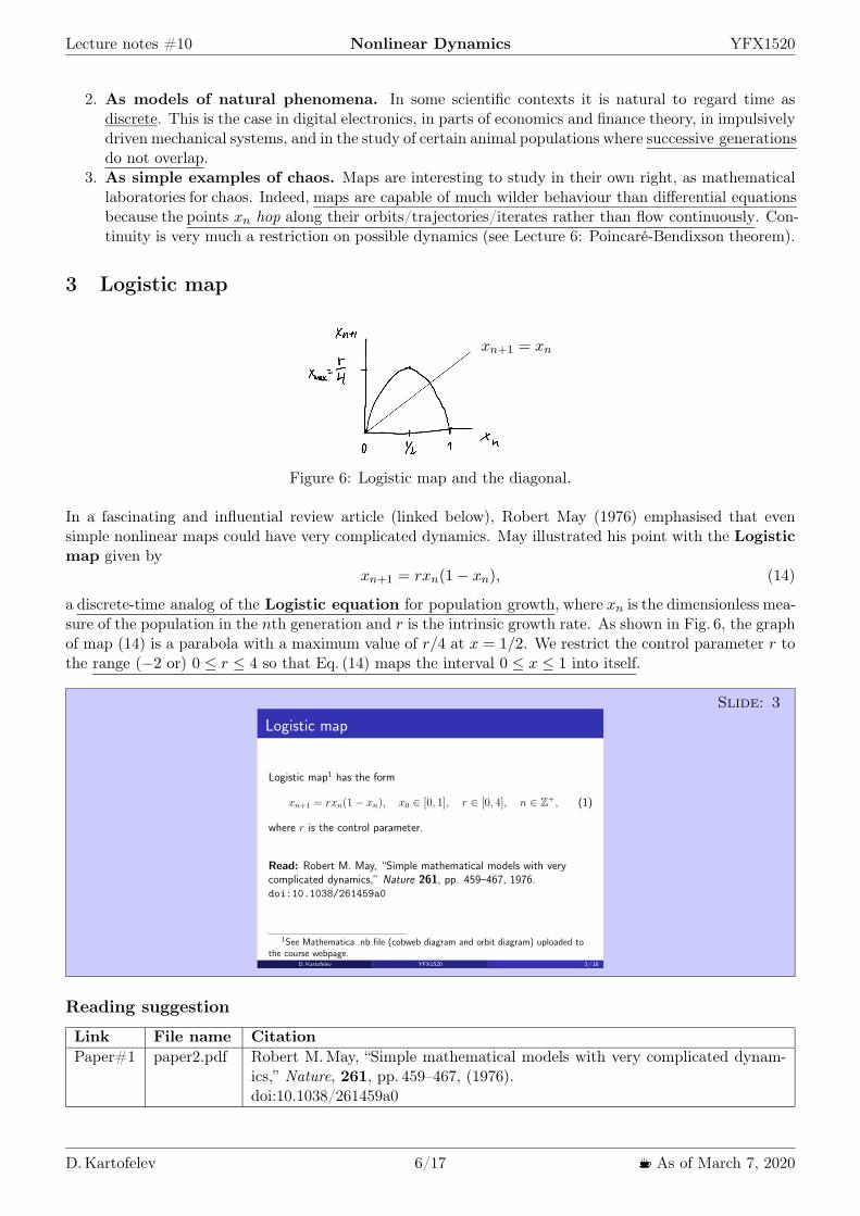
Lecture notes 10 Nonlinear Dynamics YFX1520
2 As models of natural phenomena In some scientific contexts it is natural to regard time asdiscrete This is the case in digital electronics in parts of economics and finance theory in impulsivelydriven mechanical systems and in the study of certain animal populations where successive generationsdo not overlap
3 As simple examples of chaos Maps are interesting to study in their own right as mathematicallaboratories for chaos Indeed maps are capable of much wilder behaviour than differential equationsbecause the points xn hop along their orbitstrajectoriesiterates rather than flow continuously Con-tinuity is very much a restriction on possible dynamics (see Lecture 6 Poincareacute-Bendixson theorem)
3 Logistic map
xn+1 = xn
Figure 6 Logistic map and the diagonal
In a fascinating and influential review article (linked below) Robert May (1976) emphasised that evensimple nonlinear maps could have very complicated dynamics May illustrated his point with the Logisticmap given by
xn+1 = rxn(1minus xn) (14)
a discrete-time analog of the Logistic equation for population growth where xn is the dimensionless mea-sure of the population in the nth generation and r is the intrinsic growth rate As shown in Fig 6 the graphof map (14) is a parabola with a maximum value of r4 at x = 12 We restrict the control parameter r tothe range (minus2 or) 0 le r le 4 so that Eq (14) maps the interval 0 le x le 1 into itself
Slide 3Logistic map
Logistic map1 has the form
xn+1 = rxn(1 xn) x0 2 [0 1] r 2 [0 4] n 2 Z+ (1)
where r is the control parameter
Read Robert M May ldquoSimple mathematical models with verycomplicated dynamicsrdquo Nature 261 pp 459ndash467 1976doi101038261459a0
1See Mathematica nb file (cobweb diagram and orbit diagram) uploaded tothe course webpage
DKartofelev YFX1520 3 18
Reading suggestion
Link File name CitationPaper1 paper2pdf Robert M May ldquoSimple mathematical models with very complicated dynam-
icsrdquo Nature 261 pp 459ndash467 (1976)doi101038261459a0
D Kartofelev 617 1003211 As of March 7 2020
Lecture notes 10 Nonlinear Dynamics YFX1520
31 Lyapunov exponent
The calculation of Lyapunov exponents of differential equations is not a trivial task In the case of maps itis much easier We remind that the positive Lyapunov exponent λ is a sign of chaos
Slides 4ndash6
Lyapunov exponent of Logistic map
Chaos is characterised by sensitive dependence on initialconditions If we take two close-by initial conditions say x0 andy0 = x0 + with 1 and iterate them under the map then thedicrarrerence between the two time series n = yn xn should growexponentially
|n| |0en| (2)
where is the Lyapunov exponent For maps this definition leads toa very simple way of measuring Lyapunov exponents Solving (2) for gives
=1
nln
n0
(3)
By definition n = fn(x0 + 0) fn(x0) Thus
=1
nln
fn(x0 + 0) fn(x0)
0
(4)
DKartofelev YFX1520 4 18
Lyapunov exponent of Logistic map
For small values of 0 the quantity inside the absolute value signs isjust the derivative of fn with respect to x evaluated at x = x0
=1
nln
dfn
dx
x=x0
(5)
Since fn(x) = f(f(f( f(x))) ) by the chain ruledfn
dx
x=x0
=f 0(fn1(x0)) middot f 0(fn2(x0)) middot middot f 0(x0)
= |f 0(xn1) middot f 0(xn2) middot middot f 0(x0)| =
n1Y
i=0
f 0(xi)
(6)
Our expression for the Lyapunov exponent becomes
=1
nln
n1Y
i=0
f 0(xi)
=1
n
n1X
i=0
ln |f 0(xi)| (7)
DKartofelev YFX1520 5 18
Lyapunov exponent of Logistic map
=1
nln
n1Y
i=0
f 0(xi)
=1
n
n1X
i=0
ln |f 0(xi)|
Lyapunov exponent is the large iterate n limit of this expression andso we have
= limn1
1
n
n1X
i=0
ln |f 0(xi)| (8)
This formula can be used to study Lyapunov exponent2 as a functionof control parameter r
(r) = limn1
1
n
n1X
i=0
ln |f 0(xi r)| (9)
2See Mathematica nb file uploaded to course webpageDKartofelev YFX1520 6 18
The obtained algorithm is used in the following numerical file to calculate the Lyapunov exponent of theLogistic map as a function of the growth rate r
Numerics cdf1 nb1Cobweb diagram and iterates of the (generalised) Lorenz map Lyapunov exponent λ(r) of the Logisticmap
-2 -1 0 1 2 3 4
-3
-2
-1
0
r
Figure 7 Lyapunov exponent of the Logistic map as a function of the growth rate r Calculation uses5000 iterations for every r value plotted
D Kartofelev 717 1003211 As of March 7 2020
Lecture notes 10 Nonlinear Dynamics YFX1520
32 Bifurcation analysis and period doubling bifurcation
Next letrsquos consider only the stable fixed point and stable period-p points as we incrementally increase thevalue of control parameter r ge 0 We do that in order to simplify our analysis and to save some lecturetime The stable fixed point (period-1 point) of Logistic map given by (14) and satisfying condition (2) is
f(xlowast) = xlowast rArr rxlowast(1minus xlowast) = xlowast | divide xlowast (15)
r(1minus xlowast) = 1 (16)
r minus rxlowast = 1 | divide r (17)
1minus xlowast =1
r (18)
xlowast = 1minus 1
r (19)
Additionally there are the trivial solutions xlowast = 0 and xlowast = 1 (for initial condition x0 = xlowast = 1 and forn gt 1 xn rarr xlowast = 0) Fixed point (19) is stable for |f prime(xlowast)| lt 1 Using map definition (14) we write
|f prime(xlowast)| =983055983055[rx(1minus x)]prime
983055983055x=xlowast = |r minus 2rxlowast| lt 1 (20)
Using condition (20) and for the trivial fixed point xlowast = 0 we get
|r minus 0| lt 1 (21)
|r| lt 1 (22)
The other trivial fixed point xlowast = 1 gives the same result
|r minus 2r| lt 1 (23)
|minus r| lt 1 (24)
Thus the fixed points xlowast = 0 and xlowast = 1 are stable for |plusmnr| lt 1 For the non-trivial fixed point xlowast = 1minus1rand for condition (20) we find 983055983055983055983055r minus 2r
9830611minus 1
r
983062983055983055983055983055 lt 1 (25)
|r minus 2r + 2| lt 1 (26)
|2minus r| lt 1 (27)
1 lt |r| lt 3 (28)
The fixed points xlowast = 1minus 1r exist and is stable for 1 lt |r| lt 3It seems that the found intervals (22) (24) and (28) excluded r = 1 (obviously it does not satisfy
|f prime(xlowast)| lt 1) Letrsquos find the value of the map slope |f prime(xlowast)| for r = 1 using (20) in the case of the trivialsolutions xlowast = 0
|f prime(xlowast)| = |1minus 0| = 1 (29)
xlowast = 1|f prime(xlowast)| = |1minus 2| = 1 (30)
and in the non-trivial case for xlowast = 1minus 1r = 1minus 1 = 0 Which should obviously generate the same result
|f prime(xlowast)| =9830559830559830559830551minus 2
9830611minus 1
1
983062983055983055983055983055 = |1minus 0| = 1 (31)
Below it will also be beneficial to know what happens for r = 3 the r value just after the interval (28)We consider the non-trivial fixed point xlowast = 1minus 1r and find the slope
|f prime(xlowast)| =9830559830559830559830553minus 2 middot 3
9830611minus 1
3
983062983055983055983055983055 = |3minus 4| = |minus 1| = 1 (32)
Usually slope |f prime(xlowast)| = 1 corresponds to the (period doubling or flip) bifurcation point Values r = 1and r = 3 are the bifurcation points Figure 8 shows the map positions of the fixed points and map slopes|f prime(xlowast)| evaluated at the non-trivial fixed point xlowast = 1minus 1r for r = 1 and r = 3
D Kartofelev 817 1003211 As of March 7 2020
Lecture notes 10 Nonlinear Dynamics YFX1520
Figure 8 (Left) Map slope at the fixed points xlowast = 1 minus 1r (same as the trivial case xlowast = 0) for r = 1(Right) Map slope at the fixed points xlowast = 1minus 1r for r = 3
The following interactive numerical file show the dynamics of Logistic map for 0 le |r| lt 1 and 1 lt |r| lt 3
Numerics cdf2 nb2Cobweb diagram of the Logistic map Orbit diagram of the Logistic map Period doubling and orbitdiagram
00 02 04 06 08 1000
02
04
06
08
10
xn
xn+1
0 5 10 15 2000
02
04
06
08
10
n
xn
00 02 04 06 08 1000
02
04
06
08
10
xn
xn+1
0 5 10 15 2000
02
04
06
08
10
n
xn
Figure 9 (Top-left) Cobweb diagram of the Logistic map shown for r = 098 lt 1 The fixed pointxlowast = 0 (Top-right) Map iterates corresponding to the cobweb diagram shown on the left (Bottom-left)Cobweb diagram of the Logistic map shown for interval 1 lt |r| lt 3 with r = 282 The fixed pointxlowast = 1minus 1r (Bottom-right) Map iterates corresponding to the cobweb diagram shown on the left
What happens for r ge 3 What happens after the period doubling or flip bifurcation at r = 3 Thename ldquofliprdquo refers to the fact that the map trajectories start to flip between two values mdash period-2 pointsin period-2 orbit Letrsquos check the dynamics using a computer
Numerics cdf2 nb2Cobweb diagram of the Logistic map Orbit diagram of the Logistic map Period doubling and orbitdiagramAfter the initial transient behaviour has decayed the dynamics of the map settles to a stableperiod-2 orbit It can be showed that period-2 orbits exist for 3 le r lt 1 +
radic6
D Kartofelev 917 1003211 As of March 7 2020
Lecture notes 10 Nonlinear Dynamics YFX1520
00 02 04 06 08 1000
02
04
06
08
10
xn
xn+1
0 5 10 15 20 25 3000
02
04
06
08
10
n
xn
Figure 10 (Left) Cobweb diagram of the Logistic map shown for r = 319 ge 3 featuring the stableperiod-2 point (Right) Map iterates corresponding to the cobweb diagram shown on the left
Letrsquos try to think about this outcome some more
Slides 7ndash9
Logistic map period-2 window
Period-2 window for 3 r lt 1 +p6
Figure Logistic map where r = 318 and x0 = 035 Fixed points (fps)in the case where r lt 3 are shown with the grey bullets Period-2 pointsof f(x) map for r 3 are shown with the blue bullets The fixed points off2(x) map for r 3 are shown with the red bullets
DKartofelev YFX1520 7 18
Logistic map period-2 window
Period-2 window for 3 r lt 1 +p6
(f(p) = rp(1 p) = q
f(q) = rq(1 q) = p(10)
where period-2 point values p and q are the fps of f(x) map
On the other hand it also holds(f(p) = f(f(q)) f 2(q) = r[rq(1 q)][1 (rq(1 q))] = q
f(q) = f(f(p)) f 2(p) = r[rp(1 p)][1 (rp(1 p))] = p)
(11)) f 2(x) = r[rx(1 x)][1 (rx(1 x))] = x (12)
where period-2 point values p and q are the fps of f 2(x) map
DKartofelev YFX1520 8 18
If you want to study the dynamics of the attractors of second iterate map f2 analytically consider oneof the equations in (11 slide numbering) The fourth order polynomial defined by Eq (7)
r[rx(1minus x)][1minus (rx(1minus x))] = x (33)
minus r3x4 + 2r3x3 minus r2(1 + r)x2 + r2x = x (34)
Intersections between the graph of second iterate map f2 and the diagonal correspond to the solutionsof f2(x) = x (34)
Stability of fps of f 2map in period-2 orbit
We need to know the slopes of period-2 points(f(p) = rp(1 p) = q
f(q) = rq(1 q) = p
According to the chain rule it holds that
(f 2(x))0 (f(f(x))0 = f 0(f(x)) middot f 0(x) (13)
In our case
(f 2(p))0 = f 0(f(p)) middot f 0(p) = f 0(q) middot f 0(p)
(f 2(q))0 = f 0(f(q)) middot f 0(q) = f 0(p) middot f 0(q)
)) (f 2(p))0 = (f 2(q))0
(14)Above follows from the commutative property of multiplication
DKartofelev YFX1520 9 18
D Kartofelev 1017 1003211 As of March 7 2020
Lecture notes 10 Nonlinear Dynamics YFX1520
The slopes of map f2 at its fixed points p and q are equal and they are the products of map f slopesat its respective period-2 points
What happens for r ge 1 +radic6 Once again we use a computer
Numerics cdf2 nb2Cobweb diagram of the Logistic map Orbit diagram of the Logistic map Period doubling and orbitdiagram
A period-4 orbit has emerged It can be shown that period-4 orbits exist for 1 +radic6 le r lt 354409
00 02 04 06 08 1000
02
04
06
08
10
xn
xn+1
0 5 10 15 20 25 3000
02
04
06
08
10
n
xn
Figure 11 (Left) Cobweb diagram of the Logistic map shown for r = 3535 ge 1 +radic6 featuring the
stable period-4 point The blue graph shows fourth iterate map f4 (Right) Map iterates correspondingto the cobweb diagram of map f shown on the left
Figure 12 counts the period-4 pointsiterates in the period-4 orbit of the Logistic map Compare Fig 12 toFig 5
Figure 12 Period-4 orbit in the Logistic map
What have we seen so far As we have incrementally increased the value of control parameter r theperiods of the fixed points have increased as well mdash from period-1 to period-2 and finally to period-4The period is clearly doubling This type of bifurcation is called the period doubling bifurca-tion Further period-doublings to orbits of period-8 -16 -32 etc occur as r increases Specifically letrn denote the value of r where a stable 2n-orbit first appears Then computer experiments reveal that
D Kartofelev 1117 1003211 As of March 7 2020
Lecture notes 10 Nonlinear Dynamics YFX1520
Slide 10
Logistic map period doubling
Even number periods
rn ndash bifurcation point onset of stable period-2n orbit
r1 = 30 period-2r2 = 1 +
p6 344949 period-4
r3 354409 period-8r4 356441 period-16r5 356875 period-32r6 356969 period-64
r1 3569946 period-21
r1 ndash onset of chaos (the accumulation point)
= limn1
rn1 rn2
rn rn1 4669201609 (15)
DKartofelev YFX1520 10 18
Note that the successive bifurcations come faster and faster Ultimately the rn converge toa limiting value rinfin The convergence is (essentially) geometric (itrsquos geometric near rinfin) in the limitof large n the distance between successive transitions shrinks by a constant factor of δ This ratio iscalled the Feigenbaum constant After the accumulation point r gt rinfin the dynamics becomeschaotic as wersquoll see below
33 Orbit diagram
The orbit diagram is also called the fig tree diagram (Feigenbaum in German means ldquofig treerdquo) or (in-correctly) the Feigenbaum diagram You might guess that the system would become more and morechaotic for r gt rinfin as r increases but in fact the dynamics are more subtle than that To see the long-termbehaviour for all values of r at once we plot the orbit diagram a special kind of bifurcation diagramOrbit diagram plots the systemrsquos attractor (stable fixed points and stable period-p points) as a function ofcontrol parameter r
To generate the orbit diagram for yourself yoursquoll need to write a computer program with two loops Firstchoose a value of r Then generate an orbit starting from some random initial condition x0 Iterate for 300cycles or so to allow the system to settle down to its eventual stable behaviour Once the transients havedecayed plot many points say x301 x900 above that r Then move to an adjacent value of r and repeateventually sweeping across the whole diagram
The following interactive numerical file shows the orbit diagram for the Logistic map
Numerics cdf2 nb2Cobweb diagram of the Logistic map Orbit diagram of the Logistic map Period doubling and orbitdiagram
The connection between the cobweb diagram orbit diagram and the Lyapunov exponent is shown in theinteractive numerical file linked below
Numerics cdf3 nb3Logistic map cobweb diagram orbit diagram and map iterates Lyapunov exponent
D Kartofelev 1217 1003211 As of March 7 2020
Lecture notes 10 Nonlinear Dynamics YFX1520
Slides 11 12
Orbit diagram and period doubling
DKartofelev YFX1520 11 18
Zooming into the Logistic map self-similarity
No embedded video files in this pdf
DKartofelev YFX1520 12 18
The period doubling is driven by the subsequent flip bifurcations or supercritical pitchforkbifurcations (if we use the nomenclature introduced in Lecture 2) The unstable fixed point andperiod-p points are omitted from the orbit diagram
Feigenbaum diagram shows both stable and unstable fixed points and period-p points or simplydiagram branches (not shown here)
The orbit diagram of the Logistic map features self-similarity In mathematics a self-similarobject is (exactly or) approximately similar to a part of itself ie the whole has the same shape orquality as one or more of its sub-parts
34 Tangent bifurcation and odd number period-p points
Can an odd number period appear in the Logistic map mdash eg period-3 point One of the most intriguingfeatures of the orbit diagram is the occurrence of periodic windows for r gt rinfin The period-3 windowthat occurs for 1 +
radic8 le r le 38415 is the most conspicuous Suddenly against a backdrop of chaos a
stable period-3 orbit appears out of the blueLetrsquos see if we can find the period-3 window of Logistic map using a computer
Numerics cdf2 nb2Cobweb diagram of the Logistic map Orbit diagram of the Logistic map Period doubling and orbitdiagram
The tangent bifurcation is a new type of bifurcation for us that occurs at r = 1 +radic8
00 02 04 06 08 1000
02
04
06
08
10
xn
xn+1
0 5 10 15 20 25 3000
02
04
06
08
10
n
xn
Figure 13 (Left) Period-3 orbit of map f can be found in the period-3 window Here showing thetrajectory for r = 383 (Right) Map iterates corresponding to the cobweb diagram of map f shownon the left
The mechanism responsible for the occurrence of the odd number periods-p points is shown in Fig 14The intersections between the graph of f3 shown in red and the diagonal correspond to solutions of
D Kartofelev 1317 1003211 As of March 7 2020
Lecture notes 10 Nonlinear Dynamics YFX1520
Figure 14 Period-3 orbit can be found in period-3 window of the orbit diagram
f3(x) = x There are eight solutions for r ge 1+radic8 six of interest to us are marked with the blue dots and
two imposters that are not genuine period-3 they are actually fixed points or period-1 points for whichf(xlowast) = xlowast The blue filled dots in Fig 14 correspond to a stable period-3 cycle note that the slope off3(x) is shallow at these points consistent with the stability of the cycle In contrast the slope exceeds 1at the cycle marked by the empty blue dots this period-3 orbit is therefore unstable
Now suppose we decrease r toward the chaotic regime r lt 1+radic8 Then the red graph in Fig 14 changes
shape mdash the hill moves down and the valleys rise up The curve therefore moves towards the diagonalFigure 14 shows that when r = 1 +
radic8 the six blue intersections have merged to form three black filled
period-3 points by becoming tangent to the diagonal At this critical value of r the stable and unstableperiod-3 cycles coalesce and annihilate in a tangent bifurcation This transition defines the beginning ofthe periodic period-3 window
All odd number periods will also undergo the period doubling This means that all number periods [1infin)are eventually represented in the orbit diagram
Figure 14 also explains the self-similarity present in the orbit diagram as shown on Slide 12 for differentscales of magnification The peaks and valley of map f3 are smaller distorted copies of the original mapf Thus the local dynamics of the cobweb trajectories for map f3 must be similar to the dynamics of theoriginal map f
Slide 13
Intermittency3and period-3 window
Transient chaos and intermittency in dynamical systemsTangent bifurcation occurs at r = 1 +
p8 38284 (period-3 orbit)
50 100 150n
02
04
06
08
10xn
Iterates of Logistic map shown for r = 38282 and x0 = 015
3See Mathematica nb file uploaded to course webpageDKartofelev YFX1520 13 18
The dynamics closely related to the tangent bifurcation is intermittency Logistic map exhibitsintermittent chaos for r values just before the period-3 window
D Kartofelev 1417 1003211 As of March 7 2020
Lecture notes 10 Nonlinear Dynamics YFX1520
Numerics cdf4 nb4Period-3 window and intermittency in the Logistic map (iterates xn)
4 Sine map and universality of period doubling
It can be shown that in all unimodal maps same dynamics of period doubling occurs For example weconsider the sine map
Slide 14
Universality of period doubling in unimodal maps
1-D sine map4 The sine map has the form
xn+1 = r sin(xn) x0 2 [0 1] r 2 [0 1] n 2 Z+ (16)
where r is the control parameter
Read Mitchell J Feigenbaum ldquoQuantitative universality for a classof nonlinear transformationsrdquo Journal of Statistical Physics 19(1)pp 25ndash52 1978 doi101007BF01020332
Read Mitchell J Feigenbaum ldquoUniversal behavior in nonlinearsystemsrdquo Physica D Nonlinear Phenomena 7(1ndash3) pp 16ndash391983 doi1010160167-2789(83)90112-4
4See Mathematica nb file (cobweb diagram and orbit diagram) uploaded tothe course webpage
DKartofelev YFX1520 14 18
The graph of the sine map has the same basic shape as the graph of the Logistic map Both curvesare smooth concave down and have a single maximum Such maps are called unimodal
Sine is also a transcendental function opposed to an algebraic function as is the polynomial thatdescribes the Logistic map A transcendental function is an analytic function that does not satisfy apolynomial equation In other words a transcendental function ldquotranscendsrdquo algebra in that it cannotbe expressed in terms of a finite sequence of the algebraic operations of addition multiplication androot extraction
The transcendental nature of the sine map must makes the underlying higher-dimensional physicsrepresented by the sine map fundamentally different from eg the three-dimensional Lorenz flowsampled by Lorenz map
Letrsquos study the dynamics of the sine map using a computer
Numerics cdf5 nb5The sine map iterates cobweb and orbit diagrams (xn isin [0 1])
Numerics cdf6 nb6The sine map iterates cobweb and orbit diagrams (xn isin [minus1 1])
The dynamics is surprisingly similar to the dynamics of the Logistic map Mitchell J Feigenbaumwas first to discover the quantitative laws that are independent of unimodal map functions f Bythat we mean that the algebraic form of f(x) is irrelevant only its overall shape matters
D Kartofelev 1517 1003211 As of March 7 2020
Lecture notes 10 Nonlinear Dynamics YFX1520
Slide 151-D unimodal maps and Feigenbaum constants
= limn1
n1
n= lim
n1
rn1 rn2
rn rn1 4669201609 (17)
crarr = limn1
dn1
dn 2502907875 (18)
DKartofelev YFX1520 15 18
Here xm = max f(x) is the maximum of the map graph The Feigenbaum constants are valid up tothe onset of chaos at rinfin and inside each periodic window for r gt rinfin
In addition to scaling law in control parameter r direction shown earlier Feigenbaum also foundscaling law for the vertical x-direction of the orbit diagram The Feigenbaum constants are uni-versal the same convergence rate appears no matter what unimodal map is iterated They are newmathematical constants as basic to period doubling as π is to circles
Reading suggestion
Link File name CitationPaper2 paper3pdf Mitchell J Feigenbaum ldquoQuantitative universality for a class of nonlinear trans-
formationsrdquo Journal of Statistical Physics 19(1) pp 25ndash52 (1978)doi101007BF01020332
Paper3 paper4pdf Mitchell J Feigenbaum ldquoUniversal behavior in nonlinear systemsrdquo Physica DNonlinear Phenomena 7(1ndash3) pp 16ndash39 (1983)doi1010160167-2789(83)90112-4
5 Universal route to chaos
We showed that the qualitative dynamics of the Logistic and sine maps are identical They both undergoperiod doubling routes to chaos followed by periodic windows interwoven with chaotic bandsEven more remarkably the periodic windows occur in the same order and with the same relative sizes Forinstance the period-3 window is the largest in both cases and the next largest windows preceding it areperiod-5 and period-6 But there are quantitative differences For instance the period doubling bifurcationsoccur later (for greater parameter r value) in the Logistic map and the periodic windows are thinner
Turns out that the onset of chaos via period doubling is predominant in nature and in artificial chaoticsystems Feigenbaum constants have real predictive power in various scientific applications The perioddoubling bifurcation is the ldquorouterdquo taken by nonlinear systems to reach chaotic solution Interm of the bifurcations introduced in Lecture 2 the period doubling bifurcation can also be seen as a seriesof subsequentsucceeding supercritical pitchfork bifurcations see Slide 11
Revision questions
1 What is cobweb diagram2 What is recurrence map or recurrence relation3 What is 1-D map4 How to find fixed points of 1-D maps5 What is Lorenz map
D Kartofelev 1617 1003211 As of March 7 2020
Lecture notes 10 Nonlinear Dynamics YFX1520
6 What is Logistic map7 What is sine map8 What is period doubling9 What is period doubling bifurcation
10 What is tangent bifurcation11 Do odd number periods (period-p orbits) exist in chaotic systems12 Do even number periods (period-p orbits) exist in chaotic systems13 Can maps produce transient chaos14 Can maps produce intermittency15 Can maps produce intermittent chaos16 What is orbit diagram (or Feigenbaum diagram)17 What are Feigenbaum constants
D Kartofelev 1717 1003211 As of March 7 2020
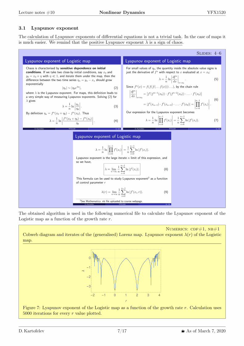
Lecture notes 10 Nonlinear Dynamics YFX1520
31 Lyapunov exponent
The calculation of Lyapunov exponents of differential equations is not a trivial task In the case of maps itis much easier We remind that the positive Lyapunov exponent λ is a sign of chaos
Slides 4ndash6
Lyapunov exponent of Logistic map
Chaos is characterised by sensitive dependence on initialconditions If we take two close-by initial conditions say x0 andy0 = x0 + with 1 and iterate them under the map then thedicrarrerence between the two time series n = yn xn should growexponentially
|n| |0en| (2)
where is the Lyapunov exponent For maps this definition leads toa very simple way of measuring Lyapunov exponents Solving (2) for gives
=1
nln
n0
(3)
By definition n = fn(x0 + 0) fn(x0) Thus
=1
nln
fn(x0 + 0) fn(x0)
0
(4)
DKartofelev YFX1520 4 18
Lyapunov exponent of Logistic map
For small values of 0 the quantity inside the absolute value signs isjust the derivative of fn with respect to x evaluated at x = x0
=1
nln
dfn
dx
x=x0
(5)
Since fn(x) = f(f(f( f(x))) ) by the chain ruledfn
dx
x=x0
=f 0(fn1(x0)) middot f 0(fn2(x0)) middot middot f 0(x0)
= |f 0(xn1) middot f 0(xn2) middot middot f 0(x0)| =
n1Y
i=0
f 0(xi)
(6)
Our expression for the Lyapunov exponent becomes
=1
nln
n1Y
i=0
f 0(xi)
=1
n
n1X
i=0
ln |f 0(xi)| (7)
DKartofelev YFX1520 5 18
Lyapunov exponent of Logistic map
=1
nln
n1Y
i=0
f 0(xi)
=1
n
n1X
i=0
ln |f 0(xi)|
Lyapunov exponent is the large iterate n limit of this expression andso we have
= limn1
1
n
n1X
i=0
ln |f 0(xi)| (8)
This formula can be used to study Lyapunov exponent2 as a functionof control parameter r
(r) = limn1
1
n
n1X
i=0
ln |f 0(xi r)| (9)
2See Mathematica nb file uploaded to course webpageDKartofelev YFX1520 6 18
The obtained algorithm is used in the following numerical file to calculate the Lyapunov exponent of theLogistic map as a function of the growth rate r
Numerics cdf1 nb1Cobweb diagram and iterates of the (generalised) Lorenz map Lyapunov exponent λ(r) of the Logisticmap
-2 -1 0 1 2 3 4
-3
-2
-1
0
r
Figure 7 Lyapunov exponent of the Logistic map as a function of the growth rate r Calculation uses5000 iterations for every r value plotted
D Kartofelev 717 1003211 As of March 7 2020
Lecture notes 10 Nonlinear Dynamics YFX1520
32 Bifurcation analysis and period doubling bifurcation
Next letrsquos consider only the stable fixed point and stable period-p points as we incrementally increase thevalue of control parameter r ge 0 We do that in order to simplify our analysis and to save some lecturetime The stable fixed point (period-1 point) of Logistic map given by (14) and satisfying condition (2) is
f(xlowast) = xlowast rArr rxlowast(1minus xlowast) = xlowast | divide xlowast (15)
r(1minus xlowast) = 1 (16)
r minus rxlowast = 1 | divide r (17)
1minus xlowast =1
r (18)
xlowast = 1minus 1
r (19)
Additionally there are the trivial solutions xlowast = 0 and xlowast = 1 (for initial condition x0 = xlowast = 1 and forn gt 1 xn rarr xlowast = 0) Fixed point (19) is stable for |f prime(xlowast)| lt 1 Using map definition (14) we write
|f prime(xlowast)| =983055983055[rx(1minus x)]prime
983055983055x=xlowast = |r minus 2rxlowast| lt 1 (20)
Using condition (20) and for the trivial fixed point xlowast = 0 we get
|r minus 0| lt 1 (21)
|r| lt 1 (22)
The other trivial fixed point xlowast = 1 gives the same result
|r minus 2r| lt 1 (23)
|minus r| lt 1 (24)
Thus the fixed points xlowast = 0 and xlowast = 1 are stable for |plusmnr| lt 1 For the non-trivial fixed point xlowast = 1minus1rand for condition (20) we find 983055983055983055983055r minus 2r
9830611minus 1
r
983062983055983055983055983055 lt 1 (25)
|r minus 2r + 2| lt 1 (26)
|2minus r| lt 1 (27)
1 lt |r| lt 3 (28)
The fixed points xlowast = 1minus 1r exist and is stable for 1 lt |r| lt 3It seems that the found intervals (22) (24) and (28) excluded r = 1 (obviously it does not satisfy
|f prime(xlowast)| lt 1) Letrsquos find the value of the map slope |f prime(xlowast)| for r = 1 using (20) in the case of the trivialsolutions xlowast = 0
|f prime(xlowast)| = |1minus 0| = 1 (29)
xlowast = 1|f prime(xlowast)| = |1minus 2| = 1 (30)
and in the non-trivial case for xlowast = 1minus 1r = 1minus 1 = 0 Which should obviously generate the same result
|f prime(xlowast)| =9830559830559830559830551minus 2
9830611minus 1
1
983062983055983055983055983055 = |1minus 0| = 1 (31)
Below it will also be beneficial to know what happens for r = 3 the r value just after the interval (28)We consider the non-trivial fixed point xlowast = 1minus 1r and find the slope
|f prime(xlowast)| =9830559830559830559830553minus 2 middot 3
9830611minus 1
3
983062983055983055983055983055 = |3minus 4| = |minus 1| = 1 (32)
Usually slope |f prime(xlowast)| = 1 corresponds to the (period doubling or flip) bifurcation point Values r = 1and r = 3 are the bifurcation points Figure 8 shows the map positions of the fixed points and map slopes|f prime(xlowast)| evaluated at the non-trivial fixed point xlowast = 1minus 1r for r = 1 and r = 3
D Kartofelev 817 1003211 As of March 7 2020
Lecture notes 10 Nonlinear Dynamics YFX1520
Figure 8 (Left) Map slope at the fixed points xlowast = 1 minus 1r (same as the trivial case xlowast = 0) for r = 1(Right) Map slope at the fixed points xlowast = 1minus 1r for r = 3
The following interactive numerical file show the dynamics of Logistic map for 0 le |r| lt 1 and 1 lt |r| lt 3
Numerics cdf2 nb2Cobweb diagram of the Logistic map Orbit diagram of the Logistic map Period doubling and orbitdiagram
00 02 04 06 08 1000
02
04
06
08
10
xn
xn+1
0 5 10 15 2000
02
04
06
08
10
n
xn
00 02 04 06 08 1000
02
04
06
08
10
xn
xn+1
0 5 10 15 2000
02
04
06
08
10
n
xn
Figure 9 (Top-left) Cobweb diagram of the Logistic map shown for r = 098 lt 1 The fixed pointxlowast = 0 (Top-right) Map iterates corresponding to the cobweb diagram shown on the left (Bottom-left)Cobweb diagram of the Logistic map shown for interval 1 lt |r| lt 3 with r = 282 The fixed pointxlowast = 1minus 1r (Bottom-right) Map iterates corresponding to the cobweb diagram shown on the left
What happens for r ge 3 What happens after the period doubling or flip bifurcation at r = 3 Thename ldquofliprdquo refers to the fact that the map trajectories start to flip between two values mdash period-2 pointsin period-2 orbit Letrsquos check the dynamics using a computer
Numerics cdf2 nb2Cobweb diagram of the Logistic map Orbit diagram of the Logistic map Period doubling and orbitdiagramAfter the initial transient behaviour has decayed the dynamics of the map settles to a stableperiod-2 orbit It can be showed that period-2 orbits exist for 3 le r lt 1 +
radic6
D Kartofelev 917 1003211 As of March 7 2020
Lecture notes 10 Nonlinear Dynamics YFX1520
00 02 04 06 08 1000
02
04
06
08
10
xn
xn+1
0 5 10 15 20 25 3000
02
04
06
08
10
n
xn
Figure 10 (Left) Cobweb diagram of the Logistic map shown for r = 319 ge 3 featuring the stableperiod-2 point (Right) Map iterates corresponding to the cobweb diagram shown on the left
Letrsquos try to think about this outcome some more
Slides 7ndash9
Logistic map period-2 window
Period-2 window for 3 r lt 1 +p6
Figure Logistic map where r = 318 and x0 = 035 Fixed points (fps)in the case where r lt 3 are shown with the grey bullets Period-2 pointsof f(x) map for r 3 are shown with the blue bullets The fixed points off2(x) map for r 3 are shown with the red bullets
DKartofelev YFX1520 7 18
Logistic map period-2 window
Period-2 window for 3 r lt 1 +p6
(f(p) = rp(1 p) = q
f(q) = rq(1 q) = p(10)
where period-2 point values p and q are the fps of f(x) map
On the other hand it also holds(f(p) = f(f(q)) f 2(q) = r[rq(1 q)][1 (rq(1 q))] = q
f(q) = f(f(p)) f 2(p) = r[rp(1 p)][1 (rp(1 p))] = p)
(11)) f 2(x) = r[rx(1 x)][1 (rx(1 x))] = x (12)
where period-2 point values p and q are the fps of f 2(x) map
DKartofelev YFX1520 8 18
If you want to study the dynamics of the attractors of second iterate map f2 analytically consider oneof the equations in (11 slide numbering) The fourth order polynomial defined by Eq (7)
r[rx(1minus x)][1minus (rx(1minus x))] = x (33)
minus r3x4 + 2r3x3 minus r2(1 + r)x2 + r2x = x (34)
Intersections between the graph of second iterate map f2 and the diagonal correspond to the solutionsof f2(x) = x (34)
Stability of fps of f 2map in period-2 orbit
We need to know the slopes of period-2 points(f(p) = rp(1 p) = q
f(q) = rq(1 q) = p
According to the chain rule it holds that
(f 2(x))0 (f(f(x))0 = f 0(f(x)) middot f 0(x) (13)
In our case
(f 2(p))0 = f 0(f(p)) middot f 0(p) = f 0(q) middot f 0(p)
(f 2(q))0 = f 0(f(q)) middot f 0(q) = f 0(p) middot f 0(q)
)) (f 2(p))0 = (f 2(q))0
(14)Above follows from the commutative property of multiplication
DKartofelev YFX1520 9 18
D Kartofelev 1017 1003211 As of March 7 2020
Lecture notes 10 Nonlinear Dynamics YFX1520
The slopes of map f2 at its fixed points p and q are equal and they are the products of map f slopesat its respective period-2 points
What happens for r ge 1 +radic6 Once again we use a computer
Numerics cdf2 nb2Cobweb diagram of the Logistic map Orbit diagram of the Logistic map Period doubling and orbitdiagram
A period-4 orbit has emerged It can be shown that period-4 orbits exist for 1 +radic6 le r lt 354409
00 02 04 06 08 1000
02
04
06
08
10
xn
xn+1
0 5 10 15 20 25 3000
02
04
06
08
10
n
xn
Figure 11 (Left) Cobweb diagram of the Logistic map shown for r = 3535 ge 1 +radic6 featuring the
stable period-4 point The blue graph shows fourth iterate map f4 (Right) Map iterates correspondingto the cobweb diagram of map f shown on the left
Figure 12 counts the period-4 pointsiterates in the period-4 orbit of the Logistic map Compare Fig 12 toFig 5
Figure 12 Period-4 orbit in the Logistic map
What have we seen so far As we have incrementally increased the value of control parameter r theperiods of the fixed points have increased as well mdash from period-1 to period-2 and finally to period-4The period is clearly doubling This type of bifurcation is called the period doubling bifurca-tion Further period-doublings to orbits of period-8 -16 -32 etc occur as r increases Specifically letrn denote the value of r where a stable 2n-orbit first appears Then computer experiments reveal that
D Kartofelev 1117 1003211 As of March 7 2020
Lecture notes 10 Nonlinear Dynamics YFX1520
Slide 10
Logistic map period doubling
Even number periods
rn ndash bifurcation point onset of stable period-2n orbit
r1 = 30 period-2r2 = 1 +
p6 344949 period-4
r3 354409 period-8r4 356441 period-16r5 356875 period-32r6 356969 period-64
r1 3569946 period-21
r1 ndash onset of chaos (the accumulation point)
= limn1
rn1 rn2
rn rn1 4669201609 (15)
DKartofelev YFX1520 10 18
Note that the successive bifurcations come faster and faster Ultimately the rn converge toa limiting value rinfin The convergence is (essentially) geometric (itrsquos geometric near rinfin) in the limitof large n the distance between successive transitions shrinks by a constant factor of δ This ratio iscalled the Feigenbaum constant After the accumulation point r gt rinfin the dynamics becomeschaotic as wersquoll see below
33 Orbit diagram
The orbit diagram is also called the fig tree diagram (Feigenbaum in German means ldquofig treerdquo) or (in-correctly) the Feigenbaum diagram You might guess that the system would become more and morechaotic for r gt rinfin as r increases but in fact the dynamics are more subtle than that To see the long-termbehaviour for all values of r at once we plot the orbit diagram a special kind of bifurcation diagramOrbit diagram plots the systemrsquos attractor (stable fixed points and stable period-p points) as a function ofcontrol parameter r
To generate the orbit diagram for yourself yoursquoll need to write a computer program with two loops Firstchoose a value of r Then generate an orbit starting from some random initial condition x0 Iterate for 300cycles or so to allow the system to settle down to its eventual stable behaviour Once the transients havedecayed plot many points say x301 x900 above that r Then move to an adjacent value of r and repeateventually sweeping across the whole diagram
The following interactive numerical file shows the orbit diagram for the Logistic map
Numerics cdf2 nb2Cobweb diagram of the Logistic map Orbit diagram of the Logistic map Period doubling and orbitdiagram
The connection between the cobweb diagram orbit diagram and the Lyapunov exponent is shown in theinteractive numerical file linked below
Numerics cdf3 nb3Logistic map cobweb diagram orbit diagram and map iterates Lyapunov exponent
D Kartofelev 1217 1003211 As of March 7 2020
Lecture notes 10 Nonlinear Dynamics YFX1520
Slides 11 12
Orbit diagram and period doubling
DKartofelev YFX1520 11 18
Zooming into the Logistic map self-similarity
No embedded video files in this pdf
DKartofelev YFX1520 12 18
The period doubling is driven by the subsequent flip bifurcations or supercritical pitchforkbifurcations (if we use the nomenclature introduced in Lecture 2) The unstable fixed point andperiod-p points are omitted from the orbit diagram
Feigenbaum diagram shows both stable and unstable fixed points and period-p points or simplydiagram branches (not shown here)
The orbit diagram of the Logistic map features self-similarity In mathematics a self-similarobject is (exactly or) approximately similar to a part of itself ie the whole has the same shape orquality as one or more of its sub-parts
34 Tangent bifurcation and odd number period-p points
Can an odd number period appear in the Logistic map mdash eg period-3 point One of the most intriguingfeatures of the orbit diagram is the occurrence of periodic windows for r gt rinfin The period-3 windowthat occurs for 1 +
radic8 le r le 38415 is the most conspicuous Suddenly against a backdrop of chaos a
stable period-3 orbit appears out of the blueLetrsquos see if we can find the period-3 window of Logistic map using a computer
Numerics cdf2 nb2Cobweb diagram of the Logistic map Orbit diagram of the Logistic map Period doubling and orbitdiagram
The tangent bifurcation is a new type of bifurcation for us that occurs at r = 1 +radic8
00 02 04 06 08 1000
02
04
06
08
10
xn
xn+1
0 5 10 15 20 25 3000
02
04
06
08
10
n
xn
Figure 13 (Left) Period-3 orbit of map f can be found in the period-3 window Here showing thetrajectory for r = 383 (Right) Map iterates corresponding to the cobweb diagram of map f shownon the left
The mechanism responsible for the occurrence of the odd number periods-p points is shown in Fig 14The intersections between the graph of f3 shown in red and the diagonal correspond to solutions of
D Kartofelev 1317 1003211 As of March 7 2020
Lecture notes 10 Nonlinear Dynamics YFX1520
Figure 14 Period-3 orbit can be found in period-3 window of the orbit diagram
f3(x) = x There are eight solutions for r ge 1+radic8 six of interest to us are marked with the blue dots and
two imposters that are not genuine period-3 they are actually fixed points or period-1 points for whichf(xlowast) = xlowast The blue filled dots in Fig 14 correspond to a stable period-3 cycle note that the slope off3(x) is shallow at these points consistent with the stability of the cycle In contrast the slope exceeds 1at the cycle marked by the empty blue dots this period-3 orbit is therefore unstable
Now suppose we decrease r toward the chaotic regime r lt 1+radic8 Then the red graph in Fig 14 changes
shape mdash the hill moves down and the valleys rise up The curve therefore moves towards the diagonalFigure 14 shows that when r = 1 +
radic8 the six blue intersections have merged to form three black filled
period-3 points by becoming tangent to the diagonal At this critical value of r the stable and unstableperiod-3 cycles coalesce and annihilate in a tangent bifurcation This transition defines the beginning ofthe periodic period-3 window
All odd number periods will also undergo the period doubling This means that all number periods [1infin)are eventually represented in the orbit diagram
Figure 14 also explains the self-similarity present in the orbit diagram as shown on Slide 12 for differentscales of magnification The peaks and valley of map f3 are smaller distorted copies of the original mapf Thus the local dynamics of the cobweb trajectories for map f3 must be similar to the dynamics of theoriginal map f
Slide 13
Intermittency3and period-3 window
Transient chaos and intermittency in dynamical systemsTangent bifurcation occurs at r = 1 +
p8 38284 (period-3 orbit)
50 100 150n
02
04
06
08
10xn
Iterates of Logistic map shown for r = 38282 and x0 = 015
3See Mathematica nb file uploaded to course webpageDKartofelev YFX1520 13 18
The dynamics closely related to the tangent bifurcation is intermittency Logistic map exhibitsintermittent chaos for r values just before the period-3 window
D Kartofelev 1417 1003211 As of March 7 2020
Lecture notes 10 Nonlinear Dynamics YFX1520
Numerics cdf4 nb4Period-3 window and intermittency in the Logistic map (iterates xn)
4 Sine map and universality of period doubling
It can be shown that in all unimodal maps same dynamics of period doubling occurs For example weconsider the sine map
Slide 14
Universality of period doubling in unimodal maps
1-D sine map4 The sine map has the form
xn+1 = r sin(xn) x0 2 [0 1] r 2 [0 1] n 2 Z+ (16)
where r is the control parameter
Read Mitchell J Feigenbaum ldquoQuantitative universality for a classof nonlinear transformationsrdquo Journal of Statistical Physics 19(1)pp 25ndash52 1978 doi101007BF01020332
Read Mitchell J Feigenbaum ldquoUniversal behavior in nonlinearsystemsrdquo Physica D Nonlinear Phenomena 7(1ndash3) pp 16ndash391983 doi1010160167-2789(83)90112-4
4See Mathematica nb file (cobweb diagram and orbit diagram) uploaded tothe course webpage
DKartofelev YFX1520 14 18
The graph of the sine map has the same basic shape as the graph of the Logistic map Both curvesare smooth concave down and have a single maximum Such maps are called unimodal
Sine is also a transcendental function opposed to an algebraic function as is the polynomial thatdescribes the Logistic map A transcendental function is an analytic function that does not satisfy apolynomial equation In other words a transcendental function ldquotranscendsrdquo algebra in that it cannotbe expressed in terms of a finite sequence of the algebraic operations of addition multiplication androot extraction
The transcendental nature of the sine map must makes the underlying higher-dimensional physicsrepresented by the sine map fundamentally different from eg the three-dimensional Lorenz flowsampled by Lorenz map
Letrsquos study the dynamics of the sine map using a computer
Numerics cdf5 nb5The sine map iterates cobweb and orbit diagrams (xn isin [0 1])
Numerics cdf6 nb6The sine map iterates cobweb and orbit diagrams (xn isin [minus1 1])
The dynamics is surprisingly similar to the dynamics of the Logistic map Mitchell J Feigenbaumwas first to discover the quantitative laws that are independent of unimodal map functions f Bythat we mean that the algebraic form of f(x) is irrelevant only its overall shape matters
D Kartofelev 1517 1003211 As of March 7 2020
Lecture notes 10 Nonlinear Dynamics YFX1520
Slide 151-D unimodal maps and Feigenbaum constants
= limn1
n1
n= lim
n1
rn1 rn2
rn rn1 4669201609 (17)
crarr = limn1
dn1
dn 2502907875 (18)
DKartofelev YFX1520 15 18
Here xm = max f(x) is the maximum of the map graph The Feigenbaum constants are valid up tothe onset of chaos at rinfin and inside each periodic window for r gt rinfin
In addition to scaling law in control parameter r direction shown earlier Feigenbaum also foundscaling law for the vertical x-direction of the orbit diagram The Feigenbaum constants are uni-versal the same convergence rate appears no matter what unimodal map is iterated They are newmathematical constants as basic to period doubling as π is to circles
Reading suggestion
Link File name CitationPaper2 paper3pdf Mitchell J Feigenbaum ldquoQuantitative universality for a class of nonlinear trans-
formationsrdquo Journal of Statistical Physics 19(1) pp 25ndash52 (1978)doi101007BF01020332
Paper3 paper4pdf Mitchell J Feigenbaum ldquoUniversal behavior in nonlinear systemsrdquo Physica DNonlinear Phenomena 7(1ndash3) pp 16ndash39 (1983)doi1010160167-2789(83)90112-4
5 Universal route to chaos
We showed that the qualitative dynamics of the Logistic and sine maps are identical They both undergoperiod doubling routes to chaos followed by periodic windows interwoven with chaotic bandsEven more remarkably the periodic windows occur in the same order and with the same relative sizes Forinstance the period-3 window is the largest in both cases and the next largest windows preceding it areperiod-5 and period-6 But there are quantitative differences For instance the period doubling bifurcationsoccur later (for greater parameter r value) in the Logistic map and the periodic windows are thinner
Turns out that the onset of chaos via period doubling is predominant in nature and in artificial chaoticsystems Feigenbaum constants have real predictive power in various scientific applications The perioddoubling bifurcation is the ldquorouterdquo taken by nonlinear systems to reach chaotic solution Interm of the bifurcations introduced in Lecture 2 the period doubling bifurcation can also be seen as a seriesof subsequentsucceeding supercritical pitchfork bifurcations see Slide 11
Revision questions
1 What is cobweb diagram2 What is recurrence map or recurrence relation3 What is 1-D map4 How to find fixed points of 1-D maps5 What is Lorenz map
D Kartofelev 1617 1003211 As of March 7 2020
Lecture notes 10 Nonlinear Dynamics YFX1520
6 What is Logistic map7 What is sine map8 What is period doubling9 What is period doubling bifurcation
10 What is tangent bifurcation11 Do odd number periods (period-p orbits) exist in chaotic systems12 Do even number periods (period-p orbits) exist in chaotic systems13 Can maps produce transient chaos14 Can maps produce intermittency15 Can maps produce intermittent chaos16 What is orbit diagram (or Feigenbaum diagram)17 What are Feigenbaum constants
D Kartofelev 1717 1003211 As of March 7 2020
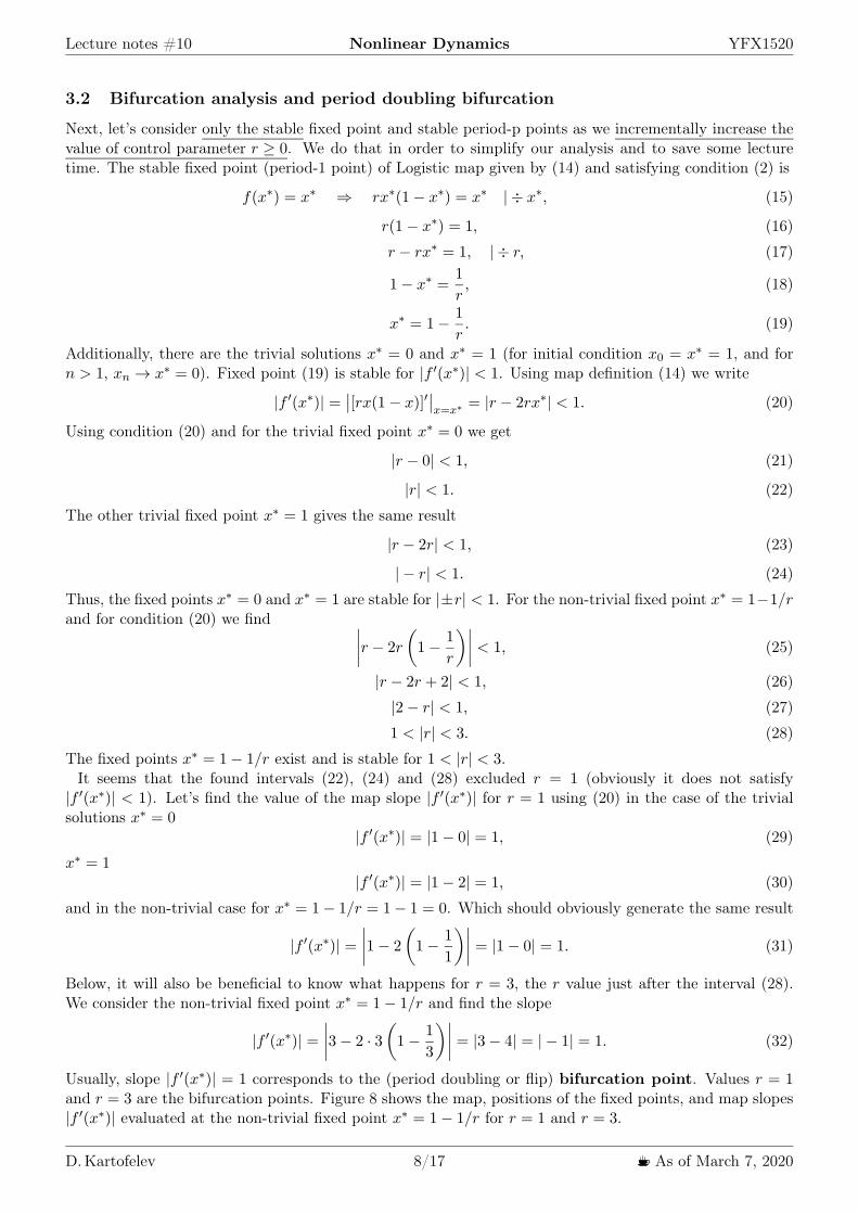
Lecture notes 10 Nonlinear Dynamics YFX1520
32 Bifurcation analysis and period doubling bifurcation
Next letrsquos consider only the stable fixed point and stable period-p points as we incrementally increase thevalue of control parameter r ge 0 We do that in order to simplify our analysis and to save some lecturetime The stable fixed point (period-1 point) of Logistic map given by (14) and satisfying condition (2) is
f(xlowast) = xlowast rArr rxlowast(1minus xlowast) = xlowast | divide xlowast (15)
r(1minus xlowast) = 1 (16)
r minus rxlowast = 1 | divide r (17)
1minus xlowast =1
r (18)
xlowast = 1minus 1
r (19)
Additionally there are the trivial solutions xlowast = 0 and xlowast = 1 (for initial condition x0 = xlowast = 1 and forn gt 1 xn rarr xlowast = 0) Fixed point (19) is stable for |f prime(xlowast)| lt 1 Using map definition (14) we write
|f prime(xlowast)| =983055983055[rx(1minus x)]prime
983055983055x=xlowast = |r minus 2rxlowast| lt 1 (20)
Using condition (20) and for the trivial fixed point xlowast = 0 we get
|r minus 0| lt 1 (21)
|r| lt 1 (22)
The other trivial fixed point xlowast = 1 gives the same result
|r minus 2r| lt 1 (23)
|minus r| lt 1 (24)
Thus the fixed points xlowast = 0 and xlowast = 1 are stable for |plusmnr| lt 1 For the non-trivial fixed point xlowast = 1minus1rand for condition (20) we find 983055983055983055983055r minus 2r
9830611minus 1
r
983062983055983055983055983055 lt 1 (25)
|r minus 2r + 2| lt 1 (26)
|2minus r| lt 1 (27)
1 lt |r| lt 3 (28)
The fixed points xlowast = 1minus 1r exist and is stable for 1 lt |r| lt 3It seems that the found intervals (22) (24) and (28) excluded r = 1 (obviously it does not satisfy
|f prime(xlowast)| lt 1) Letrsquos find the value of the map slope |f prime(xlowast)| for r = 1 using (20) in the case of the trivialsolutions xlowast = 0
|f prime(xlowast)| = |1minus 0| = 1 (29)
xlowast = 1|f prime(xlowast)| = |1minus 2| = 1 (30)
and in the non-trivial case for xlowast = 1minus 1r = 1minus 1 = 0 Which should obviously generate the same result
|f prime(xlowast)| =9830559830559830559830551minus 2
9830611minus 1
1
983062983055983055983055983055 = |1minus 0| = 1 (31)
Below it will also be beneficial to know what happens for r = 3 the r value just after the interval (28)We consider the non-trivial fixed point xlowast = 1minus 1r and find the slope
|f prime(xlowast)| =9830559830559830559830553minus 2 middot 3
9830611minus 1
3
983062983055983055983055983055 = |3minus 4| = |minus 1| = 1 (32)
Usually slope |f prime(xlowast)| = 1 corresponds to the (period doubling or flip) bifurcation point Values r = 1and r = 3 are the bifurcation points Figure 8 shows the map positions of the fixed points and map slopes|f prime(xlowast)| evaluated at the non-trivial fixed point xlowast = 1minus 1r for r = 1 and r = 3
D Kartofelev 817 1003211 As of March 7 2020
Lecture notes 10 Nonlinear Dynamics YFX1520
Figure 8 (Left) Map slope at the fixed points xlowast = 1 minus 1r (same as the trivial case xlowast = 0) for r = 1(Right) Map slope at the fixed points xlowast = 1minus 1r for r = 3
The following interactive numerical file show the dynamics of Logistic map for 0 le |r| lt 1 and 1 lt |r| lt 3
Numerics cdf2 nb2Cobweb diagram of the Logistic map Orbit diagram of the Logistic map Period doubling and orbitdiagram
00 02 04 06 08 1000
02
04
06
08
10
xn
xn+1
0 5 10 15 2000
02
04
06
08
10
n
xn
00 02 04 06 08 1000
02
04
06
08
10
xn
xn+1
0 5 10 15 2000
02
04
06
08
10
n
xn
Figure 9 (Top-left) Cobweb diagram of the Logistic map shown for r = 098 lt 1 The fixed pointxlowast = 0 (Top-right) Map iterates corresponding to the cobweb diagram shown on the left (Bottom-left)Cobweb diagram of the Logistic map shown for interval 1 lt |r| lt 3 with r = 282 The fixed pointxlowast = 1minus 1r (Bottom-right) Map iterates corresponding to the cobweb diagram shown on the left
What happens for r ge 3 What happens after the period doubling or flip bifurcation at r = 3 Thename ldquofliprdquo refers to the fact that the map trajectories start to flip between two values mdash period-2 pointsin period-2 orbit Letrsquos check the dynamics using a computer
Numerics cdf2 nb2Cobweb diagram of the Logistic map Orbit diagram of the Logistic map Period doubling and orbitdiagramAfter the initial transient behaviour has decayed the dynamics of the map settles to a stableperiod-2 orbit It can be showed that period-2 orbits exist for 3 le r lt 1 +
radic6
D Kartofelev 917 1003211 As of March 7 2020
Lecture notes 10 Nonlinear Dynamics YFX1520
00 02 04 06 08 1000
02
04
06
08
10
xn
xn+1
0 5 10 15 20 25 3000
02
04
06
08
10
n
xn
Figure 10 (Left) Cobweb diagram of the Logistic map shown for r = 319 ge 3 featuring the stableperiod-2 point (Right) Map iterates corresponding to the cobweb diagram shown on the left
Letrsquos try to think about this outcome some more
Slides 7ndash9
Logistic map period-2 window
Period-2 window for 3 r lt 1 +p6
Figure Logistic map where r = 318 and x0 = 035 Fixed points (fps)in the case where r lt 3 are shown with the grey bullets Period-2 pointsof f(x) map for r 3 are shown with the blue bullets The fixed points off2(x) map for r 3 are shown with the red bullets
DKartofelev YFX1520 7 18
Logistic map period-2 window
Period-2 window for 3 r lt 1 +p6
(f(p) = rp(1 p) = q
f(q) = rq(1 q) = p(10)
where period-2 point values p and q are the fps of f(x) map
On the other hand it also holds(f(p) = f(f(q)) f 2(q) = r[rq(1 q)][1 (rq(1 q))] = q
f(q) = f(f(p)) f 2(p) = r[rp(1 p)][1 (rp(1 p))] = p)
(11)) f 2(x) = r[rx(1 x)][1 (rx(1 x))] = x (12)
where period-2 point values p and q are the fps of f 2(x) map
DKartofelev YFX1520 8 18
If you want to study the dynamics of the attractors of second iterate map f2 analytically consider oneof the equations in (11 slide numbering) The fourth order polynomial defined by Eq (7)
r[rx(1minus x)][1minus (rx(1minus x))] = x (33)
minus r3x4 + 2r3x3 minus r2(1 + r)x2 + r2x = x (34)
Intersections between the graph of second iterate map f2 and the diagonal correspond to the solutionsof f2(x) = x (34)
Stability of fps of f 2map in period-2 orbit
We need to know the slopes of period-2 points(f(p) = rp(1 p) = q
f(q) = rq(1 q) = p
According to the chain rule it holds that
(f 2(x))0 (f(f(x))0 = f 0(f(x)) middot f 0(x) (13)
In our case
(f 2(p))0 = f 0(f(p)) middot f 0(p) = f 0(q) middot f 0(p)
(f 2(q))0 = f 0(f(q)) middot f 0(q) = f 0(p) middot f 0(q)
)) (f 2(p))0 = (f 2(q))0
(14)Above follows from the commutative property of multiplication
DKartofelev YFX1520 9 18
D Kartofelev 1017 1003211 As of March 7 2020
Lecture notes 10 Nonlinear Dynamics YFX1520
The slopes of map f2 at its fixed points p and q are equal and they are the products of map f slopesat its respective period-2 points
What happens for r ge 1 +radic6 Once again we use a computer
Numerics cdf2 nb2Cobweb diagram of the Logistic map Orbit diagram of the Logistic map Period doubling and orbitdiagram
A period-4 orbit has emerged It can be shown that period-4 orbits exist for 1 +radic6 le r lt 354409
00 02 04 06 08 1000
02
04
06
08
10
xn
xn+1
0 5 10 15 20 25 3000
02
04
06
08
10
n
xn
Figure 11 (Left) Cobweb diagram of the Logistic map shown for r = 3535 ge 1 +radic6 featuring the
stable period-4 point The blue graph shows fourth iterate map f4 (Right) Map iterates correspondingto the cobweb diagram of map f shown on the left
Figure 12 counts the period-4 pointsiterates in the period-4 orbit of the Logistic map Compare Fig 12 toFig 5
Figure 12 Period-4 orbit in the Logistic map
What have we seen so far As we have incrementally increased the value of control parameter r theperiods of the fixed points have increased as well mdash from period-1 to period-2 and finally to period-4The period is clearly doubling This type of bifurcation is called the period doubling bifurca-tion Further period-doublings to orbits of period-8 -16 -32 etc occur as r increases Specifically letrn denote the value of r where a stable 2n-orbit first appears Then computer experiments reveal that
D Kartofelev 1117 1003211 As of March 7 2020
Lecture notes 10 Nonlinear Dynamics YFX1520
Slide 10
Logistic map period doubling
Even number periods
rn ndash bifurcation point onset of stable period-2n orbit
r1 = 30 period-2r2 = 1 +
p6 344949 period-4
r3 354409 period-8r4 356441 period-16r5 356875 period-32r6 356969 period-64
r1 3569946 period-21
r1 ndash onset of chaos (the accumulation point)
= limn1
rn1 rn2
rn rn1 4669201609 (15)
DKartofelev YFX1520 10 18
Note that the successive bifurcations come faster and faster Ultimately the rn converge toa limiting value rinfin The convergence is (essentially) geometric (itrsquos geometric near rinfin) in the limitof large n the distance between successive transitions shrinks by a constant factor of δ This ratio iscalled the Feigenbaum constant After the accumulation point r gt rinfin the dynamics becomeschaotic as wersquoll see below
33 Orbit diagram
The orbit diagram is also called the fig tree diagram (Feigenbaum in German means ldquofig treerdquo) or (in-correctly) the Feigenbaum diagram You might guess that the system would become more and morechaotic for r gt rinfin as r increases but in fact the dynamics are more subtle than that To see the long-termbehaviour for all values of r at once we plot the orbit diagram a special kind of bifurcation diagramOrbit diagram plots the systemrsquos attractor (stable fixed points and stable period-p points) as a function ofcontrol parameter r
To generate the orbit diagram for yourself yoursquoll need to write a computer program with two loops Firstchoose a value of r Then generate an orbit starting from some random initial condition x0 Iterate for 300cycles or so to allow the system to settle down to its eventual stable behaviour Once the transients havedecayed plot many points say x301 x900 above that r Then move to an adjacent value of r and repeateventually sweeping across the whole diagram
The following interactive numerical file shows the orbit diagram for the Logistic map
Numerics cdf2 nb2Cobweb diagram of the Logistic map Orbit diagram of the Logistic map Period doubling and orbitdiagram
The connection between the cobweb diagram orbit diagram and the Lyapunov exponent is shown in theinteractive numerical file linked below
Numerics cdf3 nb3Logistic map cobweb diagram orbit diagram and map iterates Lyapunov exponent
D Kartofelev 1217 1003211 As of March 7 2020
Lecture notes 10 Nonlinear Dynamics YFX1520
Slides 11 12
Orbit diagram and period doubling
DKartofelev YFX1520 11 18
Zooming into the Logistic map self-similarity
No embedded video files in this pdf
DKartofelev YFX1520 12 18
The period doubling is driven by the subsequent flip bifurcations or supercritical pitchforkbifurcations (if we use the nomenclature introduced in Lecture 2) The unstable fixed point andperiod-p points are omitted from the orbit diagram
Feigenbaum diagram shows both stable and unstable fixed points and period-p points or simplydiagram branches (not shown here)
The orbit diagram of the Logistic map features self-similarity In mathematics a self-similarobject is (exactly or) approximately similar to a part of itself ie the whole has the same shape orquality as one or more of its sub-parts
34 Tangent bifurcation and odd number period-p points
Can an odd number period appear in the Logistic map mdash eg period-3 point One of the most intriguingfeatures of the orbit diagram is the occurrence of periodic windows for r gt rinfin The period-3 windowthat occurs for 1 +
radic8 le r le 38415 is the most conspicuous Suddenly against a backdrop of chaos a
stable period-3 orbit appears out of the blueLetrsquos see if we can find the period-3 window of Logistic map using a computer
Numerics cdf2 nb2Cobweb diagram of the Logistic map Orbit diagram of the Logistic map Period doubling and orbitdiagram
The tangent bifurcation is a new type of bifurcation for us that occurs at r = 1 +radic8
00 02 04 06 08 1000
02
04
06
08
10
xn
xn+1
0 5 10 15 20 25 3000
02
04
06
08
10
n
xn
Figure 13 (Left) Period-3 orbit of map f can be found in the period-3 window Here showing thetrajectory for r = 383 (Right) Map iterates corresponding to the cobweb diagram of map f shownon the left
The mechanism responsible for the occurrence of the odd number periods-p points is shown in Fig 14The intersections between the graph of f3 shown in red and the diagonal correspond to solutions of
D Kartofelev 1317 1003211 As of March 7 2020
Lecture notes 10 Nonlinear Dynamics YFX1520
Figure 14 Period-3 orbit can be found in period-3 window of the orbit diagram
f3(x) = x There are eight solutions for r ge 1+radic8 six of interest to us are marked with the blue dots and
two imposters that are not genuine period-3 they are actually fixed points or period-1 points for whichf(xlowast) = xlowast The blue filled dots in Fig 14 correspond to a stable period-3 cycle note that the slope off3(x) is shallow at these points consistent with the stability of the cycle In contrast the slope exceeds 1at the cycle marked by the empty blue dots this period-3 orbit is therefore unstable
Now suppose we decrease r toward the chaotic regime r lt 1+radic8 Then the red graph in Fig 14 changes
shape mdash the hill moves down and the valleys rise up The curve therefore moves towards the diagonalFigure 14 shows that when r = 1 +
radic8 the six blue intersections have merged to form three black filled
period-3 points by becoming tangent to the diagonal At this critical value of r the stable and unstableperiod-3 cycles coalesce and annihilate in a tangent bifurcation This transition defines the beginning ofthe periodic period-3 window
All odd number periods will also undergo the period doubling This means that all number periods [1infin)are eventually represented in the orbit diagram
Figure 14 also explains the self-similarity present in the orbit diagram as shown on Slide 12 for differentscales of magnification The peaks and valley of map f3 are smaller distorted copies of the original mapf Thus the local dynamics of the cobweb trajectories for map f3 must be similar to the dynamics of theoriginal map f
Slide 13
Intermittency3and period-3 window
Transient chaos and intermittency in dynamical systemsTangent bifurcation occurs at r = 1 +
p8 38284 (period-3 orbit)
50 100 150n
02
04
06
08
10xn
Iterates of Logistic map shown for r = 38282 and x0 = 015
3See Mathematica nb file uploaded to course webpageDKartofelev YFX1520 13 18
The dynamics closely related to the tangent bifurcation is intermittency Logistic map exhibitsintermittent chaos for r values just before the period-3 window
D Kartofelev 1417 1003211 As of March 7 2020
Lecture notes 10 Nonlinear Dynamics YFX1520
Numerics cdf4 nb4Period-3 window and intermittency in the Logistic map (iterates xn)
4 Sine map and universality of period doubling
It can be shown that in all unimodal maps same dynamics of period doubling occurs For example weconsider the sine map
Slide 14
Universality of period doubling in unimodal maps
1-D sine map4 The sine map has the form
xn+1 = r sin(xn) x0 2 [0 1] r 2 [0 1] n 2 Z+ (16)
where r is the control parameter
Read Mitchell J Feigenbaum ldquoQuantitative universality for a classof nonlinear transformationsrdquo Journal of Statistical Physics 19(1)pp 25ndash52 1978 doi101007BF01020332
Read Mitchell J Feigenbaum ldquoUniversal behavior in nonlinearsystemsrdquo Physica D Nonlinear Phenomena 7(1ndash3) pp 16ndash391983 doi1010160167-2789(83)90112-4
4See Mathematica nb file (cobweb diagram and orbit diagram) uploaded tothe course webpage
DKartofelev YFX1520 14 18
The graph of the sine map has the same basic shape as the graph of the Logistic map Both curvesare smooth concave down and have a single maximum Such maps are called unimodal
Sine is also a transcendental function opposed to an algebraic function as is the polynomial thatdescribes the Logistic map A transcendental function is an analytic function that does not satisfy apolynomial equation In other words a transcendental function ldquotranscendsrdquo algebra in that it cannotbe expressed in terms of a finite sequence of the algebraic operations of addition multiplication androot extraction
The transcendental nature of the sine map must makes the underlying higher-dimensional physicsrepresented by the sine map fundamentally different from eg the three-dimensional Lorenz flowsampled by Lorenz map
Letrsquos study the dynamics of the sine map using a computer
Numerics cdf5 nb5The sine map iterates cobweb and orbit diagrams (xn isin [0 1])
Numerics cdf6 nb6The sine map iterates cobweb and orbit diagrams (xn isin [minus1 1])
The dynamics is surprisingly similar to the dynamics of the Logistic map Mitchell J Feigenbaumwas first to discover the quantitative laws that are independent of unimodal map functions f Bythat we mean that the algebraic form of f(x) is irrelevant only its overall shape matters
D Kartofelev 1517 1003211 As of March 7 2020
Lecture notes 10 Nonlinear Dynamics YFX1520
Slide 151-D unimodal maps and Feigenbaum constants
= limn1
n1
n= lim
n1
rn1 rn2
rn rn1 4669201609 (17)
crarr = limn1
dn1
dn 2502907875 (18)
DKartofelev YFX1520 15 18
Here xm = max f(x) is the maximum of the map graph The Feigenbaum constants are valid up tothe onset of chaos at rinfin and inside each periodic window for r gt rinfin
In addition to scaling law in control parameter r direction shown earlier Feigenbaum also foundscaling law for the vertical x-direction of the orbit diagram The Feigenbaum constants are uni-versal the same convergence rate appears no matter what unimodal map is iterated They are newmathematical constants as basic to period doubling as π is to circles
Reading suggestion
Link File name CitationPaper2 paper3pdf Mitchell J Feigenbaum ldquoQuantitative universality for a class of nonlinear trans-
formationsrdquo Journal of Statistical Physics 19(1) pp 25ndash52 (1978)doi101007BF01020332
Paper3 paper4pdf Mitchell J Feigenbaum ldquoUniversal behavior in nonlinear systemsrdquo Physica DNonlinear Phenomena 7(1ndash3) pp 16ndash39 (1983)doi1010160167-2789(83)90112-4
5 Universal route to chaos
We showed that the qualitative dynamics of the Logistic and sine maps are identical They both undergoperiod doubling routes to chaos followed by periodic windows interwoven with chaotic bandsEven more remarkably the periodic windows occur in the same order and with the same relative sizes Forinstance the period-3 window is the largest in both cases and the next largest windows preceding it areperiod-5 and period-6 But there are quantitative differences For instance the period doubling bifurcationsoccur later (for greater parameter r value) in the Logistic map and the periodic windows are thinner
Turns out that the onset of chaos via period doubling is predominant in nature and in artificial chaoticsystems Feigenbaum constants have real predictive power in various scientific applications The perioddoubling bifurcation is the ldquorouterdquo taken by nonlinear systems to reach chaotic solution Interm of the bifurcations introduced in Lecture 2 the period doubling bifurcation can also be seen as a seriesof subsequentsucceeding supercritical pitchfork bifurcations see Slide 11
Revision questions
1 What is cobweb diagram2 What is recurrence map or recurrence relation3 What is 1-D map4 How to find fixed points of 1-D maps5 What is Lorenz map
D Kartofelev 1617 1003211 As of March 7 2020
Lecture notes 10 Nonlinear Dynamics YFX1520
6 What is Logistic map7 What is sine map8 What is period doubling9 What is period doubling bifurcation
10 What is tangent bifurcation11 Do odd number periods (period-p orbits) exist in chaotic systems12 Do even number periods (period-p orbits) exist in chaotic systems13 Can maps produce transient chaos14 Can maps produce intermittency15 Can maps produce intermittent chaos16 What is orbit diagram (or Feigenbaum diagram)17 What are Feigenbaum constants
D Kartofelev 1717 1003211 As of March 7 2020
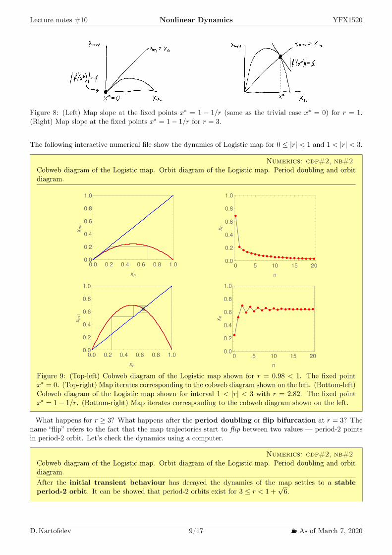
Lecture notes 10 Nonlinear Dynamics YFX1520
Figure 8 (Left) Map slope at the fixed points xlowast = 1 minus 1r (same as the trivial case xlowast = 0) for r = 1(Right) Map slope at the fixed points xlowast = 1minus 1r for r = 3
The following interactive numerical file show the dynamics of Logistic map for 0 le |r| lt 1 and 1 lt |r| lt 3
Numerics cdf2 nb2Cobweb diagram of the Logistic map Orbit diagram of the Logistic map Period doubling and orbitdiagram
00 02 04 06 08 1000
02
04
06
08
10
xn
xn+1
0 5 10 15 2000
02
04
06
08
10
n
xn
00 02 04 06 08 1000
02
04
06
08
10
xn
xn+1
0 5 10 15 2000
02
04
06
08
10
n
xn
Figure 9 (Top-left) Cobweb diagram of the Logistic map shown for r = 098 lt 1 The fixed pointxlowast = 0 (Top-right) Map iterates corresponding to the cobweb diagram shown on the left (Bottom-left)Cobweb diagram of the Logistic map shown for interval 1 lt |r| lt 3 with r = 282 The fixed pointxlowast = 1minus 1r (Bottom-right) Map iterates corresponding to the cobweb diagram shown on the left
What happens for r ge 3 What happens after the period doubling or flip bifurcation at r = 3 Thename ldquofliprdquo refers to the fact that the map trajectories start to flip between two values mdash period-2 pointsin period-2 orbit Letrsquos check the dynamics using a computer
Numerics cdf2 nb2Cobweb diagram of the Logistic map Orbit diagram of the Logistic map Period doubling and orbitdiagramAfter the initial transient behaviour has decayed the dynamics of the map settles to a stableperiod-2 orbit It can be showed that period-2 orbits exist for 3 le r lt 1 +
radic6
D Kartofelev 917 1003211 As of March 7 2020
Lecture notes 10 Nonlinear Dynamics YFX1520
00 02 04 06 08 1000
02
04
06
08
10
xn
xn+1
0 5 10 15 20 25 3000
02
04
06
08
10
n
xn
Figure 10 (Left) Cobweb diagram of the Logistic map shown for r = 319 ge 3 featuring the stableperiod-2 point (Right) Map iterates corresponding to the cobweb diagram shown on the left
Letrsquos try to think about this outcome some more
Slides 7ndash9
Logistic map period-2 window
Period-2 window for 3 r lt 1 +p6
Figure Logistic map where r = 318 and x0 = 035 Fixed points (fps)in the case where r lt 3 are shown with the grey bullets Period-2 pointsof f(x) map for r 3 are shown with the blue bullets The fixed points off2(x) map for r 3 are shown with the red bullets
DKartofelev YFX1520 7 18
Logistic map period-2 window
Period-2 window for 3 r lt 1 +p6
(f(p) = rp(1 p) = q
f(q) = rq(1 q) = p(10)
where period-2 point values p and q are the fps of f(x) map
On the other hand it also holds(f(p) = f(f(q)) f 2(q) = r[rq(1 q)][1 (rq(1 q))] = q
f(q) = f(f(p)) f 2(p) = r[rp(1 p)][1 (rp(1 p))] = p)
(11)) f 2(x) = r[rx(1 x)][1 (rx(1 x))] = x (12)
where period-2 point values p and q are the fps of f 2(x) map
DKartofelev YFX1520 8 18
If you want to study the dynamics of the attractors of second iterate map f2 analytically consider oneof the equations in (11 slide numbering) The fourth order polynomial defined by Eq (7)
r[rx(1minus x)][1minus (rx(1minus x))] = x (33)
minus r3x4 + 2r3x3 minus r2(1 + r)x2 + r2x = x (34)
Intersections between the graph of second iterate map f2 and the diagonal correspond to the solutionsof f2(x) = x (34)
Stability of fps of f 2map in period-2 orbit
We need to know the slopes of period-2 points(f(p) = rp(1 p) = q
f(q) = rq(1 q) = p
According to the chain rule it holds that
(f 2(x))0 (f(f(x))0 = f 0(f(x)) middot f 0(x) (13)
In our case
(f 2(p))0 = f 0(f(p)) middot f 0(p) = f 0(q) middot f 0(p)
(f 2(q))0 = f 0(f(q)) middot f 0(q) = f 0(p) middot f 0(q)
)) (f 2(p))0 = (f 2(q))0
(14)Above follows from the commutative property of multiplication
DKartofelev YFX1520 9 18
D Kartofelev 1017 1003211 As of March 7 2020
Lecture notes 10 Nonlinear Dynamics YFX1520
The slopes of map f2 at its fixed points p and q are equal and they are the products of map f slopesat its respective period-2 points
What happens for r ge 1 +radic6 Once again we use a computer
Numerics cdf2 nb2Cobweb diagram of the Logistic map Orbit diagram of the Logistic map Period doubling and orbitdiagram
A period-4 orbit has emerged It can be shown that period-4 orbits exist for 1 +radic6 le r lt 354409
00 02 04 06 08 1000
02
04
06
08
10
xn
xn+1
0 5 10 15 20 25 3000
02
04
06
08
10
n
xn
Figure 11 (Left) Cobweb diagram of the Logistic map shown for r = 3535 ge 1 +radic6 featuring the
stable period-4 point The blue graph shows fourth iterate map f4 (Right) Map iterates correspondingto the cobweb diagram of map f shown on the left
Figure 12 counts the period-4 pointsiterates in the period-4 orbit of the Logistic map Compare Fig 12 toFig 5
Figure 12 Period-4 orbit in the Logistic map
What have we seen so far As we have incrementally increased the value of control parameter r theperiods of the fixed points have increased as well mdash from period-1 to period-2 and finally to period-4The period is clearly doubling This type of bifurcation is called the period doubling bifurca-tion Further period-doublings to orbits of period-8 -16 -32 etc occur as r increases Specifically letrn denote the value of r where a stable 2n-orbit first appears Then computer experiments reveal that
D Kartofelev 1117 1003211 As of March 7 2020
Lecture notes 10 Nonlinear Dynamics YFX1520
Slide 10
Logistic map period doubling
Even number periods
rn ndash bifurcation point onset of stable period-2n orbit
r1 = 30 period-2r2 = 1 +
p6 344949 period-4
r3 354409 period-8r4 356441 period-16r5 356875 period-32r6 356969 period-64
r1 3569946 period-21
r1 ndash onset of chaos (the accumulation point)
= limn1
rn1 rn2
rn rn1 4669201609 (15)
DKartofelev YFX1520 10 18
Note that the successive bifurcations come faster and faster Ultimately the rn converge toa limiting value rinfin The convergence is (essentially) geometric (itrsquos geometric near rinfin) in the limitof large n the distance between successive transitions shrinks by a constant factor of δ This ratio iscalled the Feigenbaum constant After the accumulation point r gt rinfin the dynamics becomeschaotic as wersquoll see below
33 Orbit diagram
The orbit diagram is also called the fig tree diagram (Feigenbaum in German means ldquofig treerdquo) or (in-correctly) the Feigenbaum diagram You might guess that the system would become more and morechaotic for r gt rinfin as r increases but in fact the dynamics are more subtle than that To see the long-termbehaviour for all values of r at once we plot the orbit diagram a special kind of bifurcation diagramOrbit diagram plots the systemrsquos attractor (stable fixed points and stable period-p points) as a function ofcontrol parameter r
To generate the orbit diagram for yourself yoursquoll need to write a computer program with two loops Firstchoose a value of r Then generate an orbit starting from some random initial condition x0 Iterate for 300cycles or so to allow the system to settle down to its eventual stable behaviour Once the transients havedecayed plot many points say x301 x900 above that r Then move to an adjacent value of r and repeateventually sweeping across the whole diagram
The following interactive numerical file shows the orbit diagram for the Logistic map
Numerics cdf2 nb2Cobweb diagram of the Logistic map Orbit diagram of the Logistic map Period doubling and orbitdiagram
The connection between the cobweb diagram orbit diagram and the Lyapunov exponent is shown in theinteractive numerical file linked below
Numerics cdf3 nb3Logistic map cobweb diagram orbit diagram and map iterates Lyapunov exponent
D Kartofelev 1217 1003211 As of March 7 2020
Lecture notes 10 Nonlinear Dynamics YFX1520
Slides 11 12
Orbit diagram and period doubling
DKartofelev YFX1520 11 18
Zooming into the Logistic map self-similarity
No embedded video files in this pdf
DKartofelev YFX1520 12 18
The period doubling is driven by the subsequent flip bifurcations or supercritical pitchforkbifurcations (if we use the nomenclature introduced in Lecture 2) The unstable fixed point andperiod-p points are omitted from the orbit diagram
Feigenbaum diagram shows both stable and unstable fixed points and period-p points or simplydiagram branches (not shown here)
The orbit diagram of the Logistic map features self-similarity In mathematics a self-similarobject is (exactly or) approximately similar to a part of itself ie the whole has the same shape orquality as one or more of its sub-parts
34 Tangent bifurcation and odd number period-p points
Can an odd number period appear in the Logistic map mdash eg period-3 point One of the most intriguingfeatures of the orbit diagram is the occurrence of periodic windows for r gt rinfin The period-3 windowthat occurs for 1 +
radic8 le r le 38415 is the most conspicuous Suddenly against a backdrop of chaos a
stable period-3 orbit appears out of the blueLetrsquos see if we can find the period-3 window of Logistic map using a computer
Numerics cdf2 nb2Cobweb diagram of the Logistic map Orbit diagram of the Logistic map Period doubling and orbitdiagram
The tangent bifurcation is a new type of bifurcation for us that occurs at r = 1 +radic8
00 02 04 06 08 1000
02
04
06
08
10
xn
xn+1
0 5 10 15 20 25 3000
02
04
06
08
10
n
xn
Figure 13 (Left) Period-3 orbit of map f can be found in the period-3 window Here showing thetrajectory for r = 383 (Right) Map iterates corresponding to the cobweb diagram of map f shownon the left
The mechanism responsible for the occurrence of the odd number periods-p points is shown in Fig 14The intersections between the graph of f3 shown in red and the diagonal correspond to solutions of
D Kartofelev 1317 1003211 As of March 7 2020
Lecture notes 10 Nonlinear Dynamics YFX1520
Figure 14 Period-3 orbit can be found in period-3 window of the orbit diagram
f3(x) = x There are eight solutions for r ge 1+radic8 six of interest to us are marked with the blue dots and
two imposters that are not genuine period-3 they are actually fixed points or period-1 points for whichf(xlowast) = xlowast The blue filled dots in Fig 14 correspond to a stable period-3 cycle note that the slope off3(x) is shallow at these points consistent with the stability of the cycle In contrast the slope exceeds 1at the cycle marked by the empty blue dots this period-3 orbit is therefore unstable
Now suppose we decrease r toward the chaotic regime r lt 1+radic8 Then the red graph in Fig 14 changes
shape mdash the hill moves down and the valleys rise up The curve therefore moves towards the diagonalFigure 14 shows that when r = 1 +
radic8 the six blue intersections have merged to form three black filled
period-3 points by becoming tangent to the diagonal At this critical value of r the stable and unstableperiod-3 cycles coalesce and annihilate in a tangent bifurcation This transition defines the beginning ofthe periodic period-3 window
All odd number periods will also undergo the period doubling This means that all number periods [1infin)are eventually represented in the orbit diagram
Figure 14 also explains the self-similarity present in the orbit diagram as shown on Slide 12 for differentscales of magnification The peaks and valley of map f3 are smaller distorted copies of the original mapf Thus the local dynamics of the cobweb trajectories for map f3 must be similar to the dynamics of theoriginal map f
Slide 13
Intermittency3and period-3 window
Transient chaos and intermittency in dynamical systemsTangent bifurcation occurs at r = 1 +
p8 38284 (period-3 orbit)
50 100 150n
02
04
06
08
10xn
Iterates of Logistic map shown for r = 38282 and x0 = 015
3See Mathematica nb file uploaded to course webpageDKartofelev YFX1520 13 18
The dynamics closely related to the tangent bifurcation is intermittency Logistic map exhibitsintermittent chaos for r values just before the period-3 window
D Kartofelev 1417 1003211 As of March 7 2020
Lecture notes 10 Nonlinear Dynamics YFX1520
Numerics cdf4 nb4Period-3 window and intermittency in the Logistic map (iterates xn)
4 Sine map and universality of period doubling
It can be shown that in all unimodal maps same dynamics of period doubling occurs For example weconsider the sine map
Slide 14
Universality of period doubling in unimodal maps
1-D sine map4 The sine map has the form
xn+1 = r sin(xn) x0 2 [0 1] r 2 [0 1] n 2 Z+ (16)
where r is the control parameter
Read Mitchell J Feigenbaum ldquoQuantitative universality for a classof nonlinear transformationsrdquo Journal of Statistical Physics 19(1)pp 25ndash52 1978 doi101007BF01020332
Read Mitchell J Feigenbaum ldquoUniversal behavior in nonlinearsystemsrdquo Physica D Nonlinear Phenomena 7(1ndash3) pp 16ndash391983 doi1010160167-2789(83)90112-4
4See Mathematica nb file (cobweb diagram and orbit diagram) uploaded tothe course webpage
DKartofelev YFX1520 14 18
The graph of the sine map has the same basic shape as the graph of the Logistic map Both curvesare smooth concave down and have a single maximum Such maps are called unimodal
Sine is also a transcendental function opposed to an algebraic function as is the polynomial thatdescribes the Logistic map A transcendental function is an analytic function that does not satisfy apolynomial equation In other words a transcendental function ldquotranscendsrdquo algebra in that it cannotbe expressed in terms of a finite sequence of the algebraic operations of addition multiplication androot extraction
The transcendental nature of the sine map must makes the underlying higher-dimensional physicsrepresented by the sine map fundamentally different from eg the three-dimensional Lorenz flowsampled by Lorenz map
Letrsquos study the dynamics of the sine map using a computer
Numerics cdf5 nb5The sine map iterates cobweb and orbit diagrams (xn isin [0 1])
Numerics cdf6 nb6The sine map iterates cobweb and orbit diagrams (xn isin [minus1 1])
The dynamics is surprisingly similar to the dynamics of the Logistic map Mitchell J Feigenbaumwas first to discover the quantitative laws that are independent of unimodal map functions f Bythat we mean that the algebraic form of f(x) is irrelevant only its overall shape matters
D Kartofelev 1517 1003211 As of March 7 2020
Lecture notes 10 Nonlinear Dynamics YFX1520
Slide 151-D unimodal maps and Feigenbaum constants
= limn1
n1
n= lim
n1
rn1 rn2
rn rn1 4669201609 (17)
crarr = limn1
dn1
dn 2502907875 (18)
DKartofelev YFX1520 15 18
Here xm = max f(x) is the maximum of the map graph The Feigenbaum constants are valid up tothe onset of chaos at rinfin and inside each periodic window for r gt rinfin
In addition to scaling law in control parameter r direction shown earlier Feigenbaum also foundscaling law for the vertical x-direction of the orbit diagram The Feigenbaum constants are uni-versal the same convergence rate appears no matter what unimodal map is iterated They are newmathematical constants as basic to period doubling as π is to circles
Reading suggestion
Link File name CitationPaper2 paper3pdf Mitchell J Feigenbaum ldquoQuantitative universality for a class of nonlinear trans-
formationsrdquo Journal of Statistical Physics 19(1) pp 25ndash52 (1978)doi101007BF01020332
Paper3 paper4pdf Mitchell J Feigenbaum ldquoUniversal behavior in nonlinear systemsrdquo Physica DNonlinear Phenomena 7(1ndash3) pp 16ndash39 (1983)doi1010160167-2789(83)90112-4
5 Universal route to chaos
We showed that the qualitative dynamics of the Logistic and sine maps are identical They both undergoperiod doubling routes to chaos followed by periodic windows interwoven with chaotic bandsEven more remarkably the periodic windows occur in the same order and with the same relative sizes Forinstance the period-3 window is the largest in both cases and the next largest windows preceding it areperiod-5 and period-6 But there are quantitative differences For instance the period doubling bifurcationsoccur later (for greater parameter r value) in the Logistic map and the periodic windows are thinner
Turns out that the onset of chaos via period doubling is predominant in nature and in artificial chaoticsystems Feigenbaum constants have real predictive power in various scientific applications The perioddoubling bifurcation is the ldquorouterdquo taken by nonlinear systems to reach chaotic solution Interm of the bifurcations introduced in Lecture 2 the period doubling bifurcation can also be seen as a seriesof subsequentsucceeding supercritical pitchfork bifurcations see Slide 11
Revision questions
1 What is cobweb diagram2 What is recurrence map or recurrence relation3 What is 1-D map4 How to find fixed points of 1-D maps5 What is Lorenz map
D Kartofelev 1617 1003211 As of March 7 2020
Lecture notes 10 Nonlinear Dynamics YFX1520
6 What is Logistic map7 What is sine map8 What is period doubling9 What is period doubling bifurcation
10 What is tangent bifurcation11 Do odd number periods (period-p orbits) exist in chaotic systems12 Do even number periods (period-p orbits) exist in chaotic systems13 Can maps produce transient chaos14 Can maps produce intermittency15 Can maps produce intermittent chaos16 What is orbit diagram (or Feigenbaum diagram)17 What are Feigenbaum constants
D Kartofelev 1717 1003211 As of March 7 2020
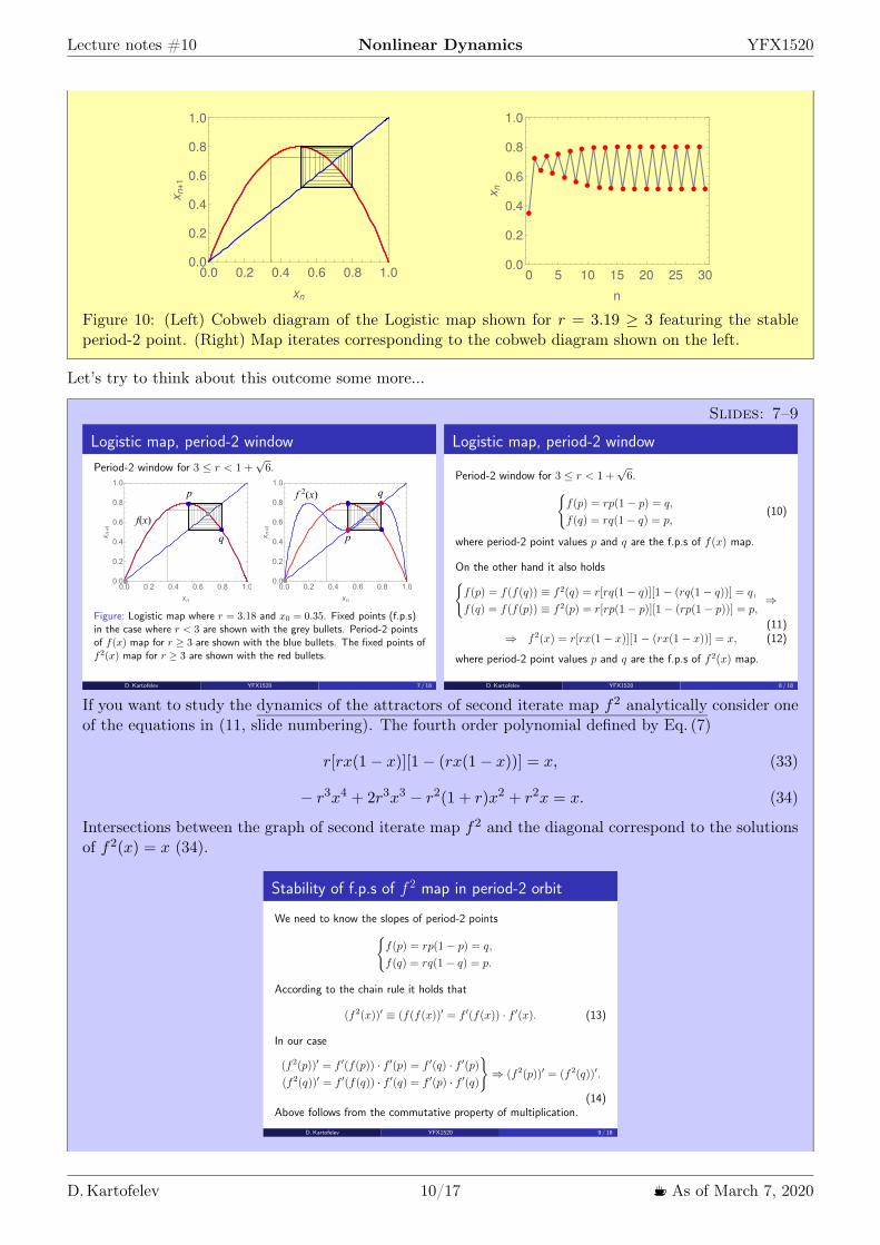
Lecture notes 10 Nonlinear Dynamics YFX1520
00 02 04 06 08 1000
02
04
06
08
10
xn
xn+1
0 5 10 15 20 25 3000
02
04
06
08
10
n
xn
Figure 10 (Left) Cobweb diagram of the Logistic map shown for r = 319 ge 3 featuring the stableperiod-2 point (Right) Map iterates corresponding to the cobweb diagram shown on the left
Letrsquos try to think about this outcome some more
Slides 7ndash9
Logistic map period-2 window
Period-2 window for 3 r lt 1 +p6
Figure Logistic map where r = 318 and x0 = 035 Fixed points (fps)in the case where r lt 3 are shown with the grey bullets Period-2 pointsof f(x) map for r 3 are shown with the blue bullets The fixed points off2(x) map for r 3 are shown with the red bullets
DKartofelev YFX1520 7 18
Logistic map period-2 window
Period-2 window for 3 r lt 1 +p6
(f(p) = rp(1 p) = q
f(q) = rq(1 q) = p(10)
where period-2 point values p and q are the fps of f(x) map
On the other hand it also holds(f(p) = f(f(q)) f 2(q) = r[rq(1 q)][1 (rq(1 q))] = q
f(q) = f(f(p)) f 2(p) = r[rp(1 p)][1 (rp(1 p))] = p)
(11)) f 2(x) = r[rx(1 x)][1 (rx(1 x))] = x (12)
where period-2 point values p and q are the fps of f 2(x) map
DKartofelev YFX1520 8 18
If you want to study the dynamics of the attractors of second iterate map f2 analytically consider oneof the equations in (11 slide numbering) The fourth order polynomial defined by Eq (7)
r[rx(1minus x)][1minus (rx(1minus x))] = x (33)
minus r3x4 + 2r3x3 minus r2(1 + r)x2 + r2x = x (34)
Intersections between the graph of second iterate map f2 and the diagonal correspond to the solutionsof f2(x) = x (34)
Stability of fps of f 2map in period-2 orbit
We need to know the slopes of period-2 points(f(p) = rp(1 p) = q
f(q) = rq(1 q) = p
According to the chain rule it holds that
(f 2(x))0 (f(f(x))0 = f 0(f(x)) middot f 0(x) (13)
In our case
(f 2(p))0 = f 0(f(p)) middot f 0(p) = f 0(q) middot f 0(p)
(f 2(q))0 = f 0(f(q)) middot f 0(q) = f 0(p) middot f 0(q)
)) (f 2(p))0 = (f 2(q))0
(14)Above follows from the commutative property of multiplication
DKartofelev YFX1520 9 18
D Kartofelev 1017 1003211 As of March 7 2020
Lecture notes 10 Nonlinear Dynamics YFX1520
The slopes of map f2 at its fixed points p and q are equal and they are the products of map f slopesat its respective period-2 points
What happens for r ge 1 +radic6 Once again we use a computer
Numerics cdf2 nb2Cobweb diagram of the Logistic map Orbit diagram of the Logistic map Period doubling and orbitdiagram
A period-4 orbit has emerged It can be shown that period-4 orbits exist for 1 +radic6 le r lt 354409
00 02 04 06 08 1000
02
04
06
08
10
xn
xn+1
0 5 10 15 20 25 3000
02
04
06
08
10
n
xn
Figure 11 (Left) Cobweb diagram of the Logistic map shown for r = 3535 ge 1 +radic6 featuring the
stable period-4 point The blue graph shows fourth iterate map f4 (Right) Map iterates correspondingto the cobweb diagram of map f shown on the left
Figure 12 counts the period-4 pointsiterates in the period-4 orbit of the Logistic map Compare Fig 12 toFig 5
Figure 12 Period-4 orbit in the Logistic map
What have we seen so far As we have incrementally increased the value of control parameter r theperiods of the fixed points have increased as well mdash from period-1 to period-2 and finally to period-4The period is clearly doubling This type of bifurcation is called the period doubling bifurca-tion Further period-doublings to orbits of period-8 -16 -32 etc occur as r increases Specifically letrn denote the value of r where a stable 2n-orbit first appears Then computer experiments reveal that
D Kartofelev 1117 1003211 As of March 7 2020
Lecture notes 10 Nonlinear Dynamics YFX1520
Slide 10
Logistic map period doubling
Even number periods
rn ndash bifurcation point onset of stable period-2n orbit
r1 = 30 period-2r2 = 1 +
p6 344949 period-4
r3 354409 period-8r4 356441 period-16r5 356875 period-32r6 356969 period-64
r1 3569946 period-21
r1 ndash onset of chaos (the accumulation point)
= limn1
rn1 rn2
rn rn1 4669201609 (15)
DKartofelev YFX1520 10 18
Note that the successive bifurcations come faster and faster Ultimately the rn converge toa limiting value rinfin The convergence is (essentially) geometric (itrsquos geometric near rinfin) in the limitof large n the distance between successive transitions shrinks by a constant factor of δ This ratio iscalled the Feigenbaum constant After the accumulation point r gt rinfin the dynamics becomeschaotic as wersquoll see below
33 Orbit diagram
The orbit diagram is also called the fig tree diagram (Feigenbaum in German means ldquofig treerdquo) or (in-correctly) the Feigenbaum diagram You might guess that the system would become more and morechaotic for r gt rinfin as r increases but in fact the dynamics are more subtle than that To see the long-termbehaviour for all values of r at once we plot the orbit diagram a special kind of bifurcation diagramOrbit diagram plots the systemrsquos attractor (stable fixed points and stable period-p points) as a function ofcontrol parameter r
To generate the orbit diagram for yourself yoursquoll need to write a computer program with two loops Firstchoose a value of r Then generate an orbit starting from some random initial condition x0 Iterate for 300cycles or so to allow the system to settle down to its eventual stable behaviour Once the transients havedecayed plot many points say x301 x900 above that r Then move to an adjacent value of r and repeateventually sweeping across the whole diagram
The following interactive numerical file shows the orbit diagram for the Logistic map
Numerics cdf2 nb2Cobweb diagram of the Logistic map Orbit diagram of the Logistic map Period doubling and orbitdiagram
The connection between the cobweb diagram orbit diagram and the Lyapunov exponent is shown in theinteractive numerical file linked below
Numerics cdf3 nb3Logistic map cobweb diagram orbit diagram and map iterates Lyapunov exponent
D Kartofelev 1217 1003211 As of March 7 2020
Lecture notes 10 Nonlinear Dynamics YFX1520
Slides 11 12
Orbit diagram and period doubling
DKartofelev YFX1520 11 18
Zooming into the Logistic map self-similarity
No embedded video files in this pdf
DKartofelev YFX1520 12 18
The period doubling is driven by the subsequent flip bifurcations or supercritical pitchforkbifurcations (if we use the nomenclature introduced in Lecture 2) The unstable fixed point andperiod-p points are omitted from the orbit diagram
Feigenbaum diagram shows both stable and unstable fixed points and period-p points or simplydiagram branches (not shown here)
The orbit diagram of the Logistic map features self-similarity In mathematics a self-similarobject is (exactly or) approximately similar to a part of itself ie the whole has the same shape orquality as one or more of its sub-parts
34 Tangent bifurcation and odd number period-p points
Can an odd number period appear in the Logistic map mdash eg period-3 point One of the most intriguingfeatures of the orbit diagram is the occurrence of periodic windows for r gt rinfin The period-3 windowthat occurs for 1 +
radic8 le r le 38415 is the most conspicuous Suddenly against a backdrop of chaos a
stable period-3 orbit appears out of the blueLetrsquos see if we can find the period-3 window of Logistic map using a computer
Numerics cdf2 nb2Cobweb diagram of the Logistic map Orbit diagram of the Logistic map Period doubling and orbitdiagram
The tangent bifurcation is a new type of bifurcation for us that occurs at r = 1 +radic8
00 02 04 06 08 1000
02
04
06
08
10
xn
xn+1
0 5 10 15 20 25 3000
02
04
06
08
10
n
xn
Figure 13 (Left) Period-3 orbit of map f can be found in the period-3 window Here showing thetrajectory for r = 383 (Right) Map iterates corresponding to the cobweb diagram of map f shownon the left
The mechanism responsible for the occurrence of the odd number periods-p points is shown in Fig 14The intersections between the graph of f3 shown in red and the diagonal correspond to solutions of
D Kartofelev 1317 1003211 As of March 7 2020
Lecture notes 10 Nonlinear Dynamics YFX1520
Figure 14 Period-3 orbit can be found in period-3 window of the orbit diagram
f3(x) = x There are eight solutions for r ge 1+radic8 six of interest to us are marked with the blue dots and
two imposters that are not genuine period-3 they are actually fixed points or period-1 points for whichf(xlowast) = xlowast The blue filled dots in Fig 14 correspond to a stable period-3 cycle note that the slope off3(x) is shallow at these points consistent with the stability of the cycle In contrast the slope exceeds 1at the cycle marked by the empty blue dots this period-3 orbit is therefore unstable
Now suppose we decrease r toward the chaotic regime r lt 1+radic8 Then the red graph in Fig 14 changes
shape mdash the hill moves down and the valleys rise up The curve therefore moves towards the diagonalFigure 14 shows that when r = 1 +
radic8 the six blue intersections have merged to form three black filled
period-3 points by becoming tangent to the diagonal At this critical value of r the stable and unstableperiod-3 cycles coalesce and annihilate in a tangent bifurcation This transition defines the beginning ofthe periodic period-3 window
All odd number periods will also undergo the period doubling This means that all number periods [1infin)are eventually represented in the orbit diagram
Figure 14 also explains the self-similarity present in the orbit diagram as shown on Slide 12 for differentscales of magnification The peaks and valley of map f3 are smaller distorted copies of the original mapf Thus the local dynamics of the cobweb trajectories for map f3 must be similar to the dynamics of theoriginal map f
Slide 13
Intermittency3and period-3 window
Transient chaos and intermittency in dynamical systemsTangent bifurcation occurs at r = 1 +
p8 38284 (period-3 orbit)
50 100 150n
02
04
06
08
10xn
Iterates of Logistic map shown for r = 38282 and x0 = 015
3See Mathematica nb file uploaded to course webpageDKartofelev YFX1520 13 18
The dynamics closely related to the tangent bifurcation is intermittency Logistic map exhibitsintermittent chaos for r values just before the period-3 window
D Kartofelev 1417 1003211 As of March 7 2020
Lecture notes 10 Nonlinear Dynamics YFX1520
Numerics cdf4 nb4Period-3 window and intermittency in the Logistic map (iterates xn)
4 Sine map and universality of period doubling
It can be shown that in all unimodal maps same dynamics of period doubling occurs For example weconsider the sine map
Slide 14
Universality of period doubling in unimodal maps
1-D sine map4 The sine map has the form
xn+1 = r sin(xn) x0 2 [0 1] r 2 [0 1] n 2 Z+ (16)
where r is the control parameter
Read Mitchell J Feigenbaum ldquoQuantitative universality for a classof nonlinear transformationsrdquo Journal of Statistical Physics 19(1)pp 25ndash52 1978 doi101007BF01020332
Read Mitchell J Feigenbaum ldquoUniversal behavior in nonlinearsystemsrdquo Physica D Nonlinear Phenomena 7(1ndash3) pp 16ndash391983 doi1010160167-2789(83)90112-4
4See Mathematica nb file (cobweb diagram and orbit diagram) uploaded tothe course webpage
DKartofelev YFX1520 14 18
The graph of the sine map has the same basic shape as the graph of the Logistic map Both curvesare smooth concave down and have a single maximum Such maps are called unimodal
Sine is also a transcendental function opposed to an algebraic function as is the polynomial thatdescribes the Logistic map A transcendental function is an analytic function that does not satisfy apolynomial equation In other words a transcendental function ldquotranscendsrdquo algebra in that it cannotbe expressed in terms of a finite sequence of the algebraic operations of addition multiplication androot extraction
The transcendental nature of the sine map must makes the underlying higher-dimensional physicsrepresented by the sine map fundamentally different from eg the three-dimensional Lorenz flowsampled by Lorenz map
Letrsquos study the dynamics of the sine map using a computer
Numerics cdf5 nb5The sine map iterates cobweb and orbit diagrams (xn isin [0 1])
Numerics cdf6 nb6The sine map iterates cobweb and orbit diagrams (xn isin [minus1 1])
The dynamics is surprisingly similar to the dynamics of the Logistic map Mitchell J Feigenbaumwas first to discover the quantitative laws that are independent of unimodal map functions f Bythat we mean that the algebraic form of f(x) is irrelevant only its overall shape matters
D Kartofelev 1517 1003211 As of March 7 2020
Lecture notes 10 Nonlinear Dynamics YFX1520
Slide 151-D unimodal maps and Feigenbaum constants
= limn1
n1
n= lim
n1
rn1 rn2
rn rn1 4669201609 (17)
crarr = limn1
dn1
dn 2502907875 (18)
DKartofelev YFX1520 15 18
Here xm = max f(x) is the maximum of the map graph The Feigenbaum constants are valid up tothe onset of chaos at rinfin and inside each periodic window for r gt rinfin
In addition to scaling law in control parameter r direction shown earlier Feigenbaum also foundscaling law for the vertical x-direction of the orbit diagram The Feigenbaum constants are uni-versal the same convergence rate appears no matter what unimodal map is iterated They are newmathematical constants as basic to period doubling as π is to circles
Reading suggestion
Link File name CitationPaper2 paper3pdf Mitchell J Feigenbaum ldquoQuantitative universality for a class of nonlinear trans-
formationsrdquo Journal of Statistical Physics 19(1) pp 25ndash52 (1978)doi101007BF01020332
Paper3 paper4pdf Mitchell J Feigenbaum ldquoUniversal behavior in nonlinear systemsrdquo Physica DNonlinear Phenomena 7(1ndash3) pp 16ndash39 (1983)doi1010160167-2789(83)90112-4
5 Universal route to chaos
We showed that the qualitative dynamics of the Logistic and sine maps are identical They both undergoperiod doubling routes to chaos followed by periodic windows interwoven with chaotic bandsEven more remarkably the periodic windows occur in the same order and with the same relative sizes Forinstance the period-3 window is the largest in both cases and the next largest windows preceding it areperiod-5 and period-6 But there are quantitative differences For instance the period doubling bifurcationsoccur later (for greater parameter r value) in the Logistic map and the periodic windows are thinner
Turns out that the onset of chaos via period doubling is predominant in nature and in artificial chaoticsystems Feigenbaum constants have real predictive power in various scientific applications The perioddoubling bifurcation is the ldquorouterdquo taken by nonlinear systems to reach chaotic solution Interm of the bifurcations introduced in Lecture 2 the period doubling bifurcation can also be seen as a seriesof subsequentsucceeding supercritical pitchfork bifurcations see Slide 11
Revision questions
1 What is cobweb diagram2 What is recurrence map or recurrence relation3 What is 1-D map4 How to find fixed points of 1-D maps5 What is Lorenz map
D Kartofelev 1617 1003211 As of March 7 2020
Lecture notes 10 Nonlinear Dynamics YFX1520
6 What is Logistic map7 What is sine map8 What is period doubling9 What is period doubling bifurcation
10 What is tangent bifurcation11 Do odd number periods (period-p orbits) exist in chaotic systems12 Do even number periods (period-p orbits) exist in chaotic systems13 Can maps produce transient chaos14 Can maps produce intermittency15 Can maps produce intermittent chaos16 What is orbit diagram (or Feigenbaum diagram)17 What are Feigenbaum constants
D Kartofelev 1717 1003211 As of March 7 2020
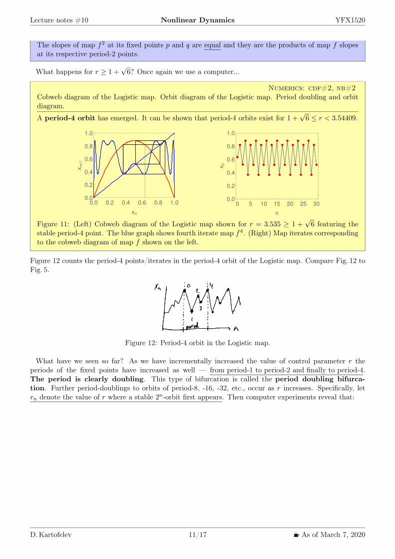
Lecture notes 10 Nonlinear Dynamics YFX1520
The slopes of map f2 at its fixed points p and q are equal and they are the products of map f slopesat its respective period-2 points
What happens for r ge 1 +radic6 Once again we use a computer
Numerics cdf2 nb2Cobweb diagram of the Logistic map Orbit diagram of the Logistic map Period doubling and orbitdiagram
A period-4 orbit has emerged It can be shown that period-4 orbits exist for 1 +radic6 le r lt 354409
00 02 04 06 08 1000
02
04
06
08
10
xn
xn+1
0 5 10 15 20 25 3000
02
04
06
08
10
n
xn
Figure 11 (Left) Cobweb diagram of the Logistic map shown for r = 3535 ge 1 +radic6 featuring the
stable period-4 point The blue graph shows fourth iterate map f4 (Right) Map iterates correspondingto the cobweb diagram of map f shown on the left
Figure 12 counts the period-4 pointsiterates in the period-4 orbit of the Logistic map Compare Fig 12 toFig 5
Figure 12 Period-4 orbit in the Logistic map
What have we seen so far As we have incrementally increased the value of control parameter r theperiods of the fixed points have increased as well mdash from period-1 to period-2 and finally to period-4The period is clearly doubling This type of bifurcation is called the period doubling bifurca-tion Further period-doublings to orbits of period-8 -16 -32 etc occur as r increases Specifically letrn denote the value of r where a stable 2n-orbit first appears Then computer experiments reveal that
D Kartofelev 1117 1003211 As of March 7 2020
Lecture notes 10 Nonlinear Dynamics YFX1520
Slide 10
Logistic map period doubling
Even number periods
rn ndash bifurcation point onset of stable period-2n orbit
r1 = 30 period-2r2 = 1 +
p6 344949 period-4
r3 354409 period-8r4 356441 period-16r5 356875 period-32r6 356969 period-64
r1 3569946 period-21
r1 ndash onset of chaos (the accumulation point)
= limn1
rn1 rn2
rn rn1 4669201609 (15)
DKartofelev YFX1520 10 18
Note that the successive bifurcations come faster and faster Ultimately the rn converge toa limiting value rinfin The convergence is (essentially) geometric (itrsquos geometric near rinfin) in the limitof large n the distance between successive transitions shrinks by a constant factor of δ This ratio iscalled the Feigenbaum constant After the accumulation point r gt rinfin the dynamics becomeschaotic as wersquoll see below
33 Orbit diagram
The orbit diagram is also called the fig tree diagram (Feigenbaum in German means ldquofig treerdquo) or (in-correctly) the Feigenbaum diagram You might guess that the system would become more and morechaotic for r gt rinfin as r increases but in fact the dynamics are more subtle than that To see the long-termbehaviour for all values of r at once we plot the orbit diagram a special kind of bifurcation diagramOrbit diagram plots the systemrsquos attractor (stable fixed points and stable period-p points) as a function ofcontrol parameter r
To generate the orbit diagram for yourself yoursquoll need to write a computer program with two loops Firstchoose a value of r Then generate an orbit starting from some random initial condition x0 Iterate for 300cycles or so to allow the system to settle down to its eventual stable behaviour Once the transients havedecayed plot many points say x301 x900 above that r Then move to an adjacent value of r and repeateventually sweeping across the whole diagram
The following interactive numerical file shows the orbit diagram for the Logistic map
Numerics cdf2 nb2Cobweb diagram of the Logistic map Orbit diagram of the Logistic map Period doubling and orbitdiagram
The connection between the cobweb diagram orbit diagram and the Lyapunov exponent is shown in theinteractive numerical file linked below
Numerics cdf3 nb3Logistic map cobweb diagram orbit diagram and map iterates Lyapunov exponent
D Kartofelev 1217 1003211 As of March 7 2020
Lecture notes 10 Nonlinear Dynamics YFX1520
Slides 11 12
Orbit diagram and period doubling
DKartofelev YFX1520 11 18
Zooming into the Logistic map self-similarity
No embedded video files in this pdf
DKartofelev YFX1520 12 18
The period doubling is driven by the subsequent flip bifurcations or supercritical pitchforkbifurcations (if we use the nomenclature introduced in Lecture 2) The unstable fixed point andperiod-p points are omitted from the orbit diagram
Feigenbaum diagram shows both stable and unstable fixed points and period-p points or simplydiagram branches (not shown here)
The orbit diagram of the Logistic map features self-similarity In mathematics a self-similarobject is (exactly or) approximately similar to a part of itself ie the whole has the same shape orquality as one or more of its sub-parts
34 Tangent bifurcation and odd number period-p points
Can an odd number period appear in the Logistic map mdash eg period-3 point One of the most intriguingfeatures of the orbit diagram is the occurrence of periodic windows for r gt rinfin The period-3 windowthat occurs for 1 +
radic8 le r le 38415 is the most conspicuous Suddenly against a backdrop of chaos a
stable period-3 orbit appears out of the blueLetrsquos see if we can find the period-3 window of Logistic map using a computer
Numerics cdf2 nb2Cobweb diagram of the Logistic map Orbit diagram of the Logistic map Period doubling and orbitdiagram
The tangent bifurcation is a new type of bifurcation for us that occurs at r = 1 +radic8
00 02 04 06 08 1000
02
04
06
08
10
xn
xn+1
0 5 10 15 20 25 3000
02
04
06
08
10
n
xn
Figure 13 (Left) Period-3 orbit of map f can be found in the period-3 window Here showing thetrajectory for r = 383 (Right) Map iterates corresponding to the cobweb diagram of map f shownon the left
The mechanism responsible for the occurrence of the odd number periods-p points is shown in Fig 14The intersections between the graph of f3 shown in red and the diagonal correspond to solutions of
D Kartofelev 1317 1003211 As of March 7 2020
Lecture notes 10 Nonlinear Dynamics YFX1520
Figure 14 Period-3 orbit can be found in period-3 window of the orbit diagram
f3(x) = x There are eight solutions for r ge 1+radic8 six of interest to us are marked with the blue dots and
two imposters that are not genuine period-3 they are actually fixed points or period-1 points for whichf(xlowast) = xlowast The blue filled dots in Fig 14 correspond to a stable period-3 cycle note that the slope off3(x) is shallow at these points consistent with the stability of the cycle In contrast the slope exceeds 1at the cycle marked by the empty blue dots this period-3 orbit is therefore unstable
Now suppose we decrease r toward the chaotic regime r lt 1+radic8 Then the red graph in Fig 14 changes
shape mdash the hill moves down and the valleys rise up The curve therefore moves towards the diagonalFigure 14 shows that when r = 1 +
radic8 the six blue intersections have merged to form three black filled
period-3 points by becoming tangent to the diagonal At this critical value of r the stable and unstableperiod-3 cycles coalesce and annihilate in a tangent bifurcation This transition defines the beginning ofthe periodic period-3 window
All odd number periods will also undergo the period doubling This means that all number periods [1infin)are eventually represented in the orbit diagram
Figure 14 also explains the self-similarity present in the orbit diagram as shown on Slide 12 for differentscales of magnification The peaks and valley of map f3 are smaller distorted copies of the original mapf Thus the local dynamics of the cobweb trajectories for map f3 must be similar to the dynamics of theoriginal map f
Slide 13
Intermittency3and period-3 window
Transient chaos and intermittency in dynamical systemsTangent bifurcation occurs at r = 1 +
p8 38284 (period-3 orbit)
50 100 150n
02
04
06
08
10xn
Iterates of Logistic map shown for r = 38282 and x0 = 015
3See Mathematica nb file uploaded to course webpageDKartofelev YFX1520 13 18
The dynamics closely related to the tangent bifurcation is intermittency Logistic map exhibitsintermittent chaos for r values just before the period-3 window
D Kartofelev 1417 1003211 As of March 7 2020
Lecture notes 10 Nonlinear Dynamics YFX1520
Numerics cdf4 nb4Period-3 window and intermittency in the Logistic map (iterates xn)
4 Sine map and universality of period doubling
It can be shown that in all unimodal maps same dynamics of period doubling occurs For example weconsider the sine map
Slide 14
Universality of period doubling in unimodal maps
1-D sine map4 The sine map has the form
xn+1 = r sin(xn) x0 2 [0 1] r 2 [0 1] n 2 Z+ (16)
where r is the control parameter
Read Mitchell J Feigenbaum ldquoQuantitative universality for a classof nonlinear transformationsrdquo Journal of Statistical Physics 19(1)pp 25ndash52 1978 doi101007BF01020332
Read Mitchell J Feigenbaum ldquoUniversal behavior in nonlinearsystemsrdquo Physica D Nonlinear Phenomena 7(1ndash3) pp 16ndash391983 doi1010160167-2789(83)90112-4
4See Mathematica nb file (cobweb diagram and orbit diagram) uploaded tothe course webpage
DKartofelev YFX1520 14 18
The graph of the sine map has the same basic shape as the graph of the Logistic map Both curvesare smooth concave down and have a single maximum Such maps are called unimodal
Sine is also a transcendental function opposed to an algebraic function as is the polynomial thatdescribes the Logistic map A transcendental function is an analytic function that does not satisfy apolynomial equation In other words a transcendental function ldquotranscendsrdquo algebra in that it cannotbe expressed in terms of a finite sequence of the algebraic operations of addition multiplication androot extraction
The transcendental nature of the sine map must makes the underlying higher-dimensional physicsrepresented by the sine map fundamentally different from eg the three-dimensional Lorenz flowsampled by Lorenz map
Letrsquos study the dynamics of the sine map using a computer
Numerics cdf5 nb5The sine map iterates cobweb and orbit diagrams (xn isin [0 1])
Numerics cdf6 nb6The sine map iterates cobweb and orbit diagrams (xn isin [minus1 1])
The dynamics is surprisingly similar to the dynamics of the Logistic map Mitchell J Feigenbaumwas first to discover the quantitative laws that are independent of unimodal map functions f Bythat we mean that the algebraic form of f(x) is irrelevant only its overall shape matters
D Kartofelev 1517 1003211 As of March 7 2020
Lecture notes 10 Nonlinear Dynamics YFX1520
Slide 151-D unimodal maps and Feigenbaum constants
= limn1
n1
n= lim
n1
rn1 rn2
rn rn1 4669201609 (17)
crarr = limn1
dn1
dn 2502907875 (18)
DKartofelev YFX1520 15 18
Here xm = max f(x) is the maximum of the map graph The Feigenbaum constants are valid up tothe onset of chaos at rinfin and inside each periodic window for r gt rinfin
In addition to scaling law in control parameter r direction shown earlier Feigenbaum also foundscaling law for the vertical x-direction of the orbit diagram The Feigenbaum constants are uni-versal the same convergence rate appears no matter what unimodal map is iterated They are newmathematical constants as basic to period doubling as π is to circles
Reading suggestion
Link File name CitationPaper2 paper3pdf Mitchell J Feigenbaum ldquoQuantitative universality for a class of nonlinear trans-
formationsrdquo Journal of Statistical Physics 19(1) pp 25ndash52 (1978)doi101007BF01020332
Paper3 paper4pdf Mitchell J Feigenbaum ldquoUniversal behavior in nonlinear systemsrdquo Physica DNonlinear Phenomena 7(1ndash3) pp 16ndash39 (1983)doi1010160167-2789(83)90112-4
5 Universal route to chaos
We showed that the qualitative dynamics of the Logistic and sine maps are identical They both undergoperiod doubling routes to chaos followed by periodic windows interwoven with chaotic bandsEven more remarkably the periodic windows occur in the same order and with the same relative sizes Forinstance the period-3 window is the largest in both cases and the next largest windows preceding it areperiod-5 and period-6 But there are quantitative differences For instance the period doubling bifurcationsoccur later (for greater parameter r value) in the Logistic map and the periodic windows are thinner
Turns out that the onset of chaos via period doubling is predominant in nature and in artificial chaoticsystems Feigenbaum constants have real predictive power in various scientific applications The perioddoubling bifurcation is the ldquorouterdquo taken by nonlinear systems to reach chaotic solution Interm of the bifurcations introduced in Lecture 2 the period doubling bifurcation can also be seen as a seriesof subsequentsucceeding supercritical pitchfork bifurcations see Slide 11
Revision questions
1 What is cobweb diagram2 What is recurrence map or recurrence relation3 What is 1-D map4 How to find fixed points of 1-D maps5 What is Lorenz map
D Kartofelev 1617 1003211 As of March 7 2020
Lecture notes 10 Nonlinear Dynamics YFX1520
6 What is Logistic map7 What is sine map8 What is period doubling9 What is period doubling bifurcation
10 What is tangent bifurcation11 Do odd number periods (period-p orbits) exist in chaotic systems12 Do even number periods (period-p orbits) exist in chaotic systems13 Can maps produce transient chaos14 Can maps produce intermittency15 Can maps produce intermittent chaos16 What is orbit diagram (or Feigenbaum diagram)17 What are Feigenbaum constants
D Kartofelev 1717 1003211 As of March 7 2020
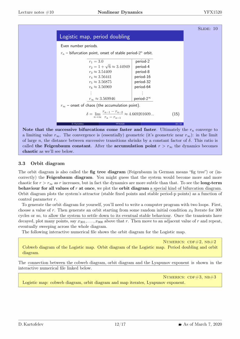
Lecture notes 10 Nonlinear Dynamics YFX1520
Slide 10
Logistic map period doubling
Even number periods
rn ndash bifurcation point onset of stable period-2n orbit
r1 = 30 period-2r2 = 1 +
p6 344949 period-4
r3 354409 period-8r4 356441 period-16r5 356875 period-32r6 356969 period-64
r1 3569946 period-21
r1 ndash onset of chaos (the accumulation point)
= limn1
rn1 rn2
rn rn1 4669201609 (15)
DKartofelev YFX1520 10 18
Note that the successive bifurcations come faster and faster Ultimately the rn converge toa limiting value rinfin The convergence is (essentially) geometric (itrsquos geometric near rinfin) in the limitof large n the distance between successive transitions shrinks by a constant factor of δ This ratio iscalled the Feigenbaum constant After the accumulation point r gt rinfin the dynamics becomeschaotic as wersquoll see below
33 Orbit diagram
The orbit diagram is also called the fig tree diagram (Feigenbaum in German means ldquofig treerdquo) or (in-correctly) the Feigenbaum diagram You might guess that the system would become more and morechaotic for r gt rinfin as r increases but in fact the dynamics are more subtle than that To see the long-termbehaviour for all values of r at once we plot the orbit diagram a special kind of bifurcation diagramOrbit diagram plots the systemrsquos attractor (stable fixed points and stable period-p points) as a function ofcontrol parameter r
To generate the orbit diagram for yourself yoursquoll need to write a computer program with two loops Firstchoose a value of r Then generate an orbit starting from some random initial condition x0 Iterate for 300cycles or so to allow the system to settle down to its eventual stable behaviour Once the transients havedecayed plot many points say x301 x900 above that r Then move to an adjacent value of r and repeateventually sweeping across the whole diagram
The following interactive numerical file shows the orbit diagram for the Logistic map
Numerics cdf2 nb2Cobweb diagram of the Logistic map Orbit diagram of the Logistic map Period doubling and orbitdiagram
The connection between the cobweb diagram orbit diagram and the Lyapunov exponent is shown in theinteractive numerical file linked below
Numerics cdf3 nb3Logistic map cobweb diagram orbit diagram and map iterates Lyapunov exponent
D Kartofelev 1217 1003211 As of March 7 2020
Lecture notes 10 Nonlinear Dynamics YFX1520
Slides 11 12
Orbit diagram and period doubling
DKartofelev YFX1520 11 18
Zooming into the Logistic map self-similarity
No embedded video files in this pdf
DKartofelev YFX1520 12 18
The period doubling is driven by the subsequent flip bifurcations or supercritical pitchforkbifurcations (if we use the nomenclature introduced in Lecture 2) The unstable fixed point andperiod-p points are omitted from the orbit diagram
Feigenbaum diagram shows both stable and unstable fixed points and period-p points or simplydiagram branches (not shown here)
The orbit diagram of the Logistic map features self-similarity In mathematics a self-similarobject is (exactly or) approximately similar to a part of itself ie the whole has the same shape orquality as one or more of its sub-parts
34 Tangent bifurcation and odd number period-p points
Can an odd number period appear in the Logistic map mdash eg period-3 point One of the most intriguingfeatures of the orbit diagram is the occurrence of periodic windows for r gt rinfin The period-3 windowthat occurs for 1 +
radic8 le r le 38415 is the most conspicuous Suddenly against a backdrop of chaos a
stable period-3 orbit appears out of the blueLetrsquos see if we can find the period-3 window of Logistic map using a computer
Numerics cdf2 nb2Cobweb diagram of the Logistic map Orbit diagram of the Logistic map Period doubling and orbitdiagram
The tangent bifurcation is a new type of bifurcation for us that occurs at r = 1 +radic8
00 02 04 06 08 1000
02
04
06
08
10
xn
xn+1
0 5 10 15 20 25 3000
02
04
06
08
10
n
xn
Figure 13 (Left) Period-3 orbit of map f can be found in the period-3 window Here showing thetrajectory for r = 383 (Right) Map iterates corresponding to the cobweb diagram of map f shownon the left
The mechanism responsible for the occurrence of the odd number periods-p points is shown in Fig 14The intersections between the graph of f3 shown in red and the diagonal correspond to solutions of
D Kartofelev 1317 1003211 As of March 7 2020
Lecture notes 10 Nonlinear Dynamics YFX1520
Figure 14 Period-3 orbit can be found in period-3 window of the orbit diagram
f3(x) = x There are eight solutions for r ge 1+radic8 six of interest to us are marked with the blue dots and
two imposters that are not genuine period-3 they are actually fixed points or period-1 points for whichf(xlowast) = xlowast The blue filled dots in Fig 14 correspond to a stable period-3 cycle note that the slope off3(x) is shallow at these points consistent with the stability of the cycle In contrast the slope exceeds 1at the cycle marked by the empty blue dots this period-3 orbit is therefore unstable
Now suppose we decrease r toward the chaotic regime r lt 1+radic8 Then the red graph in Fig 14 changes
shape mdash the hill moves down and the valleys rise up The curve therefore moves towards the diagonalFigure 14 shows that when r = 1 +
radic8 the six blue intersections have merged to form three black filled
period-3 points by becoming tangent to the diagonal At this critical value of r the stable and unstableperiod-3 cycles coalesce and annihilate in a tangent bifurcation This transition defines the beginning ofthe periodic period-3 window
All odd number periods will also undergo the period doubling This means that all number periods [1infin)are eventually represented in the orbit diagram
Figure 14 also explains the self-similarity present in the orbit diagram as shown on Slide 12 for differentscales of magnification The peaks and valley of map f3 are smaller distorted copies of the original mapf Thus the local dynamics of the cobweb trajectories for map f3 must be similar to the dynamics of theoriginal map f
Slide 13
Intermittency3and period-3 window
Transient chaos and intermittency in dynamical systemsTangent bifurcation occurs at r = 1 +
p8 38284 (period-3 orbit)
50 100 150n
02
04
06
08
10xn
Iterates of Logistic map shown for r = 38282 and x0 = 015
3See Mathematica nb file uploaded to course webpageDKartofelev YFX1520 13 18
The dynamics closely related to the tangent bifurcation is intermittency Logistic map exhibitsintermittent chaos for r values just before the period-3 window
D Kartofelev 1417 1003211 As of March 7 2020
Lecture notes 10 Nonlinear Dynamics YFX1520
Numerics cdf4 nb4Period-3 window and intermittency in the Logistic map (iterates xn)
4 Sine map and universality of period doubling
It can be shown that in all unimodal maps same dynamics of period doubling occurs For example weconsider the sine map
Slide 14
Universality of period doubling in unimodal maps
1-D sine map4 The sine map has the form
xn+1 = r sin(xn) x0 2 [0 1] r 2 [0 1] n 2 Z+ (16)
where r is the control parameter
Read Mitchell J Feigenbaum ldquoQuantitative universality for a classof nonlinear transformationsrdquo Journal of Statistical Physics 19(1)pp 25ndash52 1978 doi101007BF01020332
Read Mitchell J Feigenbaum ldquoUniversal behavior in nonlinearsystemsrdquo Physica D Nonlinear Phenomena 7(1ndash3) pp 16ndash391983 doi1010160167-2789(83)90112-4
4See Mathematica nb file (cobweb diagram and orbit diagram) uploaded tothe course webpage
DKartofelev YFX1520 14 18
The graph of the sine map has the same basic shape as the graph of the Logistic map Both curvesare smooth concave down and have a single maximum Such maps are called unimodal
Sine is also a transcendental function opposed to an algebraic function as is the polynomial thatdescribes the Logistic map A transcendental function is an analytic function that does not satisfy apolynomial equation In other words a transcendental function ldquotranscendsrdquo algebra in that it cannotbe expressed in terms of a finite sequence of the algebraic operations of addition multiplication androot extraction
The transcendental nature of the sine map must makes the underlying higher-dimensional physicsrepresented by the sine map fundamentally different from eg the three-dimensional Lorenz flowsampled by Lorenz map
Letrsquos study the dynamics of the sine map using a computer
Numerics cdf5 nb5The sine map iterates cobweb and orbit diagrams (xn isin [0 1])
Numerics cdf6 nb6The sine map iterates cobweb and orbit diagrams (xn isin [minus1 1])
The dynamics is surprisingly similar to the dynamics of the Logistic map Mitchell J Feigenbaumwas first to discover the quantitative laws that are independent of unimodal map functions f Bythat we mean that the algebraic form of f(x) is irrelevant only its overall shape matters
D Kartofelev 1517 1003211 As of March 7 2020
Lecture notes 10 Nonlinear Dynamics YFX1520
Slide 151-D unimodal maps and Feigenbaum constants
= limn1
n1
n= lim
n1
rn1 rn2
rn rn1 4669201609 (17)
crarr = limn1
dn1
dn 2502907875 (18)
DKartofelev YFX1520 15 18
Here xm = max f(x) is the maximum of the map graph The Feigenbaum constants are valid up tothe onset of chaos at rinfin and inside each periodic window for r gt rinfin
In addition to scaling law in control parameter r direction shown earlier Feigenbaum also foundscaling law for the vertical x-direction of the orbit diagram The Feigenbaum constants are uni-versal the same convergence rate appears no matter what unimodal map is iterated They are newmathematical constants as basic to period doubling as π is to circles
Reading suggestion
Link File name CitationPaper2 paper3pdf Mitchell J Feigenbaum ldquoQuantitative universality for a class of nonlinear trans-
formationsrdquo Journal of Statistical Physics 19(1) pp 25ndash52 (1978)doi101007BF01020332
Paper3 paper4pdf Mitchell J Feigenbaum ldquoUniversal behavior in nonlinear systemsrdquo Physica DNonlinear Phenomena 7(1ndash3) pp 16ndash39 (1983)doi1010160167-2789(83)90112-4
5 Universal route to chaos
We showed that the qualitative dynamics of the Logistic and sine maps are identical They both undergoperiod doubling routes to chaos followed by periodic windows interwoven with chaotic bandsEven more remarkably the periodic windows occur in the same order and with the same relative sizes Forinstance the period-3 window is the largest in both cases and the next largest windows preceding it areperiod-5 and period-6 But there are quantitative differences For instance the period doubling bifurcationsoccur later (for greater parameter r value) in the Logistic map and the periodic windows are thinner
Turns out that the onset of chaos via period doubling is predominant in nature and in artificial chaoticsystems Feigenbaum constants have real predictive power in various scientific applications The perioddoubling bifurcation is the ldquorouterdquo taken by nonlinear systems to reach chaotic solution Interm of the bifurcations introduced in Lecture 2 the period doubling bifurcation can also be seen as a seriesof subsequentsucceeding supercritical pitchfork bifurcations see Slide 11
Revision questions
1 What is cobweb diagram2 What is recurrence map or recurrence relation3 What is 1-D map4 How to find fixed points of 1-D maps5 What is Lorenz map
D Kartofelev 1617 1003211 As of March 7 2020
Lecture notes 10 Nonlinear Dynamics YFX1520
6 What is Logistic map7 What is sine map8 What is period doubling9 What is period doubling bifurcation
10 What is tangent bifurcation11 Do odd number periods (period-p orbits) exist in chaotic systems12 Do even number periods (period-p orbits) exist in chaotic systems13 Can maps produce transient chaos14 Can maps produce intermittency15 Can maps produce intermittent chaos16 What is orbit diagram (or Feigenbaum diagram)17 What are Feigenbaum constants
D Kartofelev 1717 1003211 As of March 7 2020
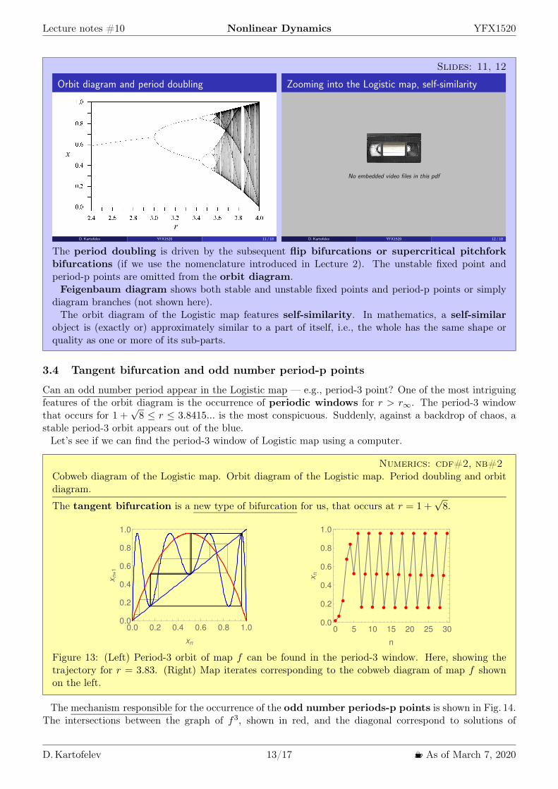
Lecture notes 10 Nonlinear Dynamics YFX1520
Slides 11 12
Orbit diagram and period doubling
DKartofelev YFX1520 11 18
Zooming into the Logistic map self-similarity
No embedded video files in this pdf
DKartofelev YFX1520 12 18
The period doubling is driven by the subsequent flip bifurcations or supercritical pitchforkbifurcations (if we use the nomenclature introduced in Lecture 2) The unstable fixed point andperiod-p points are omitted from the orbit diagram
Feigenbaum diagram shows both stable and unstable fixed points and period-p points or simplydiagram branches (not shown here)
The orbit diagram of the Logistic map features self-similarity In mathematics a self-similarobject is (exactly or) approximately similar to a part of itself ie the whole has the same shape orquality as one or more of its sub-parts
34 Tangent bifurcation and odd number period-p points
Can an odd number period appear in the Logistic map mdash eg period-3 point One of the most intriguingfeatures of the orbit diagram is the occurrence of periodic windows for r gt rinfin The period-3 windowthat occurs for 1 +
radic8 le r le 38415 is the most conspicuous Suddenly against a backdrop of chaos a
stable period-3 orbit appears out of the blueLetrsquos see if we can find the period-3 window of Logistic map using a computer
Numerics cdf2 nb2Cobweb diagram of the Logistic map Orbit diagram of the Logistic map Period doubling and orbitdiagram
The tangent bifurcation is a new type of bifurcation for us that occurs at r = 1 +radic8
00 02 04 06 08 1000
02
04
06
08
10
xn
xn+1
0 5 10 15 20 25 3000
02
04
06
08
10
n
xn
Figure 13 (Left) Period-3 orbit of map f can be found in the period-3 window Here showing thetrajectory for r = 383 (Right) Map iterates corresponding to the cobweb diagram of map f shownon the left
The mechanism responsible for the occurrence of the odd number periods-p points is shown in Fig 14The intersections between the graph of f3 shown in red and the diagonal correspond to solutions of
D Kartofelev 1317 1003211 As of March 7 2020
Lecture notes 10 Nonlinear Dynamics YFX1520
Figure 14 Period-3 orbit can be found in period-3 window of the orbit diagram
f3(x) = x There are eight solutions for r ge 1+radic8 six of interest to us are marked with the blue dots and
two imposters that are not genuine period-3 they are actually fixed points or period-1 points for whichf(xlowast) = xlowast The blue filled dots in Fig 14 correspond to a stable period-3 cycle note that the slope off3(x) is shallow at these points consistent with the stability of the cycle In contrast the slope exceeds 1at the cycle marked by the empty blue dots this period-3 orbit is therefore unstable
Now suppose we decrease r toward the chaotic regime r lt 1+radic8 Then the red graph in Fig 14 changes
shape mdash the hill moves down and the valleys rise up The curve therefore moves towards the diagonalFigure 14 shows that when r = 1 +
radic8 the six blue intersections have merged to form three black filled
period-3 points by becoming tangent to the diagonal At this critical value of r the stable and unstableperiod-3 cycles coalesce and annihilate in a tangent bifurcation This transition defines the beginning ofthe periodic period-3 window
All odd number periods will also undergo the period doubling This means that all number periods [1infin)are eventually represented in the orbit diagram
Figure 14 also explains the self-similarity present in the orbit diagram as shown on Slide 12 for differentscales of magnification The peaks and valley of map f3 are smaller distorted copies of the original mapf Thus the local dynamics of the cobweb trajectories for map f3 must be similar to the dynamics of theoriginal map f
Slide 13
Intermittency3and period-3 window
Transient chaos and intermittency in dynamical systemsTangent bifurcation occurs at r = 1 +
p8 38284 (period-3 orbit)
50 100 150n
02
04
06
08
10xn
Iterates of Logistic map shown for r = 38282 and x0 = 015
3See Mathematica nb file uploaded to course webpageDKartofelev YFX1520 13 18
The dynamics closely related to the tangent bifurcation is intermittency Logistic map exhibitsintermittent chaos for r values just before the period-3 window
D Kartofelev 1417 1003211 As of March 7 2020
Lecture notes 10 Nonlinear Dynamics YFX1520
Numerics cdf4 nb4Period-3 window and intermittency in the Logistic map (iterates xn)
4 Sine map and universality of period doubling
It can be shown that in all unimodal maps same dynamics of period doubling occurs For example weconsider the sine map
Slide 14
Universality of period doubling in unimodal maps
1-D sine map4 The sine map has the form
xn+1 = r sin(xn) x0 2 [0 1] r 2 [0 1] n 2 Z+ (16)
where r is the control parameter
Read Mitchell J Feigenbaum ldquoQuantitative universality for a classof nonlinear transformationsrdquo Journal of Statistical Physics 19(1)pp 25ndash52 1978 doi101007BF01020332
Read Mitchell J Feigenbaum ldquoUniversal behavior in nonlinearsystemsrdquo Physica D Nonlinear Phenomena 7(1ndash3) pp 16ndash391983 doi1010160167-2789(83)90112-4
4See Mathematica nb file (cobweb diagram and orbit diagram) uploaded tothe course webpage
DKartofelev YFX1520 14 18
The graph of the sine map has the same basic shape as the graph of the Logistic map Both curvesare smooth concave down and have a single maximum Such maps are called unimodal
Sine is also a transcendental function opposed to an algebraic function as is the polynomial thatdescribes the Logistic map A transcendental function is an analytic function that does not satisfy apolynomial equation In other words a transcendental function ldquotranscendsrdquo algebra in that it cannotbe expressed in terms of a finite sequence of the algebraic operations of addition multiplication androot extraction
The transcendental nature of the sine map must makes the underlying higher-dimensional physicsrepresented by the sine map fundamentally different from eg the three-dimensional Lorenz flowsampled by Lorenz map
Letrsquos study the dynamics of the sine map using a computer
Numerics cdf5 nb5The sine map iterates cobweb and orbit diagrams (xn isin [0 1])
Numerics cdf6 nb6The sine map iterates cobweb and orbit diagrams (xn isin [minus1 1])
The dynamics is surprisingly similar to the dynamics of the Logistic map Mitchell J Feigenbaumwas first to discover the quantitative laws that are independent of unimodal map functions f Bythat we mean that the algebraic form of f(x) is irrelevant only its overall shape matters
D Kartofelev 1517 1003211 As of March 7 2020
Lecture notes 10 Nonlinear Dynamics YFX1520
Slide 151-D unimodal maps and Feigenbaum constants
= limn1
n1
n= lim
n1
rn1 rn2
rn rn1 4669201609 (17)
crarr = limn1
dn1
dn 2502907875 (18)
DKartofelev YFX1520 15 18
Here xm = max f(x) is the maximum of the map graph The Feigenbaum constants are valid up tothe onset of chaos at rinfin and inside each periodic window for r gt rinfin
In addition to scaling law in control parameter r direction shown earlier Feigenbaum also foundscaling law for the vertical x-direction of the orbit diagram The Feigenbaum constants are uni-versal the same convergence rate appears no matter what unimodal map is iterated They are newmathematical constants as basic to period doubling as π is to circles
Reading suggestion
Link File name CitationPaper2 paper3pdf Mitchell J Feigenbaum ldquoQuantitative universality for a class of nonlinear trans-
formationsrdquo Journal of Statistical Physics 19(1) pp 25ndash52 (1978)doi101007BF01020332
Paper3 paper4pdf Mitchell J Feigenbaum ldquoUniversal behavior in nonlinear systemsrdquo Physica DNonlinear Phenomena 7(1ndash3) pp 16ndash39 (1983)doi1010160167-2789(83)90112-4
5 Universal route to chaos
We showed that the qualitative dynamics of the Logistic and sine maps are identical They both undergoperiod doubling routes to chaos followed by periodic windows interwoven with chaotic bandsEven more remarkably the periodic windows occur in the same order and with the same relative sizes Forinstance the period-3 window is the largest in both cases and the next largest windows preceding it areperiod-5 and period-6 But there are quantitative differences For instance the period doubling bifurcationsoccur later (for greater parameter r value) in the Logistic map and the periodic windows are thinner
Turns out that the onset of chaos via period doubling is predominant in nature and in artificial chaoticsystems Feigenbaum constants have real predictive power in various scientific applications The perioddoubling bifurcation is the ldquorouterdquo taken by nonlinear systems to reach chaotic solution Interm of the bifurcations introduced in Lecture 2 the period doubling bifurcation can also be seen as a seriesof subsequentsucceeding supercritical pitchfork bifurcations see Slide 11
Revision questions
1 What is cobweb diagram2 What is recurrence map or recurrence relation3 What is 1-D map4 How to find fixed points of 1-D maps5 What is Lorenz map
D Kartofelev 1617 1003211 As of March 7 2020
Lecture notes 10 Nonlinear Dynamics YFX1520
6 What is Logistic map7 What is sine map8 What is period doubling9 What is period doubling bifurcation
10 What is tangent bifurcation11 Do odd number periods (period-p orbits) exist in chaotic systems12 Do even number periods (period-p orbits) exist in chaotic systems13 Can maps produce transient chaos14 Can maps produce intermittency15 Can maps produce intermittent chaos16 What is orbit diagram (or Feigenbaum diagram)17 What are Feigenbaum constants
D Kartofelev 1717 1003211 As of March 7 2020
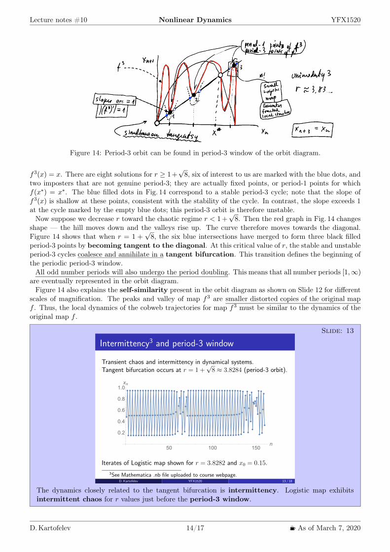
Lecture notes 10 Nonlinear Dynamics YFX1520
Figure 14 Period-3 orbit can be found in period-3 window of the orbit diagram
f3(x) = x There are eight solutions for r ge 1+radic8 six of interest to us are marked with the blue dots and
two imposters that are not genuine period-3 they are actually fixed points or period-1 points for whichf(xlowast) = xlowast The blue filled dots in Fig 14 correspond to a stable period-3 cycle note that the slope off3(x) is shallow at these points consistent with the stability of the cycle In contrast the slope exceeds 1at the cycle marked by the empty blue dots this period-3 orbit is therefore unstable
Now suppose we decrease r toward the chaotic regime r lt 1+radic8 Then the red graph in Fig 14 changes
shape mdash the hill moves down and the valleys rise up The curve therefore moves towards the diagonalFigure 14 shows that when r = 1 +
radic8 the six blue intersections have merged to form three black filled
period-3 points by becoming tangent to the diagonal At this critical value of r the stable and unstableperiod-3 cycles coalesce and annihilate in a tangent bifurcation This transition defines the beginning ofthe periodic period-3 window
All odd number periods will also undergo the period doubling This means that all number periods [1infin)are eventually represented in the orbit diagram
Figure 14 also explains the self-similarity present in the orbit diagram as shown on Slide 12 for differentscales of magnification The peaks and valley of map f3 are smaller distorted copies of the original mapf Thus the local dynamics of the cobweb trajectories for map f3 must be similar to the dynamics of theoriginal map f
Slide 13
Intermittency3and period-3 window
Transient chaos and intermittency in dynamical systemsTangent bifurcation occurs at r = 1 +
p8 38284 (period-3 orbit)
50 100 150n
02
04
06
08
10xn
Iterates of Logistic map shown for r = 38282 and x0 = 015
3See Mathematica nb file uploaded to course webpageDKartofelev YFX1520 13 18
The dynamics closely related to the tangent bifurcation is intermittency Logistic map exhibitsintermittent chaos for r values just before the period-3 window
D Kartofelev 1417 1003211 As of March 7 2020
Lecture notes 10 Nonlinear Dynamics YFX1520
Numerics cdf4 nb4Period-3 window and intermittency in the Logistic map (iterates xn)
4 Sine map and universality of period doubling
It can be shown that in all unimodal maps same dynamics of period doubling occurs For example weconsider the sine map
Slide 14
Universality of period doubling in unimodal maps
1-D sine map4 The sine map has the form
xn+1 = r sin(xn) x0 2 [0 1] r 2 [0 1] n 2 Z+ (16)
where r is the control parameter
Read Mitchell J Feigenbaum ldquoQuantitative universality for a classof nonlinear transformationsrdquo Journal of Statistical Physics 19(1)pp 25ndash52 1978 doi101007BF01020332
Read Mitchell J Feigenbaum ldquoUniversal behavior in nonlinearsystemsrdquo Physica D Nonlinear Phenomena 7(1ndash3) pp 16ndash391983 doi1010160167-2789(83)90112-4
4See Mathematica nb file (cobweb diagram and orbit diagram) uploaded tothe course webpage
DKartofelev YFX1520 14 18
The graph of the sine map has the same basic shape as the graph of the Logistic map Both curvesare smooth concave down and have a single maximum Such maps are called unimodal
Sine is also a transcendental function opposed to an algebraic function as is the polynomial thatdescribes the Logistic map A transcendental function is an analytic function that does not satisfy apolynomial equation In other words a transcendental function ldquotranscendsrdquo algebra in that it cannotbe expressed in terms of a finite sequence of the algebraic operations of addition multiplication androot extraction
The transcendental nature of the sine map must makes the underlying higher-dimensional physicsrepresented by the sine map fundamentally different from eg the three-dimensional Lorenz flowsampled by Lorenz map
Letrsquos study the dynamics of the sine map using a computer
Numerics cdf5 nb5The sine map iterates cobweb and orbit diagrams (xn isin [0 1])
Numerics cdf6 nb6The sine map iterates cobweb and orbit diagrams (xn isin [minus1 1])
The dynamics is surprisingly similar to the dynamics of the Logistic map Mitchell J Feigenbaumwas first to discover the quantitative laws that are independent of unimodal map functions f Bythat we mean that the algebraic form of f(x) is irrelevant only its overall shape matters
D Kartofelev 1517 1003211 As of March 7 2020
Lecture notes 10 Nonlinear Dynamics YFX1520
Slide 151-D unimodal maps and Feigenbaum constants
= limn1
n1
n= lim
n1
rn1 rn2
rn rn1 4669201609 (17)
crarr = limn1
dn1
dn 2502907875 (18)
DKartofelev YFX1520 15 18
Here xm = max f(x) is the maximum of the map graph The Feigenbaum constants are valid up tothe onset of chaos at rinfin and inside each periodic window for r gt rinfin
In addition to scaling law in control parameter r direction shown earlier Feigenbaum also foundscaling law for the vertical x-direction of the orbit diagram The Feigenbaum constants are uni-versal the same convergence rate appears no matter what unimodal map is iterated They are newmathematical constants as basic to period doubling as π is to circles
Reading suggestion
Link File name CitationPaper2 paper3pdf Mitchell J Feigenbaum ldquoQuantitative universality for a class of nonlinear trans-
formationsrdquo Journal of Statistical Physics 19(1) pp 25ndash52 (1978)doi101007BF01020332
Paper3 paper4pdf Mitchell J Feigenbaum ldquoUniversal behavior in nonlinear systemsrdquo Physica DNonlinear Phenomena 7(1ndash3) pp 16ndash39 (1983)doi1010160167-2789(83)90112-4
5 Universal route to chaos
We showed that the qualitative dynamics of the Logistic and sine maps are identical They both undergoperiod doubling routes to chaos followed by periodic windows interwoven with chaotic bandsEven more remarkably the periodic windows occur in the same order and with the same relative sizes Forinstance the period-3 window is the largest in both cases and the next largest windows preceding it areperiod-5 and period-6 But there are quantitative differences For instance the period doubling bifurcationsoccur later (for greater parameter r value) in the Logistic map and the periodic windows are thinner
Turns out that the onset of chaos via period doubling is predominant in nature and in artificial chaoticsystems Feigenbaum constants have real predictive power in various scientific applications The perioddoubling bifurcation is the ldquorouterdquo taken by nonlinear systems to reach chaotic solution Interm of the bifurcations introduced in Lecture 2 the period doubling bifurcation can also be seen as a seriesof subsequentsucceeding supercritical pitchfork bifurcations see Slide 11
Revision questions
1 What is cobweb diagram2 What is recurrence map or recurrence relation3 What is 1-D map4 How to find fixed points of 1-D maps5 What is Lorenz map
D Kartofelev 1617 1003211 As of March 7 2020
Lecture notes 10 Nonlinear Dynamics YFX1520
6 What is Logistic map7 What is sine map8 What is period doubling9 What is period doubling bifurcation
10 What is tangent bifurcation11 Do odd number periods (period-p orbits) exist in chaotic systems12 Do even number periods (period-p orbits) exist in chaotic systems13 Can maps produce transient chaos14 Can maps produce intermittency15 Can maps produce intermittent chaos16 What is orbit diagram (or Feigenbaum diagram)17 What are Feigenbaum constants
D Kartofelev 1717 1003211 As of March 7 2020
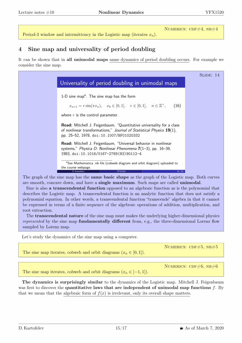
Lecture notes 10 Nonlinear Dynamics YFX1520
Numerics cdf4 nb4Period-3 window and intermittency in the Logistic map (iterates xn)
4 Sine map and universality of period doubling
It can be shown that in all unimodal maps same dynamics of period doubling occurs For example weconsider the sine map
Slide 14
Universality of period doubling in unimodal maps
1-D sine map4 The sine map has the form
xn+1 = r sin(xn) x0 2 [0 1] r 2 [0 1] n 2 Z+ (16)
where r is the control parameter
Read Mitchell J Feigenbaum ldquoQuantitative universality for a classof nonlinear transformationsrdquo Journal of Statistical Physics 19(1)pp 25ndash52 1978 doi101007BF01020332
Read Mitchell J Feigenbaum ldquoUniversal behavior in nonlinearsystemsrdquo Physica D Nonlinear Phenomena 7(1ndash3) pp 16ndash391983 doi1010160167-2789(83)90112-4
4See Mathematica nb file (cobweb diagram and orbit diagram) uploaded tothe course webpage
DKartofelev YFX1520 14 18
The graph of the sine map has the same basic shape as the graph of the Logistic map Both curvesare smooth concave down and have a single maximum Such maps are called unimodal
Sine is also a transcendental function opposed to an algebraic function as is the polynomial thatdescribes the Logistic map A transcendental function is an analytic function that does not satisfy apolynomial equation In other words a transcendental function ldquotranscendsrdquo algebra in that it cannotbe expressed in terms of a finite sequence of the algebraic operations of addition multiplication androot extraction
The transcendental nature of the sine map must makes the underlying higher-dimensional physicsrepresented by the sine map fundamentally different from eg the three-dimensional Lorenz flowsampled by Lorenz map
Letrsquos study the dynamics of the sine map using a computer
Numerics cdf5 nb5The sine map iterates cobweb and orbit diagrams (xn isin [0 1])
Numerics cdf6 nb6The sine map iterates cobweb and orbit diagrams (xn isin [minus1 1])
The dynamics is surprisingly similar to the dynamics of the Logistic map Mitchell J Feigenbaumwas first to discover the quantitative laws that are independent of unimodal map functions f Bythat we mean that the algebraic form of f(x) is irrelevant only its overall shape matters
D Kartofelev 1517 1003211 As of March 7 2020
Lecture notes 10 Nonlinear Dynamics YFX1520
Slide 151-D unimodal maps and Feigenbaum constants
= limn1
n1
n= lim
n1
rn1 rn2
rn rn1 4669201609 (17)
crarr = limn1
dn1
dn 2502907875 (18)
DKartofelev YFX1520 15 18
Here xm = max f(x) is the maximum of the map graph The Feigenbaum constants are valid up tothe onset of chaos at rinfin and inside each periodic window for r gt rinfin
In addition to scaling law in control parameter r direction shown earlier Feigenbaum also foundscaling law for the vertical x-direction of the orbit diagram The Feigenbaum constants are uni-versal the same convergence rate appears no matter what unimodal map is iterated They are newmathematical constants as basic to period doubling as π is to circles
Reading suggestion
Link File name CitationPaper2 paper3pdf Mitchell J Feigenbaum ldquoQuantitative universality for a class of nonlinear trans-
formationsrdquo Journal of Statistical Physics 19(1) pp 25ndash52 (1978)doi101007BF01020332
Paper3 paper4pdf Mitchell J Feigenbaum ldquoUniversal behavior in nonlinear systemsrdquo Physica DNonlinear Phenomena 7(1ndash3) pp 16ndash39 (1983)doi1010160167-2789(83)90112-4
5 Universal route to chaos
We showed that the qualitative dynamics of the Logistic and sine maps are identical They both undergoperiod doubling routes to chaos followed by periodic windows interwoven with chaotic bandsEven more remarkably the periodic windows occur in the same order and with the same relative sizes Forinstance the period-3 window is the largest in both cases and the next largest windows preceding it areperiod-5 and period-6 But there are quantitative differences For instance the period doubling bifurcationsoccur later (for greater parameter r value) in the Logistic map and the periodic windows are thinner
Turns out that the onset of chaos via period doubling is predominant in nature and in artificial chaoticsystems Feigenbaum constants have real predictive power in various scientific applications The perioddoubling bifurcation is the ldquorouterdquo taken by nonlinear systems to reach chaotic solution Interm of the bifurcations introduced in Lecture 2 the period doubling bifurcation can also be seen as a seriesof subsequentsucceeding supercritical pitchfork bifurcations see Slide 11
Revision questions
1 What is cobweb diagram2 What is recurrence map or recurrence relation3 What is 1-D map4 How to find fixed points of 1-D maps5 What is Lorenz map
D Kartofelev 1617 1003211 As of March 7 2020
Lecture notes 10 Nonlinear Dynamics YFX1520
6 What is Logistic map7 What is sine map8 What is period doubling9 What is period doubling bifurcation
10 What is tangent bifurcation11 Do odd number periods (period-p orbits) exist in chaotic systems12 Do even number periods (period-p orbits) exist in chaotic systems13 Can maps produce transient chaos14 Can maps produce intermittency15 Can maps produce intermittent chaos16 What is orbit diagram (or Feigenbaum diagram)17 What are Feigenbaum constants
D Kartofelev 1717 1003211 As of March 7 2020
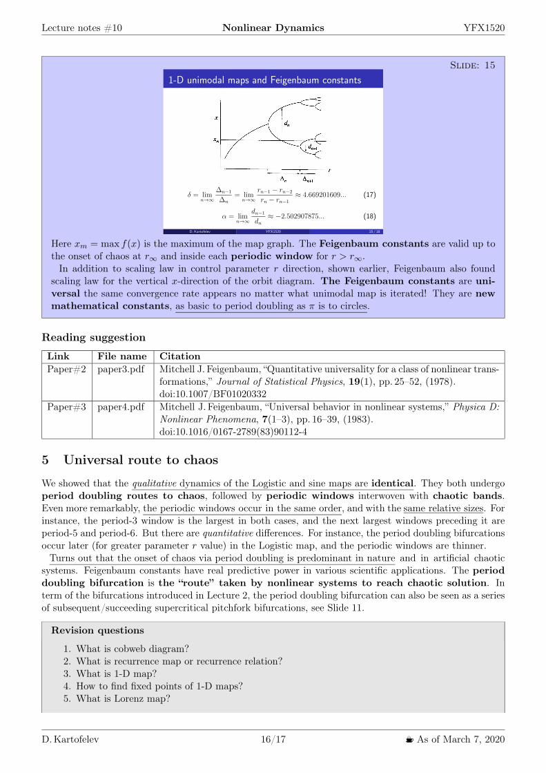
Lecture notes 10 Nonlinear Dynamics YFX1520
Slide 151-D unimodal maps and Feigenbaum constants
= limn1
n1
n= lim
n1
rn1 rn2
rn rn1 4669201609 (17)
crarr = limn1
dn1
dn 2502907875 (18)
DKartofelev YFX1520 15 18
Here xm = max f(x) is the maximum of the map graph The Feigenbaum constants are valid up tothe onset of chaos at rinfin and inside each periodic window for r gt rinfin
In addition to scaling law in control parameter r direction shown earlier Feigenbaum also foundscaling law for the vertical x-direction of the orbit diagram The Feigenbaum constants are uni-versal the same convergence rate appears no matter what unimodal map is iterated They are newmathematical constants as basic to period doubling as π is to circles
Reading suggestion
Link File name CitationPaper2 paper3pdf Mitchell J Feigenbaum ldquoQuantitative universality for a class of nonlinear trans-
formationsrdquo Journal of Statistical Physics 19(1) pp 25ndash52 (1978)doi101007BF01020332
Paper3 paper4pdf Mitchell J Feigenbaum ldquoUniversal behavior in nonlinear systemsrdquo Physica DNonlinear Phenomena 7(1ndash3) pp 16ndash39 (1983)doi1010160167-2789(83)90112-4
5 Universal route to chaos
We showed that the qualitative dynamics of the Logistic and sine maps are identical They both undergoperiod doubling routes to chaos followed by periodic windows interwoven with chaotic bandsEven more remarkably the periodic windows occur in the same order and with the same relative sizes Forinstance the period-3 window is the largest in both cases and the next largest windows preceding it areperiod-5 and period-6 But there are quantitative differences For instance the period doubling bifurcationsoccur later (for greater parameter r value) in the Logistic map and the periodic windows are thinner
Turns out that the onset of chaos via period doubling is predominant in nature and in artificial chaoticsystems Feigenbaum constants have real predictive power in various scientific applications The perioddoubling bifurcation is the ldquorouterdquo taken by nonlinear systems to reach chaotic solution Interm of the bifurcations introduced in Lecture 2 the period doubling bifurcation can also be seen as a seriesof subsequentsucceeding supercritical pitchfork bifurcations see Slide 11
Revision questions
1 What is cobweb diagram2 What is recurrence map or recurrence relation3 What is 1-D map4 How to find fixed points of 1-D maps5 What is Lorenz map
D Kartofelev 1617 1003211 As of March 7 2020
Lecture notes 10 Nonlinear Dynamics YFX1520
6 What is Logistic map7 What is sine map8 What is period doubling9 What is period doubling bifurcation
10 What is tangent bifurcation11 Do odd number periods (period-p orbits) exist in chaotic systems12 Do even number periods (period-p orbits) exist in chaotic systems13 Can maps produce transient chaos14 Can maps produce intermittency15 Can maps produce intermittent chaos16 What is orbit diagram (or Feigenbaum diagram)17 What are Feigenbaum constants
D Kartofelev 1717 1003211 As of March 7 2020