Lecture 1 - VectorsA Puzzle...

The sum starts at 0. Players alternate by choosing an integer from 1 to 10 and then adding it to the sum. The player

who gets to 100 wins. You go first. What is the winning strategy?

Solution

Choose 1 (and then respond to your opponents number x with 11 - x)

Introduction

Welcome to Ph 1a Section 5 (the coolest section of them all)!

TA’s Information

◼ Name: Tal Einav

◼ Website: http://www.its.caltech.edu/~teinav

◼ Office: Broad 155

◼ Office Hours: Tuesday 4:00-5:00pm

◼ Ask questions!

"The goal of teaching should not be to implant in the student’s mind every fact that the teacher knows now; but

rather to implant a way of thinking that will enable the student, in the future, to learn in one year what the teacher

learned in two years. Only in that way can we continue to advance from one generation to the next."

- A Backward Look to the Future, E. T. Jaynes

Vectors: The quest begins!

Vectors

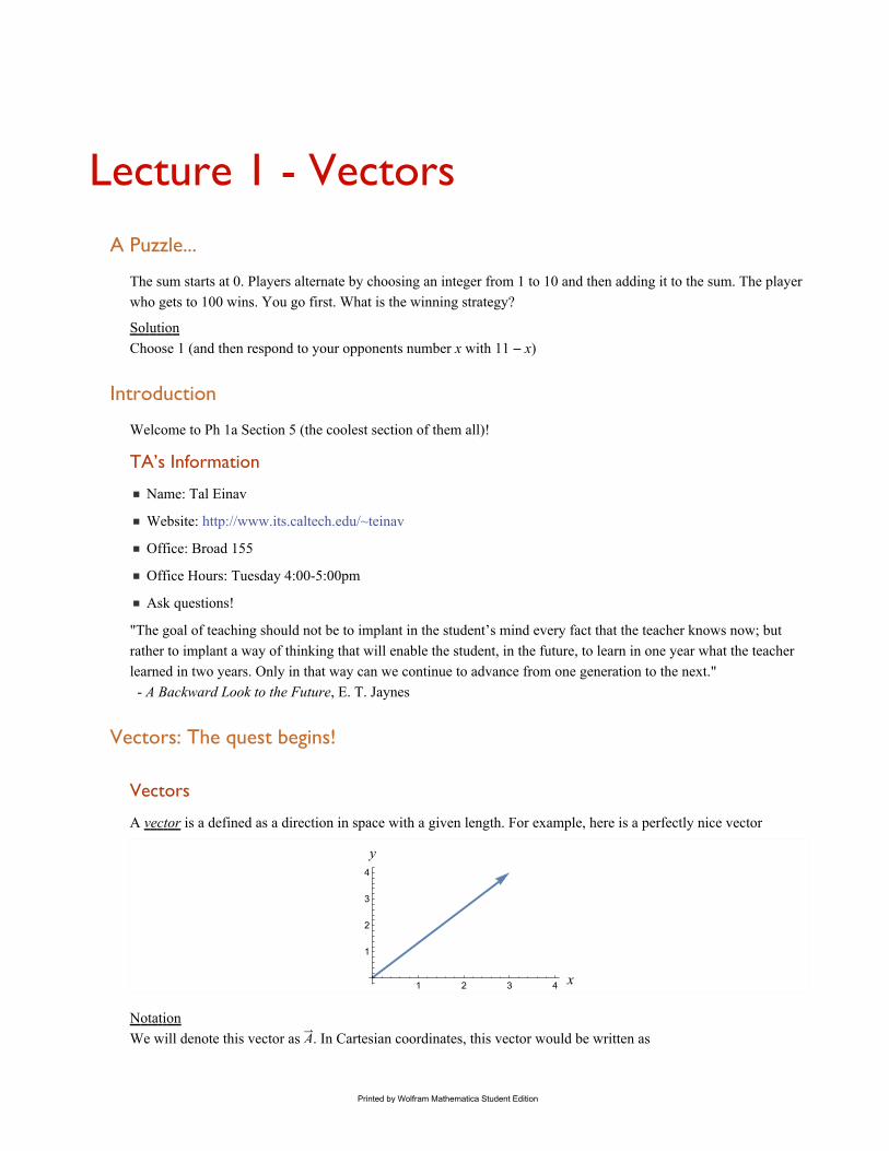
A vector is a defined as a direction in space with a given length. For example, here is a perfectly nice vector

1 2 3 4 x

1

2

3

4

y

Notation

We will denote this vector as A. In Cartesian coordinates, this vector would be written as

Printed by Wolfram Mathematica Student Edition

A = 3 x+ 4 y

(1)

where x and y represent the unit vectors in the x and y directions, respectively. If we were in 3D coordinates, z

would represent a unit vector in the z direction. Other common notations for the components include

A = (3, 4) (2)A = ⟨3, 4⟩ (3)

When using such notations, we implicitly assume Cartesian coordinates (and not, for example, polar coordinates).

2D Vectors

A generic 2D vector in Cartesian coordinates is

A = Ax x+ Ay y

(4)

The magnitude of the vector A equals Ax2 + Ay

2 and is denoted by A. The zero vector will be denoted by 0 and

represents a vector with 0 for each of its Cartesian coordinates. In polar coordinates, A would be written as

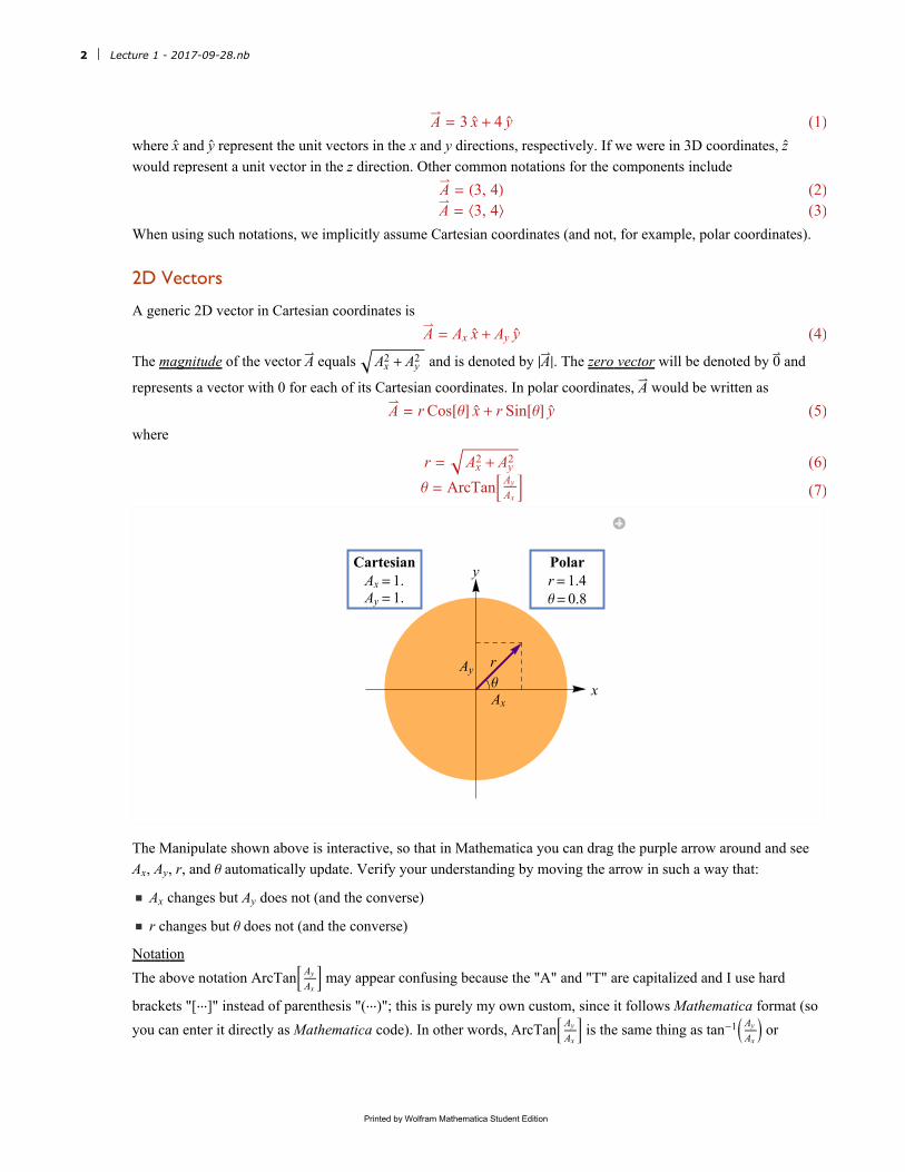
A = r Cos[θ] x+ r Sin[θ] y

(5)

where

r = Ax2 + Ay

2 (6)

θ = ArcTanAy

Ax (7)

x

y

θ

r

Ax

Ay

CartesianAx =1.Ay =1.

Polarr=1.4θ=0.8

The Manipulate shown above is interactive, so that in Mathematica you can drag the purple arrow around and see

Ax, Ay, r, and θ automatically update. Verify your understanding by moving the arrow in such a way that:

◼ Ax changes but Ay does not (and the converse)

◼ r changes but θ does not (and the converse)

Notation

The above notation ArcTanAy

Ax

may appear confusing because the "A" and "T" are capitalized and I use hard

brackets "[···]" instead of parenthesis "(···)"; this is purely my own custom, since it follows Mathematica format (so

you can enter it directly as Mathematica code). In other words, ArcTanAy

Ax

is the same thing as tan-1Ay

Ax

or

2 Lecture 1 - 2017-09-28.nb

Printed by Wolfram Mathematica Student Edition

arctanAy

Ax

. I will do this same capitalization and hard brackets format with any function: for example Cos[π] is

equivalent to cos(π).

Trig Review

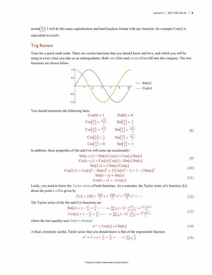
Time for a quick math aside. There are certain functions that you should know and love, and which you will be

using in every class you take as an undergraduate. Both sine (Sin) and cosine (Cos) fall into this category. The two

functions are shown below.

1 2 3 4 5 6

-1.0

-0.5

0.5

1.0

Sin[x]

Cos[x]

You should memorize the following facts:Cos[0] = 1 Sin[0] = 0

Cosπ

6 =

32

Sinπ

6 =

12

Cosπ

4 =

22

Sinπ

4 =

22

Cosπ

3 =

12

Sinπ

3 =

32

Cosπ

2 = 0 Sin

π

2 = 1

(8)

In addition, these properties of Sin and Cos will come up occasionally:

Sin[x+ y] = Sin[x] Cos[y] +Cos[x] Sin[y]Cos[x+ y] = Cos[x] Cos[y] - Sin[x] Sin[y]

(9)

Sin[2 x] = 2 Sin[x] Cos[x]Cos[2 x] = Cos[x]2 - Sin[x]2 = 2 Cos[x]2 - 1 = 1- 2 Sin[x]2

(10)

Sin[π - x] = Sin[x]Cos[π - x] = -Cos[x]

(11)

Lastly, you need to know the Taylor series of both functions. As a reminder, the Taylor series of a function f [x]

about the point x = 0 is given by

f [x] = f [0] + f '[0]1!

x+f ''[0]2!

x2 +f '''[0]

3!x3 + · · · (12)

The Taylor series of the Sin and Cos functions are

Sin[x] = x-x3

3!+

x5

5!- · · · = ∑j=0

∞ (-1) j x2 j+1

(2 j+1)!=

ⅇⅈ x-ⅇ-ⅈ x

2 ⅈ

Cos[x] = 1- x2

2!+

x4

4!- · · · = ∑j=0

∞ (-1) j x2 j

(2 j)!=

ⅇⅈ x+ⅇ-ⅈ x

2

(13)

where the last equality uses Euler’s formula

ⅇⅈ x = Cos[x] + ⅈ Sin[x] (14)

A final, extremely useful, Taylor series that you should know is that of the exponential function

ⅇx = 1+ x+x2

2!+

x3

3!+ · · · = ∑j=0

∞ xj

j! (15)

Lecture 1 - 2017-09-28.nb 3

Printed by Wolfram Mathematica Student Edition

3D Vectors

A generic 3D vector in Cartesian coordinates is

A = Ax x+ Ay y

+ Az z

(16)

which in spherical polar coordinates equals

A = r Sin[θ] Cos[ϕ] x+ r Sin[θ] Sin[ϕ] y

+ r Cos[θ] z

(17)

where ϕ ∈ [0, 2 π) is the polar angle and θ ∈ [0, π] is the azimuthal angle.

Unfortunately, as seen above, physicists take the horrible convention where θ is the polar angle in 2D radial

coordinates but ϕ is the polar angle in 3D spherical coordinates. Therefore, to regain polar coordinates from

spherical coordinates you must set θ = π

2 and then rename ϕ = θ. (Mathematicians, on the other hand, tend to

switch the definitions of θ and ϕ in spherical coordinates to avoid this issue!)

We can convert from Cartesian coordinates to spherical coordinates using

r = Ax2 + Ay

2 + Az2 (18)

ϕ = ArcTanAy

Ax (19)

θ = ArcTanAx

2+Ay2

1/2

Az = ArcCos

Az

Ax2+Ay

2+Az2

1/2 (20)

(I encourage you to verify that both of these expressions for θ are equal!)

The last 3D coordinate system worth mentioning is cylindrical coordinates. This system is rarely used in classical

mechanics and the book does not mention it, so we will skip it for now. However, you invited to consult

Wikipedia to refresh your memory on this system (this system will definitely be used next term in Electromag-

netism).

Including Cartesian coordinates, here is a pictorial summary of the four most important coordinate systems.

4 Lecture 1 - 2017-09-28.nb

Printed by Wolfram Mathematica Student Edition

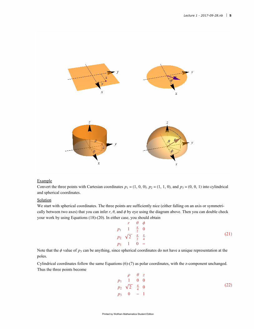
Example

Convert the three points with Cartesian coordinates p1 = (1, 0, 0), p2 = (1, 1, 0), and p3 = (0, 0, 1) into cylindrical

and spherical coordinates.

Solution

We start with spherical coordinates. The three points are sufficiently nice (either falling on an axis or symmetri-

cally between two axes) that you can infer r, θ, and ϕ by eye using the diagram above. Then you can double check

your work by using Equations (18)-(20). In either case, you should obtainr θ ϕ

p1 1 π

20

p2 2 π

2π

4

p3 1 0 -

(21)

Note that the ϕ value of p3 can be anything, since spherical coordinates do not have a unique representation at the

poles.

Cylindrical coordinates follow the same Equations (6)-(7) as polar coordinates, with the z-component unchanged.

Thus the three points becomeρ θ z

p1 1 0 0

p2 2 π

40

p3 0 - 1

(22)

Lecture 1 - 2017-09-28.nb 5

Printed by Wolfram Mathematica Student Edition

Note that the θ coordinate can be anything for p3, since cylindrical coordinates do not have a unique representation

on the z-axis. □

Integration

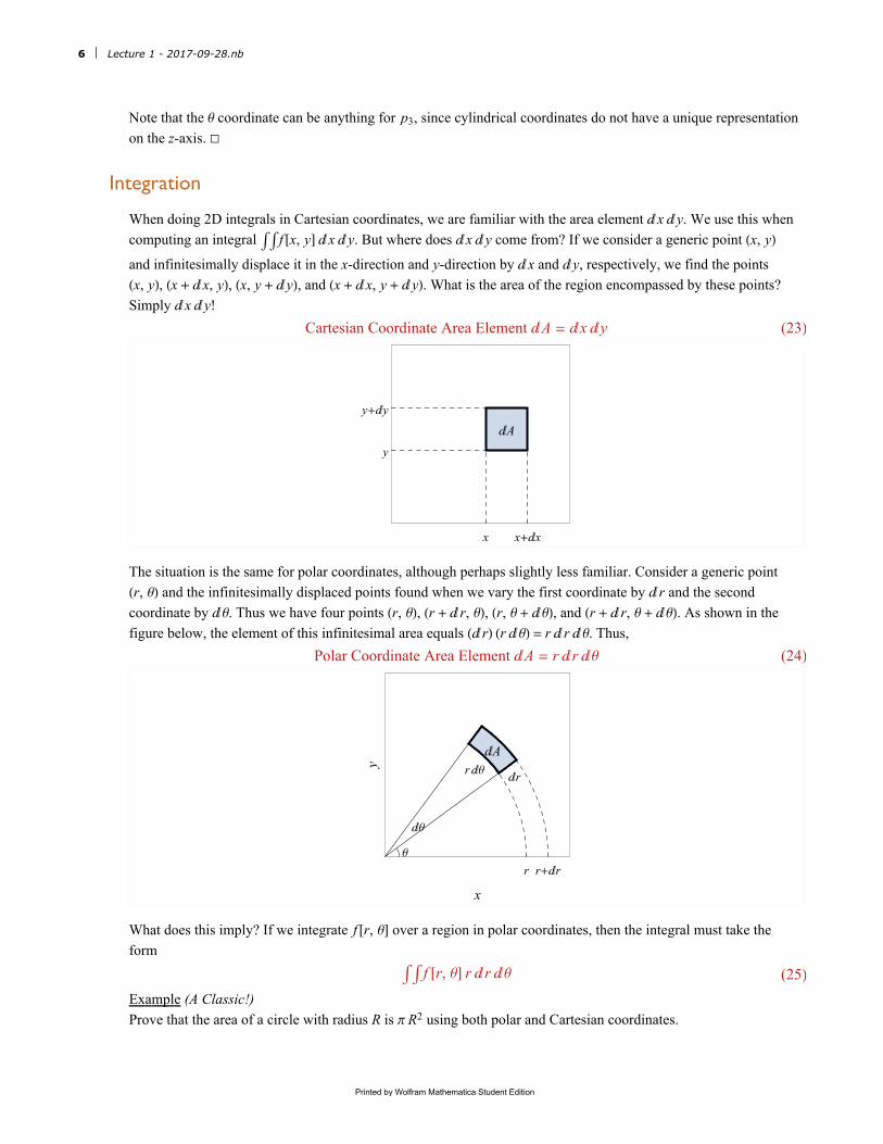
When doing 2D integrals in Cartesian coordinates, we are familiar with the area element ⅆ x ⅆ y. We use this when

computing an integral ∫ ∫ f [x, y] ⅆ x ⅆ y. But where does ⅆ x ⅆ y come from? If we consider a generic point (x, y)

and infinitesimally displace it in the x-direction and y-direction by ⅆ x and ⅆ y, respectively, we find the points

(x, y), (x + ⅆ x, y), (x, y + ⅆ y), and (x + ⅆ x, y + ⅆ y). What is the area of the region encompassed by these points?

Simply ⅆ x ⅆ y!

Cartesian Coordinate Area Element ⅆA = ⅆx ⅆy (23)

ⅆA

x x+ⅆx

y

y+ⅆy

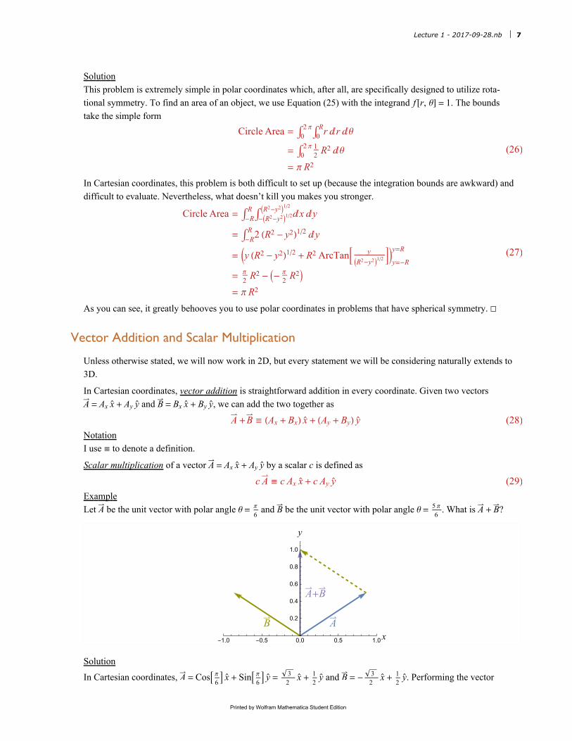
The situation is the same for polar coordinates, although perhaps slightly less familiar. Consider a generic point

(r, θ) and the infinitesimally displaced points found when we vary the first coordinate by ⅆ r and the second

coordinate by ⅆ θ. Thus we have four points (r, θ), (r + ⅆ r, θ), (r, θ + ⅆ θ), and (r + ⅆ r, θ + ⅆ θ). As shown in the

figure below, the element of this infinitesimal area equals (ⅆ r) (r ⅆ θ) = r ⅆ r ⅆ θ. Thus,

Polar Coordinate Area Element ⅆA = r ⅆr ⅆθ (24)

θ

ⅆθ

r ⅆθⅆr

ⅆA

r r+ⅆr

x

y

What does this imply? If we integrate f [r, θ] over a region in polar coordinates, then the integral must take the

form

∫ ∫ f [r, θ] r ⅆr ⅆθ (25)

Example (A Classic!)

Prove that the area of a circle with radius R is π R2 using both polar and Cartesian coordinates.

6 Lecture 1 - 2017-09-28.nb

Printed by Wolfram Mathematica Student Edition

Solution

This problem is extremely simple in polar coordinates which, after all, are specifically designed to utilize rota-

tional symmetry. To find an area of an object, we use Equation (25) with the integrand f [r, θ] = 1. The bounds

take the simple form

Circle Area = ∫02 π

∫0Rr ⅆr ⅆθ

= ∫02 π 1

2R2 ⅆθ

= π R2

(26)

In Cartesian coordinates, this problem is both difficult to set up (because the integration bounds are awkward) and

difficult to evaluate. Nevertheless, what doesn’t kill you makes you stronger.

Circle Area = ∫-R

R∫-R2-y2

1/2R2-y2

1/2

ⅆx ⅆy

= ∫-R

R 2 (R2 - y2)1/2 ⅆy

= y (R2 - y2)1/2 + R2 ArcTany

R2-y21/2

y=-R

y=R

=π

2R2 - -

π

2R2

= π R2

(27)

As you can see, it greatly behooves you to use polar coordinates in problems that have spherical symmetry. □

Vector Addition and Scalar Multiplication

Unless otherwise stated, we will now work in 2D, but every statement we will be considering naturally extends to

3D.

In Cartesian coordinates, vector addition is straightforward addition in every coordinate. Given two vectors

A = Ax x+ Ay y

and B = Bx x+ By y

, we can add the two together as

A +B ≡ (Ax + Bx) x+ (Ay + By) y

(28)

Notation

I use ≡ to denote a definition.

Scalar multiplication of a vector A = Ax x+ Ay y

by a scalar c is defined as

c A ≡ c Ax x+ c Ay y

(29)

Example

Let A be the unit vector with polar angle θ = π

6 and B be the unit vector with polar angle θ = 5 π

6. What is A + B?

AB

A+B

-1.0 -0.5 0.0 0.5 1.0 x

0.2

0.4

0.6

0.8

1.0

y

Solution

In Cartesian coordinates, A = Cosπ

6 x

+ Sin

π

6 y

=

32

x+

12

y and B = -

32

x+

12

y. Performing the vector

Lecture 1 - 2017-09-28.nb 7

Printed by Wolfram Mathematica Student Edition

addition yields A +B = y. Of course, the symmetry of the problem indicated that A +B must point in the y-direction

and have no x-component. □

Dot Product

Given two vectors A = Ax x+ Ay y

and B = Bx x+ By y

, we define the dot product of A and B as

A · B ≡ Ax Bx + Ay By (30)

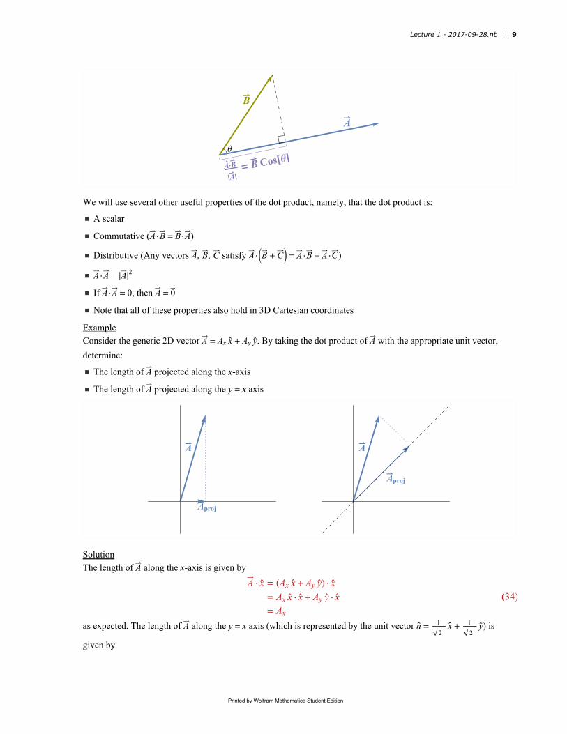
But a much better representation of the dot product (and the way you should visualize it in your mind) is using the

following theorem.

Theorem

Given two vectors A = Ax x+ Ay y

and B = Bx x+ By y

, the dot product of these two vectors equals

A · B = A B Cos[θ] (31)

θ

A

B

A·B

A

= BCos[θ]

Proof

We can write A and B in polar coordinates as (r1, θ1) and (r2, θ2), respectively. Then the dot product definition

gives

A · B = Ax Bx + Ay By

= r1 r2(Cos[θ1] Cos[θ2] + Sin[θ1] Sin[θ2])

= r1 r2 Cos[θ1 - θ2]

= A B Cos[θ]

(32)

where θ = θ1 - θ2 is the angle between A and B (recall that Cosine is an even function, so it does not matter if

θ1 ≤ θ2 or θ2 ≤ θ1). □

Properties of the Dot Product

Equation (31) is important! It immediately leads us to the most important way to think about the dot product:

The dot product of a vector A with any unit vector equals the component of A in the direction of that

unit vector.(33)

8 Lecture 1 - 2017-09-28.nb

Printed by Wolfram Mathematica Student Edition

θ

A

B

A·B

A

= BCos[θ]

We will use several other useful properties of the dot product, namely, that the dot product is:

◼ A scalar

◼ Commutative (A ·B = B ·A)

◼ Distributive (Any vectors A, B, C satisfy A ·B + C = A ·B + A ·C)

◼ A ·A = A2

◼ If A ·A = 0, then A = 0

◼ Note that all of these properties also hold in 3D Cartesian coordinates

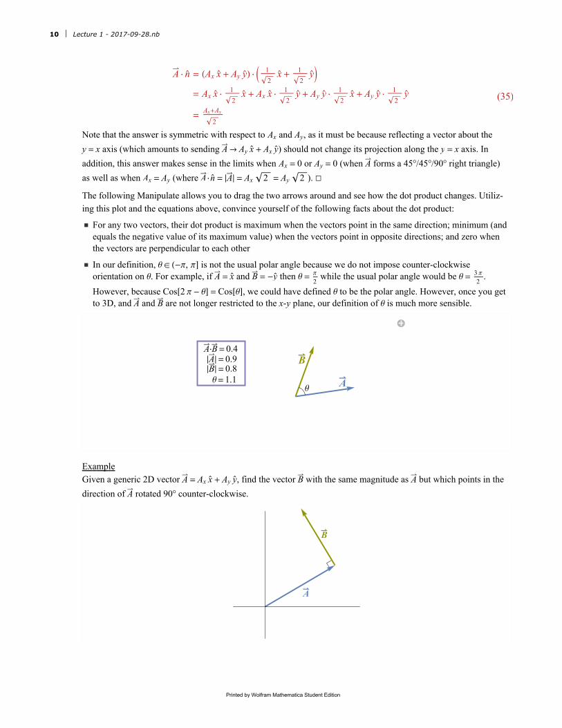
Example

Consider the generic 2D vector A = Ax x+ Ay y

. By taking the dot product of A with the appropriate unit vector,

determine:

◼ The length of A projected along the x-axis

◼ The length of A projected along the y = x axis

A

Aproj

A

Aproj

Solution

The length of A along the x-axis is given by

A · x= (Ax x

+ Ay y

) · x

= Ax x· x

+ Ay y

· x

= Ax

(34)

as expected. The length of A along the y = x axis (which is represented by the unit vector n = 1

2x+

1

2y) is

given by

Lecture 1 - 2017-09-28.nb 9

Printed by Wolfram Mathematica Student Edition

A · n= (Ax x

+ Ay y

) ·

1

2x+

1

2y

= Ax x·

1

2x+ Ax x

·

1

2y+ Ay y

·

1

2x+ Ay y

·

1

2y

=Ax+Ay

2

(35)

Note that the answer is symmetric with respect to Ax and Ay, as it must be because reflecting a vector about the

y = x axis (which amounts to sending A → Ay x+ Ax y

) should not change its projection along the y = x axis. In

addition, this answer makes sense in the limits when Ax = 0 or Ay = 0 (when A forms a 45°/45°/90° right triangle)

as well as when Ax = Ay (where A ·n= A = Ax 2 = Ay 2 ). □

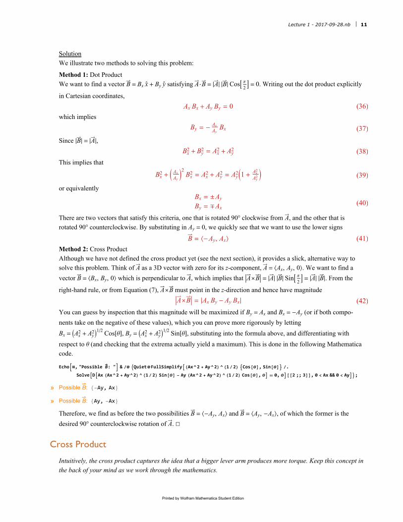
The following Manipulate allows you to drag the two arrows around and see how the dot product changes. Utiliz-

ing this plot and the equations above, convince yourself of the following facts about the dot product:

◼ For any two vectors, their dot product is maximum when the vectors point in the same direction; minimum (and equals the negative value of its maximum value) when the vectors point in opposite directions; and zero when the vectors are perpendicular to each other

◼ In our definition, θ ∈ (-π, π] is not the usual polar angle because we do not impose counter-clockwise orientation on θ. For example, if A = x

and B = -y then θ = π

2 while the usual polar angle would be θ = 3 π

2.

However, because Cos[2 π - θ] = Cos[θ], we could have defined θ to be the polar angle. However, once you get to 3D, and A and B are not longer restricted to the x-y plane, our definition of θ is much more sensible.

θA

B

A·B=0.4A=0.9B=0.8

θ=1.1

Example

Given a generic 2D vector A = Ax x+ Ay y

, find the vector B with the same magnitude as A but which points in the

direction of A rotated 90° counter-clockwise.

A

B

10 Lecture 1 - 2017-09-28.nb

Printed by Wolfram Mathematica Student Edition

Solution

We illustrate two methods to solving this problem:

Method 1: Dot Product

We want to find a vector B = Bx x+ By y

satisfying A ·B = A B Cosπ

2 = 0. Writing out the dot product explicitly

in Cartesian coordinates,

Ax Bx + Ay By = 0 (36)

which implies

By = -Ax

AyBx (37)

Since B = A,

Bx2 + By

2 = Ax2 + Ay

2 (38)

This implies that

Bx2 +

Ax

Ay2

Bx2 = Ax

2 + Ay2 = Ay

21+ Ax2

Ay2 (39)

or equivalentlyBx = ±Ay

By = ∓Ax(40)

There are two vectors that satisfy this criteria, one that is rotated 90° clockwise from A, and the other that is

rotated 90° counterclockwise. By substituting in Ay = 0, we quickly see that we want to use the lower signs

B = ⟨-Ay, Ax⟩ (41)

Method 2: Cross Product

Although we have not defined the cross product yet (see the next section), it provides a slick, alternative way to

solve this problem. Think of A as a 3D vector with zero for its z-component, A = ⟨Ax, Ay, 0⟩. We want to find a

vector B = ⟨Bx, By, 0⟩ which is perpendicular to A, which implies that A⨯B = A B Sinπ

2 = A B. From the

right-hand rule, or from Equation (7), A⨯B must point in the z-direction and hence have magnitude

A⨯B = Ax By - Ay Bx (42)

You can guess by inspection that this magnitude will be maximized if By = Ax and Bx = -Ay (or if both compo-

nents take on the negative of these values), which you can prove more rigorously by letting

Bx = Ax2 + Ay

21/2 Cos[θ], By = Ax

2 + Ay2

1/2 Sin[θ], substituting into the formula above, and differentiating with

respect to θ (and checking that the extrema actually yield a maximum). This is done in the following Mathematica

code.

Echo#, "Possible B: " & /@ Quiet@FullSimplify(Ax^2 + Ay^2)^(1/2) Cos[θ], Sin[θ] /.

SolveDAx (Ax^2 + Ay^2)^(1/2) Sin[θ] - Ay (Ax^2 + Ay^2)^(1/2) Cos[θ], θ ⩵ 0, θ[[2 ;; 3]], 0 < Ax && 0 < Ay;

» Possible B

: {-Ay, Ax}

» Possible B

: {Ay, -Ax}

Therefore, we find as before the two possibilities B = ⟨-Ay, Ax⟩ and B = ⟨Ay, -Ax⟩, of which the former is the

desired 90° counterclockwise rotation of A. □

Cross Product

Intuitively, the cross product captures the idea that a bigger lever arm produces more torque. Keep this concept in

the back of your mind as we work through the mathematics.

Lecture 1 - 2017-09-28.nb 11

Printed by Wolfram Mathematica Student Edition

of your through

(43)

In this section, we work in 3D Cartesian coordinates because the cross product is not defined in 2D.

Given two vectors A = Ax x+ Ay y

+ Az z

and B = Bx x+ By y

+ Bz z

, we define the cross product of A and B as

A⨯B ≡ (Ay Bz - Az By) x+ (Az Bx - Ax Bz) y

+ (Ax By - Ay Bx) z

(44)

A useful way to remember this formula is using the matrix determinant

A⨯B =

x

y

z

Ax Ay Az

Bx By Bz

(45)

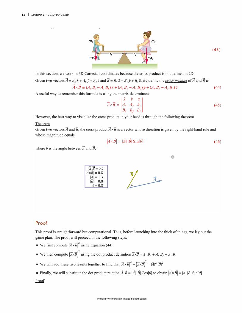
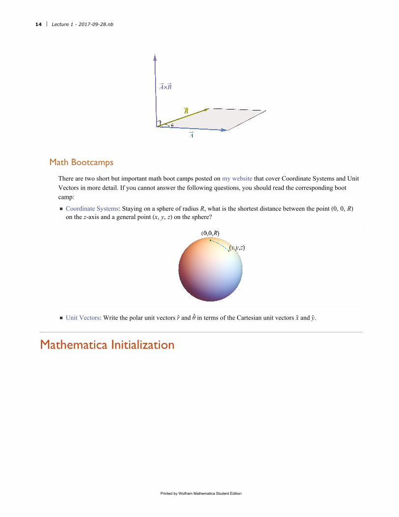
However, the best way to visualize the cross product in your head is through the following theorem.

Theorem

Given two vectors A and B, the cross product A⨯B is a vector whose direction is given by the right-hand rule and

whose magnitude equals

A⨯B = A B Sin[θ] (46)

where θ is the angle between A and B.

θ

A

B

A·B=0.7A⨯B=0.8

A=1.3B=0.8

θ=0.8

Proof

This proof is straightforward but computational. Thus, before launching into the thick of things, we lay out the

game plan. The proof will proceed in the following steps:

◼ We first compute A⨯B2 using Equation (44)

◼ We then compute A ·B2 using the dot product definition A ·B = Ax Bx + Ay By + Az Bz

◼ We will add these two results together to find that A ⨯B2+ A ·B

2= A

2B

2

◼ Finally, we will substitute the dot product relation A ·B = A B Cos[θ] to obtain A⨯B = A B Sin[θ]

Proof

12 Lecture 1 - 2017-09-28.nb

Printed by Wolfram Mathematica Student Edition

Using Equation (44), we compute

A⨯B2= (Ay Bz - Az By)

2 + (Az Bx - Ax Bz)2 + (Ax By - Ay Bx)

2

= Ax2(By

2 + Bz2) + Ay

2(Bx2 + Bz

2) + Az2(Bx

2 + By2)

-2 (Ax Ay Bx By + Ay Az By Bz + Ax Az Bx Bz)

(47)

We next expand A ·B2= (Ax Bx + Ay By + Az Bz)

2 to obtain

A · B2= Ax

2 Bx2 + Ay

2 By2 + Az

2 Bz2

+2 (Ax Ay Bx By + Ay Az By Bz + Ax Az Bx Bz)(48)

Note that the last terms in both A⨯B2 and A ·B

2 are equal and opposite, so that they will cancel when we add

both quantities,

A⨯B2+ A · B

2= Ax

2(Bx2 + By

2 + Bz2) + Ay

2(Bx2 + By

2 + Bz2) + Az

2(Bx2 + By

2 + Bz2)

= (Ax2 + Ay

2 + Az2) (Bx

2 + By2 + Bz

2)

= A2

B2

(49)

Using the dot product relation A ·B = A B Cos[θ], we can rewrite this last formula as

A⨯B2= A

2B

2- A · B

2

= A2

B2- A

2B

2 Cos[θ]2

= A2

B2 Sin[θ]2

(50)

which completes the proof of Equation (46). All that remains is to show that the vector A ⨯B defined by Equation

(44) always follows the right-hand rule. It might seem trivial, but proving this rigorously is surprisingly difficult,

and I leave this fun problem as an exercise for the reader! □

Cross Product Properties

Equations (44) and (46) give us the keys to the cross product kingdom. From them, it is straightforward to extract

that the cross product is:

◼ A vector

◼ Anti-commutative (A⨯B = -B⨯A)

◼ Not associative (Given vectors A, B, C, it is not true that A⨯B⨯C = A⨯B⨯C. Counter-example:

A = x, B = x

, C = y)

◼ Distributive over addition (Any vectors A, B, C satisfy A⨯B + C = A⨯B + A⨯C)

◼ For any vectors A, B and scalar c, c A⨯B = c A⨯B = A⨯c B

◼ For any vector A, A⨯A = 0

◼ Given two vectors A and B, the cross product A⨯B is orthogonal to both A and B.

Lecture 1 - 2017-09-28.nb 13

Printed by Wolfram Mathematica Student Edition

Math Bootcamps

There are two short but important math boot camps posted on my website that cover Coordinate Systems and Unit

Vectors in more detail. If you cannot answer the following questions, you should read the corresponding boot

camp:

◼ Coordinate Systems: Staying on a sphere of radius R, what is the shortest distance between the point (0, 0, R) on the z-axis and a general point (x, y, z) on the sphere?

◼ Unit Vectors: Write the polar unit vectors r and θ in terms of the Cartesian unit vectors x and y.

Mathematica Initialization

14 Lecture 1 - 2017-09-28.nb

Printed by Wolfram Mathematica Student Edition