Lecture 1 Stochastic Optimization: IntroductionUday V. Shanbhag Lecture 1 Unconstrained optimization Unconstrained minimize x2Rn f(x) Xis de ned as X,Rn Examples: f(x) = x3 3x2. Important

Lecture 1

Stochastic Optimization: Introduction

January 8, 2018

Uday V. Shanbhag Lecture 1

Optimization

• Concerned with mininmization/maximization of mathematical functions

• Often subject to constraints

• Euler (1707-1783): Nothing at all takes place in the universe in which

some rule of the maximum or minimum does not apply.

• Important tool in the analysis/design/control/simulation of physical,

economic, chemical and biological systems

• Model → apply algorithm → check solution

Stochastic Optimization 1


Unconstrained optimization

Unconstrained minimizex∈Rn

f(x)

• X is defined as X , Rn

• Examples: f(x) = x3 − 3x2.

• Important application: Data fitting and regression



Unconstrained optimization: An example

Given a data set yi, xi1, . . . , xipnp=1 (n records, with the dependent

variable yi and independent variable xi1, . . . , xip).

The linear regression model assumes that the relationship between the

dependent variable y and the independent variables xi is linear. This

relation is captured as follows:

yi = xi0 +p∑

j=1

βpxip + εi, i = 1, . . . , n

where εi denotes a random variable. More compactly, we may state this as

follows:

y = Xβ + ε, where y ,

y1...

yn

, X ,xT1•

...

xTn•

.



Then the least-squares estimator β is defined as follows:

β = argminβ‖Xβ − y‖2.



Convex optimization

Convex minimizex∈Rn

f(x)

subject to x ∈ X,

where X is a convex set and f is a convex function.

Definition 1 (Convexity of sets and functions)

• A set X ⊆ Rn is a convex set if x1, x2 ∈ X then (λx1 + (1−λ)x2) ∈ Xfor all λ ∈ [0,1].

• A function f is said to be convex if

f(λx1 + (1− λ)x2) ≤ λf(x1) + (1− λ)f(x2), ∀λ ∈ [0,1].



• A function f is said to be strictly convex if

f(λx1 + (1− λ)x2) < λf(x1) + (1− λ)f(x2), ∀λ ∈ [0,1].

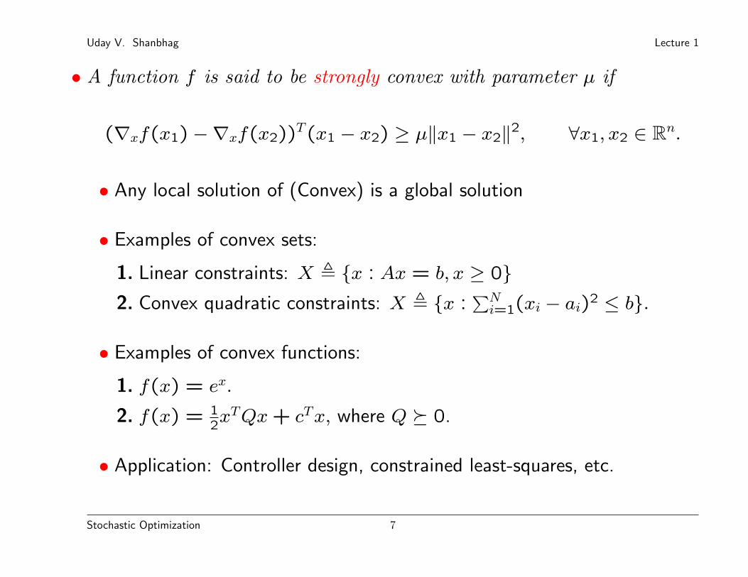
• A function f is said to be strongly convex with parameter µ if

f(λx1+(1−λ)x2) ≤ λf(x1)+(1−λ)f(x2)−12µλ(1−λ)‖x1−x2‖2, ∀λ ∈ [0,1].

Note that in the above definition f does not need to be differentiable.

Definition 2 (Convexity of differentiable functions) Consider a differ-

entiable function f : Rn → R.

• A function f is said to be convex if

f(x2) ≥ f(x1) +∇xf(x1)T(x2 − x1), ∀x1, x2 ∈ Rn.



• A function f is said to be strongly convex with parameter µ if

(∇xf(x1)−∇xf(x2))T(x1 − x2) ≥ µ‖x1 − x2‖2, ∀x1, x2 ∈ Rn.

• Any local solution of (Convex) is a global solution

• Examples of convex sets:

1. Linear constraints: X , x : Ax = b, x ≥ 02. Convex quadratic constraints: X , x :

∑Ni=1(xi − ai)2 ≤ b.

• Examples of convex functions:

1. f(x) = ex.

2. f(x) = 12xTQx+ cTx, where Q 0.

• Application: Controller design, constrained least-squares, etc.



Nonlinear program

NLP minimizex∈X

f(x)

• f : Objective function is a possibly nonconvex function

• x ∈ Rn: Decision variables

• X ⊆ Rn is a possibly nonconvex set

• f : X → R

• Applications: Nonlinear regression, process control in chemical engineer-

ing, etc.:



Discrete optimization

Discrete minimizex∈Rn

f(x)

subject to x ∈ Z.

• Z is a finite set implying that x can take on discrete values

• e.g. x ∈ 0,1.

• Sometimes x1 ∈ R, x2 ∈ 0,1; the resulting problem is called a

mixed-integer problem

• Applications: facility location problems, unit commitment problems



Convex optimization – relevance in this course

• Stochastic optimization captures a broad class of problems, including

convex, nonconvex (time permitting), and discrete optimization problems

(not considered here).

• In this course, we focus on the following:

• Convex stochastic optimization problems (including stochastic pro-

grams with recourse)

•Monotone stochastic variational inequality problems (subsumes stochas-

tic convex optimization and captures stochastic Nash games, stochas-

tic contact problems, stochastic traffic equilibrium problems)

• Robust optimization problems

• Applications: Statistical learning problems

• Convexity is crucial and will be leveraged extensively during the course!!



Problems complicated by uncertainty

• In the aforementioned (deterministic) problems, parameters are known

with certainty. Specifically, given a function f(x; ξ), we consider two

possibilities:

• ξ is a random variable. Our focus is then on solving the following:

minx∈X

E[f(x, ξ)] (Stoch-Opt)

• ξ is unavailable and instead we have that ξ ∈ U (where U is an

uncertainty set). A problem of interest is then:

minx∈X

maxξ∈U

f(x, ξ) (Robust-Opt)



•We motivate this line of questioning by considering the classical newsven-

dor problem



A short detour – Probability Spaces

• Throughout this course, we will be utilizing the notion of a probability

space (Ω,F ,P).

• This mathematical construct captures processes (either real or synthetic)

that are characterized by randomness.

• This space is constructed for a particular such process and on every

occasion this process is examined, both the set of outcomes and the

associated probabilities are the same.

• The sample-space Ω is a nonempty set that denotes the set of

outcomes. This represents a single execution of the experiment.

• The σ-algebra F denotes the set of events where each event is a set

containing zero or more outcomes.



• The assigmnent of probabilities to the events is captured by P.

• Once the space (Ω,F ,P) is established, then nature selects an outcome

ω from Ω. As a consequence, all events that contain ω as one of its

outcomes are said to have occurred.

• If nature selects outcomes infinitely often, then the relative frequencies

of occurrence of a particular event corresponds with the value specified

by the probability measure P.



• Properties of F :

• Ω ∈ F• F closed under complementation: A ∈ F =⇒ (Ω\A) ∈ F .

• F is closed under countable unions Ai ∈ F for i = 1,2 . . . , implies

that (⋃∞i=1Ai) ∈ F .

• Properties of P. The probability measure P : F → [0,1] such that P is

• P is countably additive: If Ai∞i=1 ∈ F denotes a countable col-

lection of pairwise disjoint sets (Ai ∩ Aj = ∅ for i 6= j), then

P(∪∞i=1Ai) =∑∞i=1 P(Ai).

• The measure of the sample-space is one or P(Ω) = 1.



A short detour – Probability Spaces: II

• Example 1. Single coin toss

• Ω , H,T.• The σ−algebra F contains 22 = 4 events

F , , H, T, H,T .

• Furthermore, P() = 0,P(H) = 0.5, P(T) = 0.5, and

P(H,T) = 1.

• Example 2. Double coin toss

• Ω , HH,HT, TH, TT.



• The σ−algebra F contains 24 = 16 events

F , , HH, TT, HT, TH,HH,TT, HH,HT, HH,THHT, TT, HT, TH, TH, TT,HH,HT, TH, HH,HT, TT, HH,TH, TT, HT, TH, TTHH,TH,HT,HH .

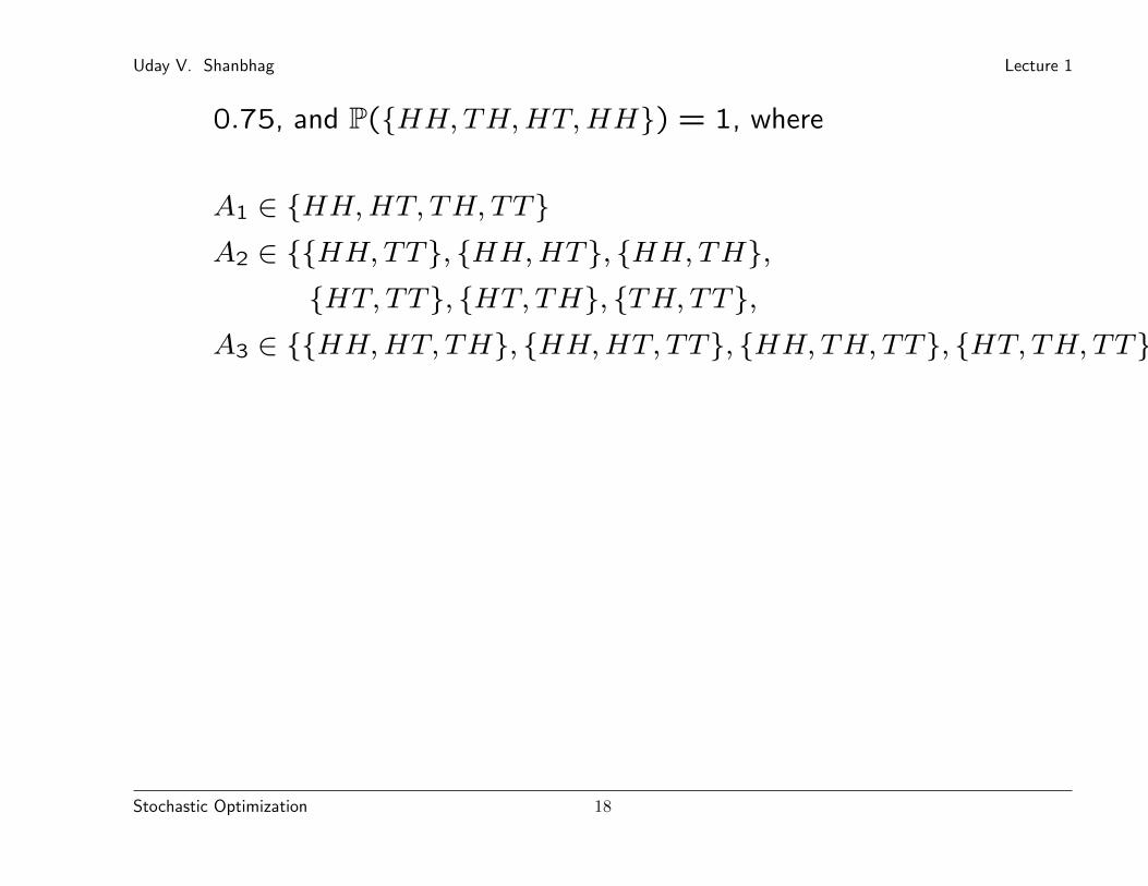
• Furthermore, P() = 0,P(A1) = 0.25, P(A2) = 0.5, P(A3) =



0.75, and P(HH,TH,HT,HH) = 1, where

A1 ∈ HH,HT, TH, TTA2 ∈ HH,TT, HH,HT, HH,TH,

HT, TT, HT, TH, TH, TT,A3 ∈ HH,HT, TH, HH,HT, TT, HH,TH, TT, HT, TH, TT ,



Random variables

• Given a probability space (Ω,F ,P), a random variable represents a

function on a sample-space with measurable values.

• Specifically, X is a random variable defined as X : Ω→ E, where E

is a measurable space.

• Consequently, P(X ∈ S) = P(ω ∈ Ω | X(ω) ∈ S).

• Example: Coin-tossing. Define X(ω) as follows:

X(ω) =

100, ω = H

−100, ω = T.



Example: The Newsvendor Problem

• Suppose a company has to decide its order quantity x, given a

demand d

• The cost is given by

f(x, d) , cx+ b[d− x]+︸︷︷︸back-order cost

+h[x− d]+︸︷︷︸holding cost

,

where b is back-order penalty and h is holding cost

• In such an instance, the firm will solve the problem:

minx≥0

f(x).



The Newsvendor Problem

• More specifically, suppose, demand is a random variable, defined as

dω , d(ω) where d : Ω→ R+ is a random variable, Ω is the sample

space

• Furthermore, suppose (Ω,F ,P) denotes the associated probability

space where P denotes the probability distribution function

• Then the (random) cost associated with demand dω is given by

f(x;ω) , cx+ b[dω − x]+︸︷︷︸back-order cost

+h[x− dω]+︸︷︷︸holding cost

,

•We assume for the present that P is known; then, the firm may



minimize its expected costs (averaged) given by

minx≥0

E[f(x;ω)],

where E[•] is the expectation with respect to P



The Newsvendor Problem

• This is an instance of a two-stage problem with recourse

First-stage decision: Order quantity x

Second-stage ω−specific recourse decisions: yω = [dω − x]+ and

zω = [x− dω]+.

• Recourse decisions can be taken upon revelation of uncertainty; first-

stage decisions have to be taken prior to this revelation



A Scenario-based Approach

• In practice, analytical solutions of this problem are complicated by

the presence of an expectation (integral)

• One avenue: a scenario-based approach requires obtaining K samples

from Ω, denoted by d(ω1), . . . , d(ωK) or d1, . . . , dK.

• The recourse-based problem is then given by

minimizeK∑k=1

pkf(x;ωk)

subject to x ≥ 0.



• Note that

f(x;ω) = cx+ b[dω − x]+ + h[x− dω]+

= max ((c− b)x+ bdω, (c+ h)x− hdω) .

minimizex,v1,...,vK

K∑k=1

pkvk

subject to

vk ≥ (c− b)x+ bdk, k = 1, . . . ,K

vk ≥ (c+ h)x− hdk, k = 1, . . . ,K

x ≥ 0

• This is a linear program with one possible challenge; as K grows, it

becomes increasingly difficult to solve directly



A two-stage linear program

• Consider the newsvendor problem again. It can be written as follows:

minimize cx+ E[Q(x;ω)]

subject to x ≥ 0.

where Q(x;ω) is the optimal value of the following recourse problem:

Q(x;ω) minimize [byω + hzω]

subject to

yω ≥ dω − x,zω ≥ x− dω,

yω, zω ≥ 0.



• The problem Q(x;ω) represents the cost of responding to the un-

certainty captured by realization ω and given the first-stage decision

x

• This motivates a canonical form for the two-stage stochastic linear

program:

minimize cTx+ E[Q(x; ξ)]

subject toAx = b

x ≥ 0.

where Q(x; ξ) is the optimal value of the following second-stage



recourse problem:

Q(x; ξ) minimize qTyξ

subject toTx+Wyξ = h

yξ ≥ 0,

and ξ := (q, T,W, h) represents the data of the second-stage problem

•We define Q(x), the cost of recourse, as follows:

Q(x) , E[Q(x;ω)].



A general model for stochastic optimization

A general model for stochastic optimization problems is given by the

following. Given a random variable ξ : Ω → Rd and a function

f : X × Rd → R, then the stochastic optimization problem requires an

x such that

Stoch-opt minimizex

E[f(x, ξ)]

subject to x ∈ X.

This model includes the case where f(x, ξ) = cTx + Q(x, ξ) as a

special case.



Analysis of two-stage stochastic programming

1. Properties of Q(x; ξ) (polyhedral, convex, etc.)

2. Expected recourse costs Q(x)

• Discrete distributions

• General distributions (convexity, continuity, Lipschitz continuity

etc.)

3. Optimality conditions

4. Extensions to convex regimes

5. Nonanticipativity

6. Value of perfect information



Decomposition methods for two-stage stochastic

programming

1. Cutting-plane methods

2. Extensions to convex nonlinear regimes

3. Dual decomposition methods



Monte-Carlo Sampling methods for convex stochastic

optimization

1. Stochastic decomposition schemes for two-stage stochastic linear

programs with general distributions

2. Sample-average approximation methods

• Consistency of estimators

• Convergence rates

3. Stochastic approximation methods

• Almost-sure convergence of iterates

• Non-asymptotic rates of convergence



Robust optimization problems

• Stochastic optimization relies on the availability of a distribution

function. In many settings, this is not available; instead, we have

access to a set for the uncertain parameter

• In such instance, one avenue lies in solving a robust optimization

problem

• Consider a linear optimization problem:

minx

cTx : Ax ≥ b, x ≥ 0

.

• The uncertain linear optimization problem is given by

minx

cTx : Ax ≥ b, x ≥ 0

(c,b,A)∈U



where U denotes the uncertainty set associated with the data.

• The robust counterpart of this problem is given by

minx

c(x) = sup

(c,b,A)∈U

cTx : Ax ≥ b, x ≥ 0, ∀(c, b, A) ∈ U

.

• This is effectively a problem in which the robust value of the objective

is minimized over all robust feasible solutions; a robust feasible

solution is defined as an x such that

Ax ≥ b, x ≥ 0, ∀(A, b) ∈ U .

• It can be seen that feasibility requirements lead to a semi-infinite

optimization problem; in other words, there is an infinite number

of constraints of the form Ax ≥ b, one for every (A, b) ∈ U . In



addition, the objective is of a min-max form, leading to a challenging

optimization problem

• Under some conditions on the uncertainty set, the robust optimization

problem can be recast as a convex optimization problem and is deemed

to be tractable. The first part of our study in robust optimization

will analyze the development of tractable robust counterparts for a

diverse set of uncertainty sets.

• In the second part of this topic, we will examine how chance con-

straints and their amobiguous variants can be captured via a tractable

problem.



Stochastic variational inequality problems

• Consider the convex optimization problem given by

minx∈X

f(x), (Opt)

where f : X → R is a continuously differentiable function and X is

a closed and convex set.

• Then x is a solution to (Opt) if and only if x is a solution to a

variational inequality problem, denoted by VI(X,∇xf). It may be

recalled that VI(X,F ) requires an x ∈ X such that

(y − x)TF (x) ≥ 0, ∀y ∈ X.



• Consider the stochastic generalization of (Opt) given by

minx∈X

E[f(x, ξ)], (SOpt)

where f : X × Rd → R is a convex function and E[.] denotes the

ecpectation with respect to a probability distribution P.

• The necessary and sufficienty conditions of optimality of this problem

are given by VI(X,F ) where F (x) , E[∇xf(x, ξ)].

• Variational inequality problems can capture the equilibrium conditions

of optimization problems and convex Nash games. Additionally, they

emerge in modeling a variety of problems including traffic equilibrium

problems, contact problems (in structural design), pricing of American

options, etc.

• Unfortunately, approaches for stochastic convex optimization cannot

be directly expected to function on variational inequality problems.



Instead, we extend stochastic approximation schemes to accommo-

date monotone stochastic variational inequality problems. Recall that

a map F is monotone over X if for all x, y ∈ X, we have that

(y − x)T(F (y)− F (x)) ≥ 0.


Documents

Lecture 1 Stochastic Optimization: IntroductionUday V. Shanbhag Lecture 1 Unconstrained optimization Unconstrained minimize x2Rn f(x) Xis de ned as X,Rn Examples: f(x) = x3 3x2. Important