Return to Main

Objectives

Physiology: Saggital View Saggital X-ray Vocal Cords Transduction Spectrogram

Acoustics: Acoustic Theory Wave Propagation Helium Speech

On-Line Resources: Spectrograms Acoustics and Speech Sound Waves in Tubes Tube Models Helium Speech

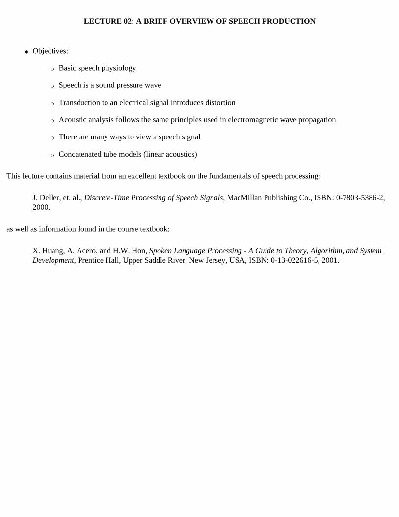
LECTURE 02: A BRIEF OVERVIEW OF SPEECH PRODUCTION

● Objectives:

❍ Basic speech physiology

❍ Speech is a sound pressure wave

❍ Transduction to an electrical signal introduces distortion

❍ Acoustic analysis follows the same principles used in electromagnetic wave propagation

❍ There are many ways to view a speech signal

❍ Concatenated tube models (linear acoustics)

This lecture contains material from an excellent textbook on the fundamentals of speech processing:

J. Deller, et. al., Discrete-Time Processing of Speech Signals, MacMillan Publishing Co., ISBN: 0-7803-5386-2, 2000.

as well as information found in the course textbook:

X. Huang, A. Acero, and H.W. Hon, Spoken Language Processing - A Guide to Theory, Algorithm, and System Development, Prentice Hall, Upper Saddle River, New Jersey, USA, ISBN: 0-13-022616-5, 2001.

Return to Main

Introduction:

01: Organization (html, pdf)

Speech Signals:

02: Production (html, pdf)

03: Digital Models (html, pdf)

04: Perception (html, pdf)

05: Masking (html, pdf)

06: Phonetics and Phonology (html, pdf)

07: Syntax and Semantics (html, pdf)

Signal Processing:

08: Sampling (html, pdf)

09: Resampling (html, pdf)

10: Acoustic Transducers (html, pdf)

11: Temporal Analysis (html, pdf)

12: Frequency Domain Analysis (html, pdf)

13: Cepstral Analysis (html, pdf)

14: Exam No. 1 (html, pdf)

15: Linear Prediction (html, pdf)

16: LP-Based Representations (html, pdf)

Parameterization:

17: Differentiation (html, pdf)

18: Principal Components (html, pdf)

ECE 8463: FUNDAMENTALS OF SPEECH RECOGNITION

Professor Joseph PiconeDepartment of Electrical and Computer Engineering

Mississippi State University

email: picone@isip.msstate.eduphone/fax: 601-325-3149; office: 413 Simrall

URL: http://www.isip.msstate.edu/resources/courses/ece_8463

Modern speech understanding systems merge interdisciplinary technologies from Signal Processing, Pattern Recognition, Natural Language, and Linguistics into a unified statistical framework. These systems, which have applications in a wide range of signal processing problems, represent a revolution in Digital Signal Processing (DSP). Once a field dominated by vector-oriented processors and linear algebra-based mathematics, the current generation of DSP-based systems rely on sophisticated statistical models implemented using a complex software paradigm. Such systems are now capable of understanding continuous speech input for vocabularies of hundreds of thousands of words in operational environments.

In this course, we will explore the core components of modern statistically-based speech recognition systems. We will view speech recognition problem in terms of three tasks: signal modeling, network searching, and language understanding. We will conclude our discussion with an overview of state-of-the-art systems, and a review of available resources to support further research and technology development.

Tar files containing a compilation of all the notes are available. However, these files are large and will require a substantial amount of time to download. A tar file of the html version of the notes is available here. These were generated using wget:

wget -np -k -m http://www.isip.msstate.edu/publications/courses/ece_8463/lectures/current

A pdf file containing the entire set of lecture notes is available here. These were generated using Adobe Acrobat.

Questions or comments about the material presented here can be directed to help@isip.msstate.edu.

19: Linear Discriminant Analysis (html, pdf)

LECTURE 02: A BRIEF OVERVIEW OF SPEECH PRODUCTION

● Objectives:

❍ Basic speech physiology

❍ Speech is a sound pressure wave

❍ Transduction to an electrical signal introduces distortion

❍ Acoustic analysis follows the same principles used in electromagnetic wave propagation

❍ There are many ways to view a speech signal

❍ Concatenated tube models (linear acoustics)

This lecture contains material from an excellent textbook on the fundamentals of speech processing:

J. Deller, et. al., Discrete-Time Processing of Speech Signals, MacMillan Publishing Co., ISBN: 0-7803-5386-2, 2000.

as well as information found in the course textbook:

X. Huang, A. Acero, and H.W. Hon, Spoken Language Processing - A Guide to Theory, Algorithm, and System Development, Prentice Hall, Upper Saddle River, New Jersey, USA, ISBN: 0-13-022616-5, 2001.

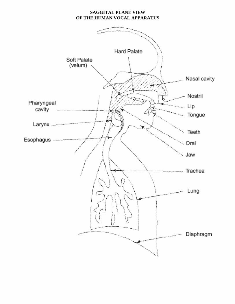
SAGGITAL PLANE VIEWOF THE HUMAN VOCAL APPARATUS

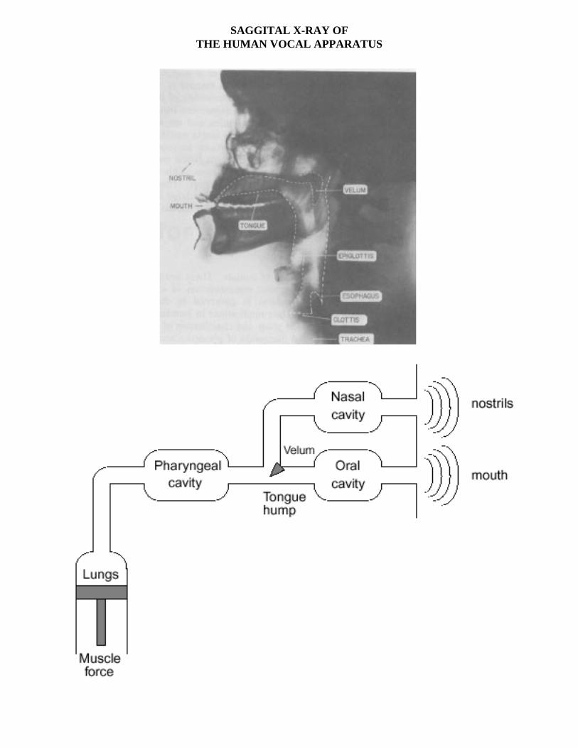
SAGGITAL X-RAY OFTHE HUMAN VOCAL APPARATUS

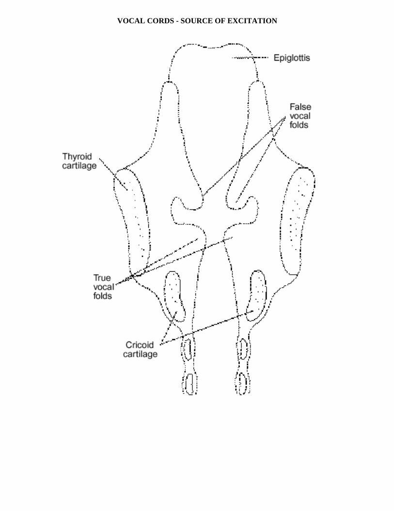
VOCAL CORDS - SOURCE OF EXCITATION

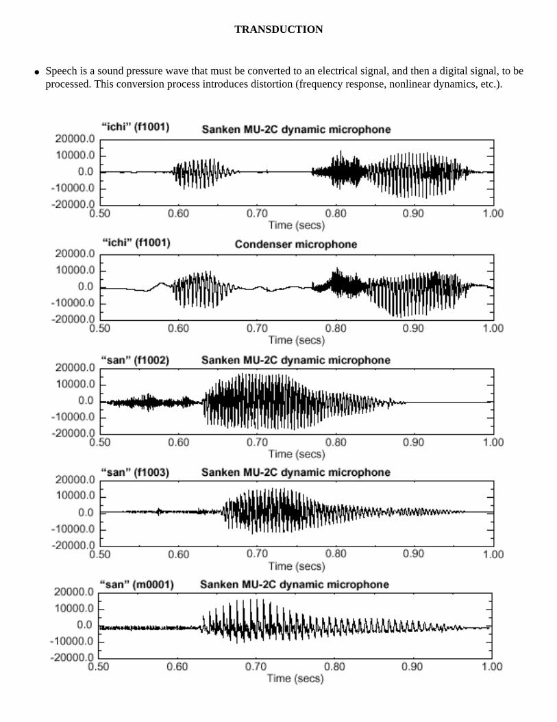
TRANSDUCTION

● Speech is a sound pressure wave that must be converted to an electrical signal, and then a digital signal, to be processed. This conversion process introduces distortion (frequency response, nonlinear dynamics, etc.).

WHAT DOES A SPEECH SIGNAL LOOK LIKE?

● We often prefer to view a spectrogram using a color visualization in which spectral log magnitude is mapped to "temperature" (the color that emanates from a steel bar when it is heated):

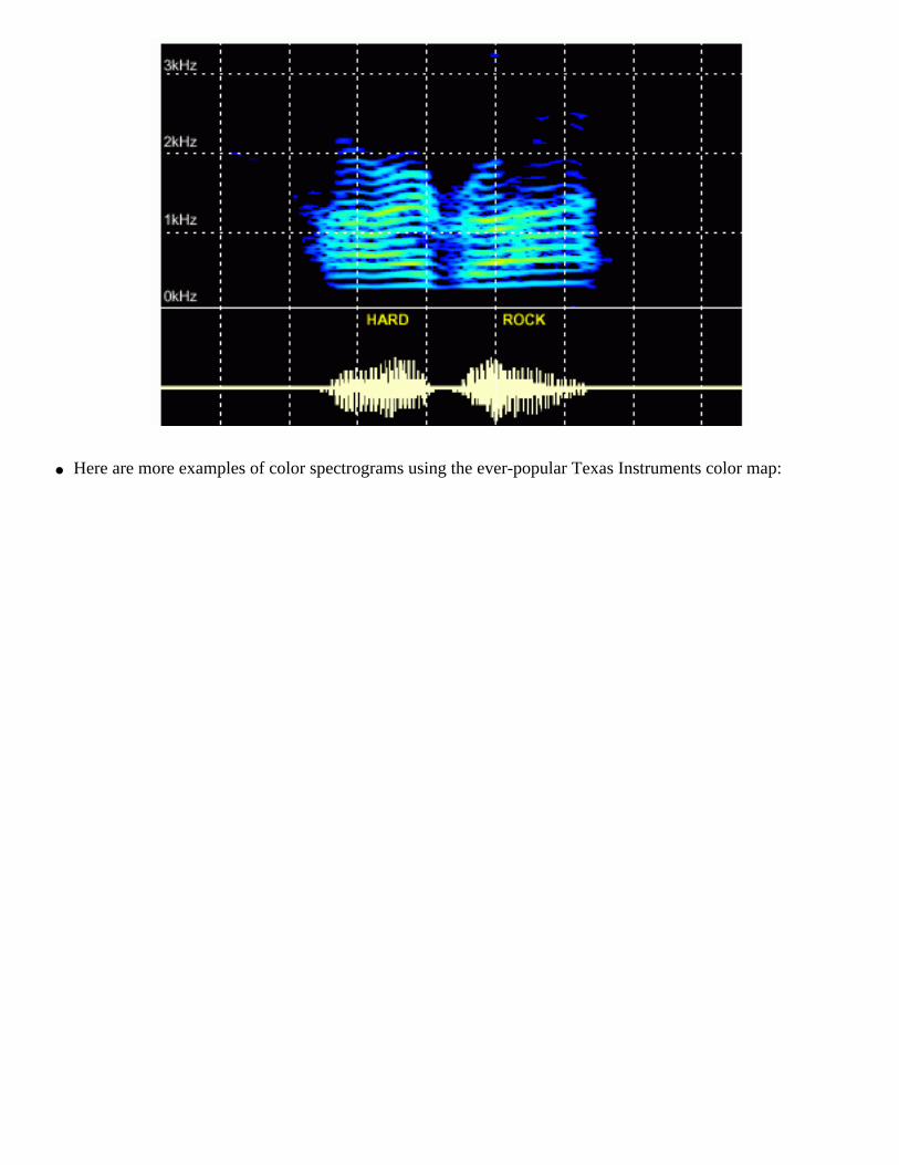
● Here are more examples of color spectrograms using the ever-popular Texas Instruments color map:

SOUND PROPAGATION - LINEAR ACOUSTICS

A detailed acoustic theory must consider the effects of the following:

● Time variation of the vocal tract shape

● Losses due to heat conduction and viscous friction at the vocal tract walls

● Softness of the vocal tract walls

● Radiation of sound at the lips

● Nasal coupling

● Excitation of sound in the vocal tract

● Let us consider a simple case of a lossless tube:

WAVE PROPAGATION

HELIUM SPEECH:RELATIONSHIP BETWEEN FREQUENCY AND DENSITY

● Deep-sea diving to depths exceeding about 140 feet of sea water requires the use of heliox (a mixture of helium and oxygen) as a breathing gas, rather than compressed air.

● Heliox eliminates the danger of nitrogen narcosis and reduces the risk of decompression sickness which would otherwise be present.

● Heliox presents another risk. The diver's speech is rendered unintelligible because the higher velocity of sound in the diver's vocal tract shifts the frequency components of the diver's speech to much higher frequencies - an effect that has been likened to the "Donald Duck" voice.

● Heliox is less dense than air or pure oxygen. Hence, the speed of sound is greater, so the resonances occur at higher frequencies.

● The excitation remains largely unchanged since flesh in your vocal folds still vibrates at the same frequency, so the harmonics occur at the same frequency. (There could be a small change because the less dense Helium loads the vocal folds a bit less than the air, but this effect is slight.)

● Examples of helium speech are always fun to listen to.

● Descramblers are available that will perform real-time spectral shifting.

● Such systems use real-time spectral shifting.

The information on this page comes from two sources:

K. Bryden and J. Hothi Communications Research Centre 3701 Carling Avenue P.O. Box 11490, Stn. H Ottawa, ON K2H 8S2 Tel: (613) 998-2515 Fax: (613) 990-7987 Email: karen.bryden@crc.ca URL: http://www.crc.ca/en/html/crc/tech_transfer/10085

and,

J. Wolfe School of Physics The University of New South Wales SYDNEY 2052 Australia Tel: 61 2 9385 4954 Fax: 61 2 9385 6060 Email: J.Wolfe@unsw.edu.au

URL: http://www.phys.unsw.edu.au/STAFF/ACADEMIC/wolfe.html

Work on real-time frequency scaling can be found in several journals including the IEEE Transactions on Speech and Audio Processing (formerly Acoustics, Speech, and Signal Processsing), and the Journal of the Acoustical Society of America.

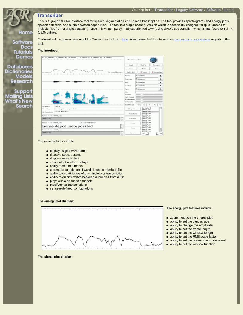
You are here: Transcriber / Legacy Software / Software / Home

Transcriber This is a graphical user interface tool for speech segmentation and speech transcription. The tool provides spectrograms and energy plots,

speech selection, and audio playback capabilities. The tool is a single channel version which is specifically designed for quick access to multiple files from a single speaker (mono). It is written partly in object-oriented C++ (using GNU's gcc compiler) which is interfaced to Tcl-Tk (v8.0) utilities.

To download the current version of the Transcriber tool click here. Also please feel free to send us comments or suggestions regarding the tool.

The interface:

The main features include

● displays signal waveforms ● displays spectrograms ● displays energy plots ● zoom in/out on the displays ● ability to set time marks ● automatic completion of words listed in a lexicon file ● ability to set attributes of each individual transcription ● ability to quickly switch between audio files from a list ● plays audio on mono channels ● modify/enter transcriptions ● set user-defined configurations

The energy plot display:

The energy plot features include

● zoom in/out on the energy plot ● ability to set the canvas size ● ability to change the amplitude ● ability to set the frame length ● ability to set the window length ● ability to set the RMS scale factor ● ability to set the preemphasis coefficient ● ability to set the window function

The signal plot display:

The signal plot features include

● zoom in/out on the signal plot ● ability to change the amplitude ● ability to change the volume ● ability to set the audio device and server

The spectrogram display:

The spectrogram features include

● zoom in/out on the spectrogram ● ability to change brightness ● ability to change the contrast ● ability to set the preemphasis coefficient ● ability to set the window function

The Transcriber tool currently supports only 16 bit single channel linear data (RAW). In order to use the Transcriber with other types of data you will need to use the NIST SPHERE tools to convert your data to RAW format.

In order to use your own data with the Transcriber you will need to set up a configuration file with parameters like the audio device, audio server, sample frequency, sample number of bytes etc. You will also need to specify the lexicon file path (lexfile) and the call file path (callfile). The lexicon file for all purposes is a user defied reference dictionary that can be viewed, searched, and modified according to one's preference. The call file contains the location of the transcription file, audio list and comment file. Each of the three previous parameters are significant in which the transcription file contains a set key value pairs that describe each entry in the file. The comment file on the other hand contains a set of bookmarks that tells you the start and stop time along with the duration of the transcription process. Finally, the audio list contains the location of all the audio data that is associated with the given transcription file.

An example directory structure of the Transcriber follows:

There are several options that are available for using the display and audio facilities. These options are accessible by clicking on the Config button on the main screen.

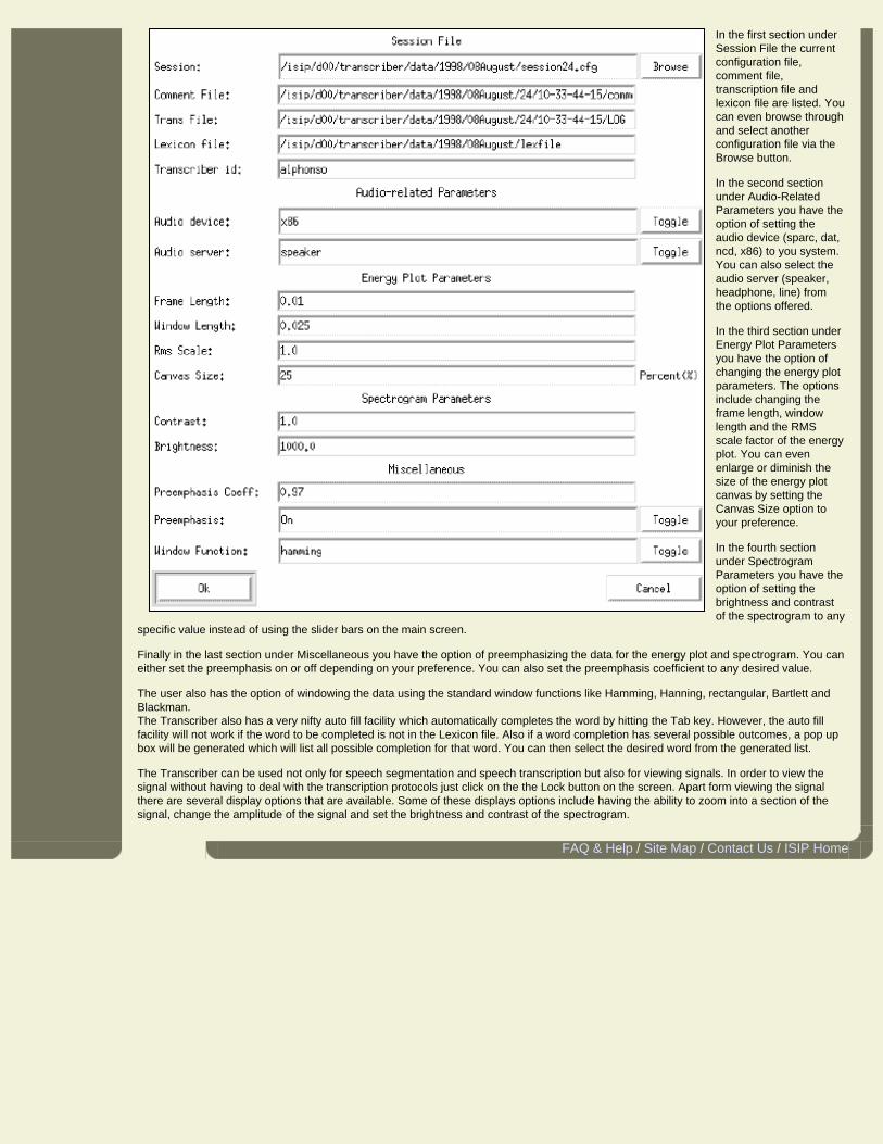
In the first section under Session File the current configuration file, comment file, transcription file and lexicon file are listed. You can even browse through and select another configuration file via the Browse button.

In the second section under Audio-Related Parameters you have the option of setting the audio device (sparc, dat, ncd, x86) to you system. You can also select the audio server (speaker, headphone, line) from the options offered.

In the third section under Energy Plot Parameters you have the option of changing the energy plot parameters. The options include changing the frame length, window length and the RMS scale factor of the energy plot. You can even enlarge or diminish the size of the energy plot canvas by setting the Canvas Size option to your preference.

In the fourth section under Spectrogram Parameters you have the option of setting the brightness and contrast of the spectrogram to any

specific value instead of using the slider bars on the main screen.

Finally in the last section under Miscellaneous you have the option of preemphasizing the data for the energy plot and spectrogram. You can either set the preemphasis on or off depending on your preference. You can also set the preemphasis coefficient to any desired value.

The user also has the option of windowing the data using the standard window functions like Hamming, Hanning, rectangular, Bartlett and Blackman. The Transcriber also has a very nifty auto fill facility which automatically completes the word by hitting the Tab key. However, the auto fill facility will not work if the word to be completed is not in the Lexicon file. Also if a word completion has several possible outcomes, a pop up box will be generated which will list all possible completion for that word. You can then select the desired word from the generated list.

The Transcriber can be used not only for speech segmentation and speech transcription but also for viewing signals. In order to view the signal without having to deal with the transcription protocols just click on the the Lock button on the screen. Apart form viewing the signal there are several display options that are available. Some of these displays options include having the ability to zoom into a section of the signal, change the amplitude of the signal and set the brightness and contrast of the spectrogram.

FAQ & Help / Site Map / Contact Us / ISIP Home

Index of /publications/courses/ase_6713

Name Last modified Size Description

Parent Directory 27-Dec-2001 14:47 -

lecture_02.fm 15-May-1998 12:16 2.7M

lecture_02.pdf 15-May-1998 17:34 224k

Apache/1.3.9 Server at www.isip.msstate.edu Port 80

Page 2.1 Speech Production Modelling E.4.14 – Speech Processing

TUBE.PPT(1/5/2001) 2.1

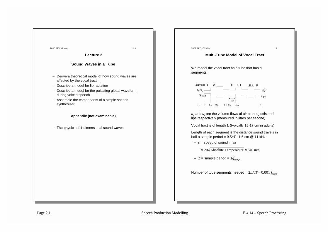
Lecture 2

Sound Waves in a Tube

– Derive a theoretical model of how sound waves are affected by the vocal tract

– Describe a model for lip radiation– Describe a model for the pulsating glottal waveform

during voiced speech– Assemble the components of a simple speech

synthesiser

Appendix (not examinable)

– The physics of 1-dimensional sound waves

TUBE.PPT(1/5/2001) 2.2

Multi-Tube Model of Vocal Tract

We model the vocal tract as a tube that has psegments:

Glottis Lips

1 2 pk k+1 p-1Segment:

u (t)lu (t)g

L/p

x = 0 L/p 2L/p (k–1 )L/p kL/p L

ug and ul are the volume flows of air at the glottis and lips respectively (measured in litres per second).

Vocal tract is of length L (typically 15-17 cm in adults)

Length of each segment is the distance sound travels in half a sample period = 0.5cT : 1.5 cm @ 11 kHz

– c = speed of sound in air

– T = sample period = 1/fsamp

Number of tube segments needed = 2L/cT ≈ 0.001 fsamp

m/s340eTemperaturAbsolute20 ≈≈

Page 2.2 Speech Production Modelling E.4.14 – Speech Processing

TUBE.PPT(1/5/2001) 2.3

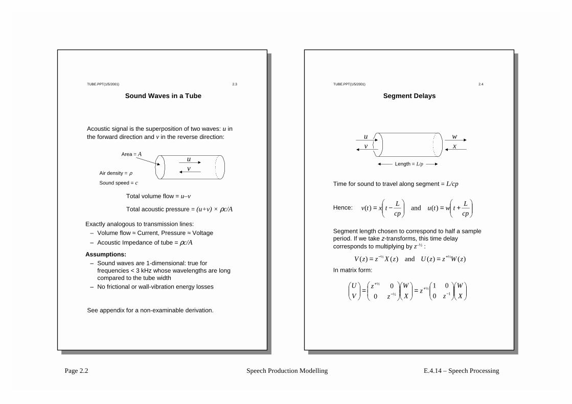
Sound Waves in a Tube

Exactly analogous to transmission lines:– Volume flow ≈ Current, Pressure ≈ Voltage– Acoustic Impedance of tube = ρc/A

Assumptions:– Sound waves are 1-dimensional: true for

frequencies < 3 kHz whose wavelengths are long compared to the tube width

– No frictional or wall-vibration energy losses

See appendix for a non-examinable derivation.

Acoustic signal is the superposition of two waves: u in the forward direction and v in the reverse direction:

Total volume flow = u–v

Total acoustic pressure = (u+v) × ρc/A

uv

Area = A

Air density = ρ

Sound speed = c

TUBE.PPT(1/5/2001) 2.4

Segment Delays

uv

wx

Length = L/p

Time for sound to travel along segment = L/cp

Hence:

Segment length chosen to correspond to half a sample period. If we take z-transforms, this time delay corresponds to multiplying by z–½ :

In matrix form:

+=

−=

cpLtwtu

cpLtxtv )(and)(

)()(and)()( ½½ zWzzUzXzzV +− ==

=

=

−

+−

+

XW

zz

XW

zz

VU

1½

½

½

001

00

Page 2.3 Speech Production Modelling E.4.14 – Speech Processing

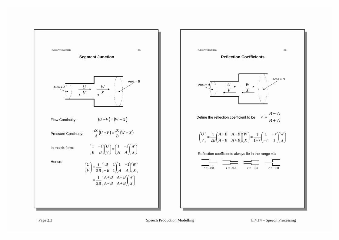
TUBE.PPT(1/5/2001) 2.5

Segment Junction

UV

WX

Area = AArea = B

Flow Continuity:

Pressure Continuity:

In matrix form:

Hence:

( ) ( )XWBcVU

Ac +=+ ρρ

( ) ( )XWVU −=−

−=

−XW

AAVU

BB1111

+−−+

=

−

−=

XW

BABABABA

B

XW

AABB

BVU

21

1111

21

TUBE.PPT(1/5/2001) 2.6

Reflection Coefficients

UV

WX

Area = AArea = B

Define the reflection coefficient to beABABr

+−=

−−

+=

+−−+

=

XW

rr

rXW

BABABABA

BVU

11

11

21

r = –0.8 r = –0.4 r = +0.4 r = +0.8

Reflection coefficients always lie in the range ±1:

Page 2.4 Speech Production Modelling E.4.14 – Speech Processing

TUBE.PPT(1/5/2001) 2.7

2-Segment Vocal Tract

Ug

Vg

Ul

Vl=0

r0r1

r2

A1 A2

×

×

−−

+=

−1

½

0

0

0 001

11

11

zz

rr

rVU

g

g

×

×

−−

+ −1½

1

1

1 001

11

11

zz

rr

r

−−

+ 011

11

2

2

2

lUr

rr

• Assume Vl = 0: no sound reflected back into mouth

• Work backwards from lips towards glottis:– Junction: use the reflection matrix– Tube segment: use the delay matrix

• A3 is large but not infinite: assumption of narrow tube breaks down at this point

• A0 is approximately zero: area of glottis opening

kk

kkk AA

AAr+−=

+

+

1

1

TUBE.PPT(1/5/2001) 2.8

Vocal Tract Transfer Function

( )( )

( ) l

kk

g

g Uzrzrrrrrzrrzrrrr

r

zVU

−+−−+++

+=

−−

−−

=

+

∏2

21

21010

220

12110

2

0

1 1

1

( )( )

( )

22

11

1

220

12110

1

220

12110

12

0

1

1

1

1

−−

−

−−

−

−−

−

=

−−=

+++=

+++

×+=

∏

zazaGz

zrrzrrrrGz

zrrzrrrr

zr

UU k

k

g

l

Ug

Vg

Ul

Vl=0

r0r1

r2

A1 A2

Multiplying out the matrices gives:

We can ignore Vg: it gets absorbed in the lungs.

The vocal tract transfer function is given by the ratio of Ul to Ug:

Page 2.5 Speech Production Modelling E.4.14 – Speech Processing

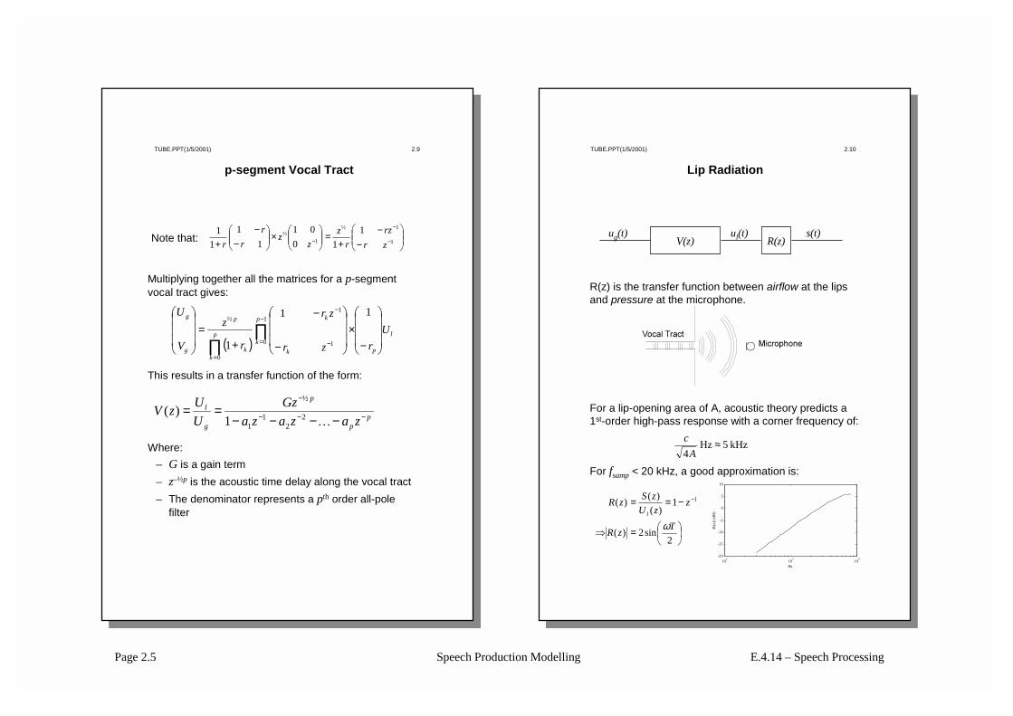
TUBE.PPT(1/5/2001) 2.9

p-segment Vocal Tract

pp

p

g

l

zazazaGz

UUzV −−−

−

−−−−==

�

22

11

½

1)(

Multiplying together all the matrices for a p-segment vocal tract gives:

( )l

p

p

kk

k

p

kk

p

g

g

Urzr

zr

r

z

V

U

−×

−

−

+=

∏∏

−

= −

−

=

11

1

1

0 1

1

0

½

−−

+=

×

−−

+ −

−

− 1

1½

1½ 1

1001

11

11

zrrz

rz

zz

rr

rNote that:

This results in a transfer function of the form:

Where:– G is a gain term– z–½p is the acoustic time delay along the vocal tract– The denominator represents a pth order all-pole

filter

TUBE.PPT(1/5/2001) 2.10

Lip Radiation

R(z) is the transfer function between airflow at the lips and pressure at the microphone.

For a lip-opening area of A, acoustic theory predicts a 1st-order high-pass response with a corner frequency of:

For fsamp < 20 kHz, a good approximation is:

V(z) R(z)ug(t) ul(t) s(t)

=⇒

−== −

2sin2)(

1)()()( 1

TzR

zzUzSzR

l

ω

102

103

104

-20

-15

-10

-5

0

5

10

Hz

|R(z

)| (d

B)

kHz5Hz4

≈A

c

Page 2.6 Speech Production Modelling E.4.14 – Speech Processing

TUBE.PPT(1/5/2001) 2.11

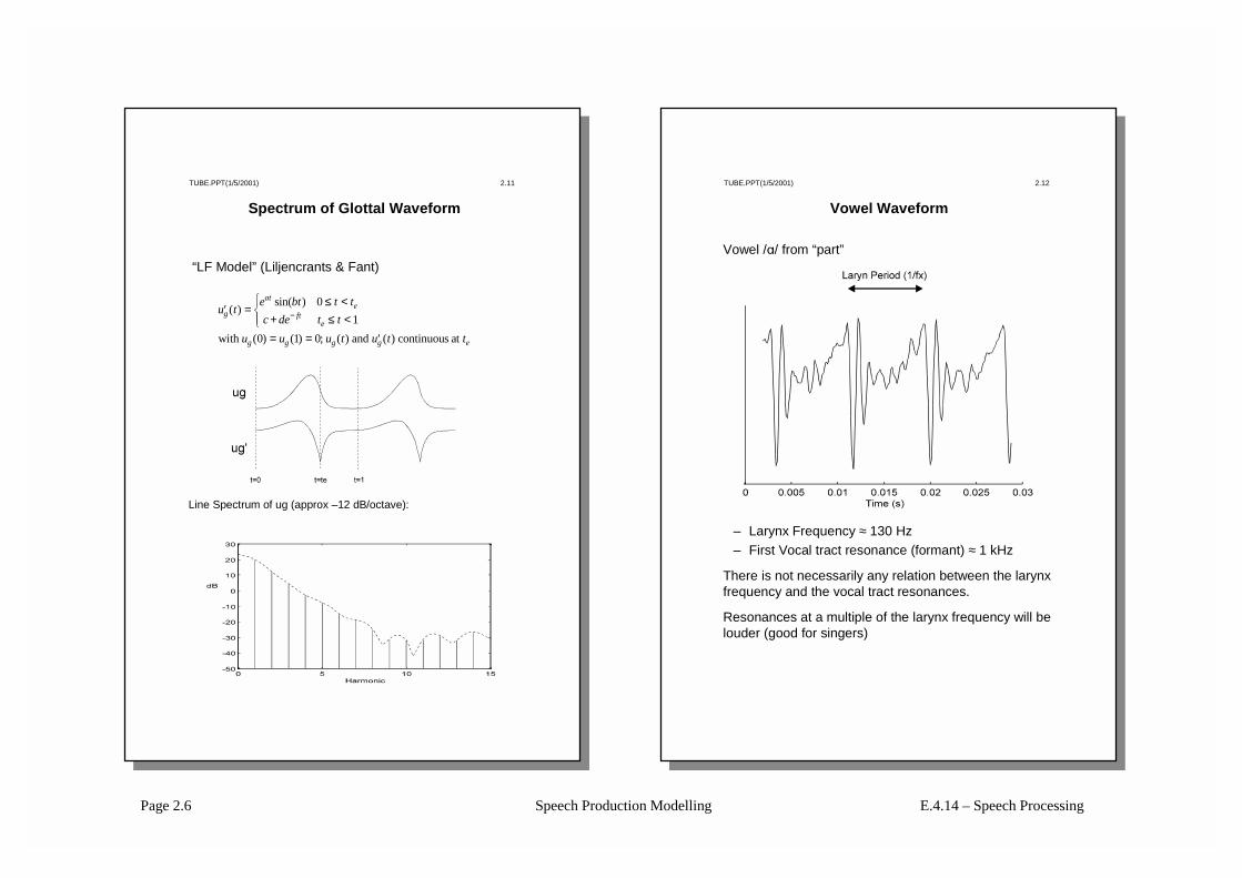
Spectrum of Glottal Waveform

“LF Model” (Liljencrants & Fant)

Line Spectrum of ug (approx –12 dB/octave):

′ =≤ <

+ ≤ <

= = ′

−u t e bt t tc de t t

u u u t u t t

g

ate

fte

g g g g e

( ) sin( )

( ) ( ) ; ( ) ( )

01

0 1 0with and continuous at

TUBE.PPT(1/5/2001) 2.12

Vowel Waveform

– Larynx Frequency ≈ 130 Hz– First Vocal tract resonance (formant) ≈ 1 kHz

There is not necessarily any relation between the larynx frequency and the vocal tract resonances.

Resonances at a multiple of the larynx frequency will be louder (good for singers)

Vowel /A/ from “part”

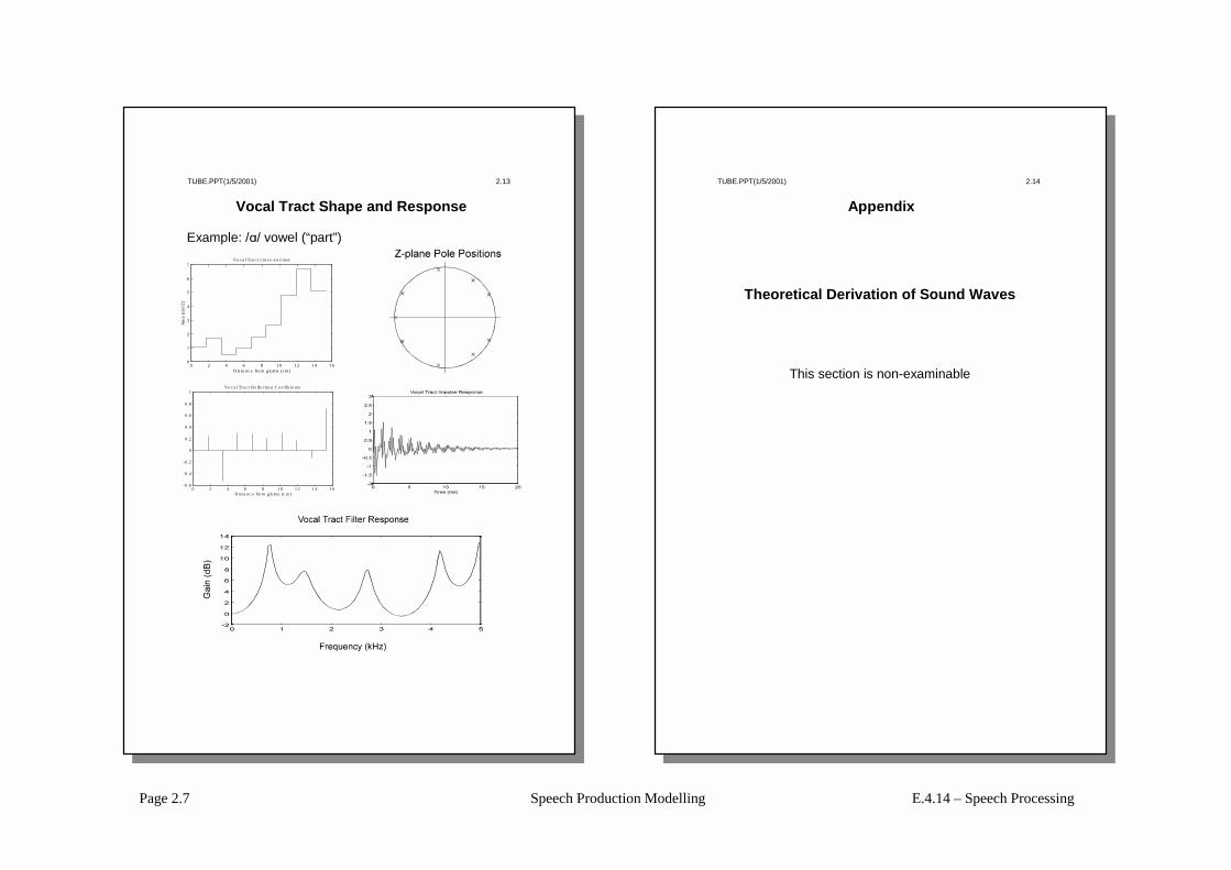
Page 2.7 Speech Production Modelling E.4.14 – Speech Processing

TUBE.PPT(1/5/2001) 2.13

Vocal Tract Shape and Response

Example: /A/ vowel (“part”)

0 2 4 6 8 1 0 1 2 1 4 1 60

1

2

3

4

5

6

7Vo c a l Tra c t cros s -s e c tio n

D is ta nc e from g lo ttis (c m )

Are

a (c

m^2

)

0 2 4 6 8 1 0 1 2 1 4 1 6-0 .6

-0 .4

-0 .2

0

0 .2

0 .4

0 .6

0 .8

1Vo c a l Tra c t R e fle c tio n C o e ffic ie nts

D is ta nc e fro m g lo ttis (c m )

TUBE.PPT(1/5/2001) 2.14

Appendix

Theoretical Derivation of Sound Waves

This section is non-examinable

Page 2.8 Speech Production Modelling E.4.14 – Speech Processing

TUBE.PPT(1/5/2001) 2.15

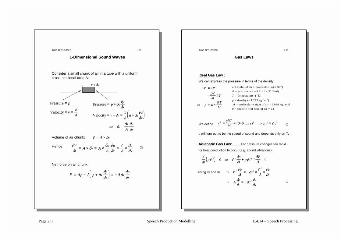
1-Dimensional Sound Waves

Consider a small chunk of air in a tube with a uniform cross-sectional area A:

Volume of air chunk:

Hence:

Net force on air chunk:

Pressure

Velocity

=

= =

p

vuA

Pressure

Velocity

= +

= + = +

⇒ =

p xpx

v vA

u xux

vxA

ux

δ∂∂

δ δ∂∂

δδ ∂

∂

1

x x x+δ

V A x= ×δ

∂∂

δδ ∂

∂∂∂

Vt

A v AxA

ux

VA

ux

= × = × = × �

F Ap A p xpx

A xpx

= − +

= −δ

∂∂ δ

∂∂

TUBE.PPT(1/5/2001) 2.16

Gas Laws

Ideal Gas Law :We can express the pressure in terms of the density:

We define

c will turn out to be the speed of sound and depends only on T.

Adiabatic Gas Law: For pressure changes too rapid

for heat conduction to occur (e.g. sound vibrations):

( )ddt

pV Vpt

p VVt

γ γ γ∂∂

γ∂∂

= ⇒ + =−0 01

cRTM

p c2 2 2340= ≈ ⇒ =γ

γ ρ( )m / s

pV nRTV

MRT

pRTM

=

=

⇒ = ×

ρ

ρ

nRT

M

= ÷ ×= = ⋅= °

= ≈= =

=

moles of air = molecules (6 10gas constant J K mol)Temperature ( K)density ( 1.225 kg / m )

molecular weight of air kg / mol= specific heat ratio of air

23

3

). / (

..

8 314

0 0291 4

ρ

γ

⇒ = − × ×

⇒ = −

Vpt

cVA

ux

Apt

cux

γγ∂

∂ρ

∂∂

∂∂

ρ∂∂

2

2

�

using � and �

�

Page 2.9 Speech Production Modelling E.4.14 – Speech Processing

TUBE.PPT(1/5/2001) 2.17

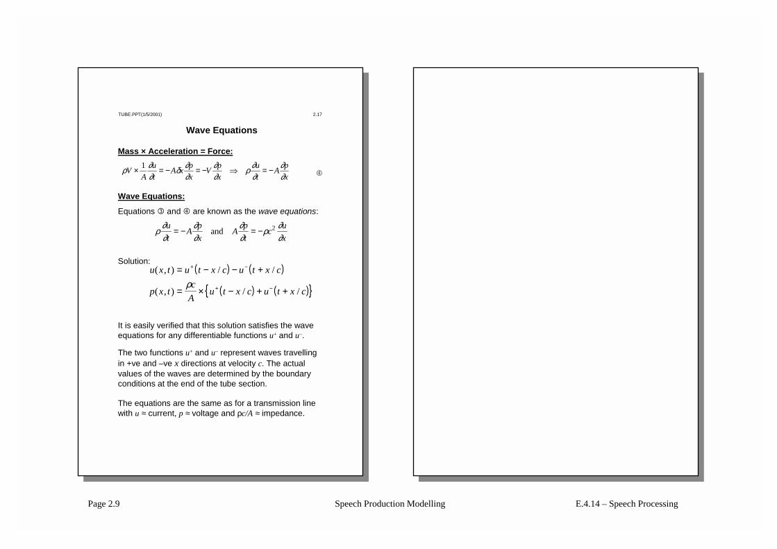
Wave Equations

Mass × Acceleration = Force:

Wave Equations:

Equations � and � are known as the wave equations:

Solution:

It is easily verified that this solution satisfies the wave equations for any differentiable functions u+ and u–.

The two functions u+ and u– represent waves travelling in +ve and –ve x directions at velocity c. The actual values of the waves are determined by the boundary conditions at the end of the tube section.

The equations are the same as for a transmission line with u ≈ current, p ≈ voltage and ρc/A ≈ impedance.

ρ ∂∂

∂∂

∂∂

ρ ∂∂

ut

Apx

Apt

cux

= − = −and 2

( ) ( )

( ) ( ){ }u x t u t x c u t x c

p x tc

Au t x c u t x c

( , ) / /

( , ) / /

= − − +

= × − + +

+ −

+ −ρ

ρ ∂∂

δ ∂∂

∂∂

ρ ∂∂

∂∂

VA

ut

A x px

V px

ut

A px

× = − = − ⇒ = −1�

EE 225D LECTURE ON ACOUSTIC TUBE MODELS

N.MORGAN / B.GOLD LECTURE 13 13.1

University of CaliforniaBerkeley

College of EngineeringDepartment of Electrical Engineering

and Computer Sciences

Professors : N.Morgan / B.GoldEE225D Spring,1999

Acoustic Tube Models

Lecture 13

EE 225D LECTURE ON ACOUSTIC TUBE MODELS

N.MORGAN / B.GOLD LECTURE 13 13.2

Introduction :

Acoustic Tube Models of English Phonemes 2 tube model.

Assumptions :

- Plane waves

- Lossless tubes

- Rigid walls

- Friction

- Thermal effect

EE 225D LECTURE ON ACOUSTIC TUBE MODELS

N.MORGAN / B.GOLD LECTURE 13 13.3

Vocal tract area for four vowel sounds

EE 225D LECTURE ON ACOUSTIC TUBE MODELS

N.MORGAN / B.GOLD LECTURE 13 13.4

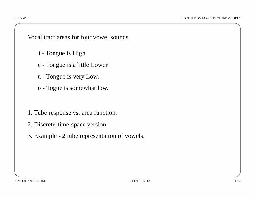
Vocal tract areas for four vowel sounds.

1. Tube response vs. area function.

2. Discrete-time-space version.

3. Example - 2 tube representation of vowels.

i - Tongue is High.

e - Tongue is a little Lower.

u - Tongue is very Low.

o - Togue is somewhat low.

EE 225D LECTURE ON ACOUSTIC TUBE MODELS

N.MORGAN / B.GOLD LECTURE 13 13.5

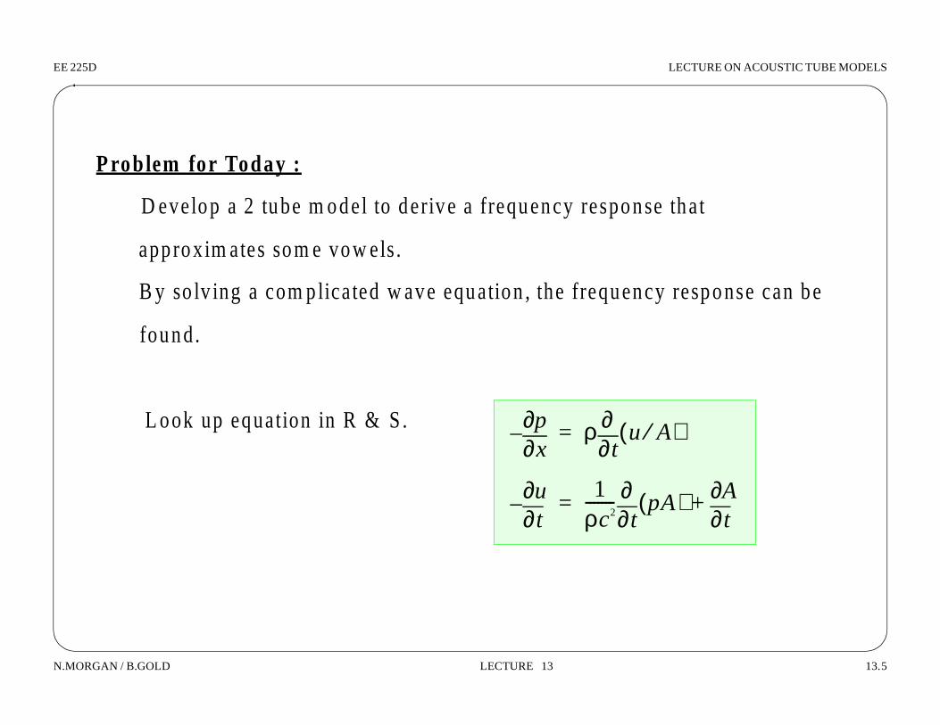
P rob lem for Today :

D evelop a 2 tube m odel to derive a frequency response that

approx im ates som e vow els.

B y so lv ing a com p licated w ave equation , the frequency response can be

L ook up equation in R & S .x∂

∂p– ρt∂

∂ u A⁄( )=

t∂∂u–

1ρc2-------

t∂∂ pA( )

t∂∂A+=

found.

EE 225D LECTURE ON ACOUSTIC TUBE MODELS

N.MORGAN / B.GOLD LECTURE 13 13.6

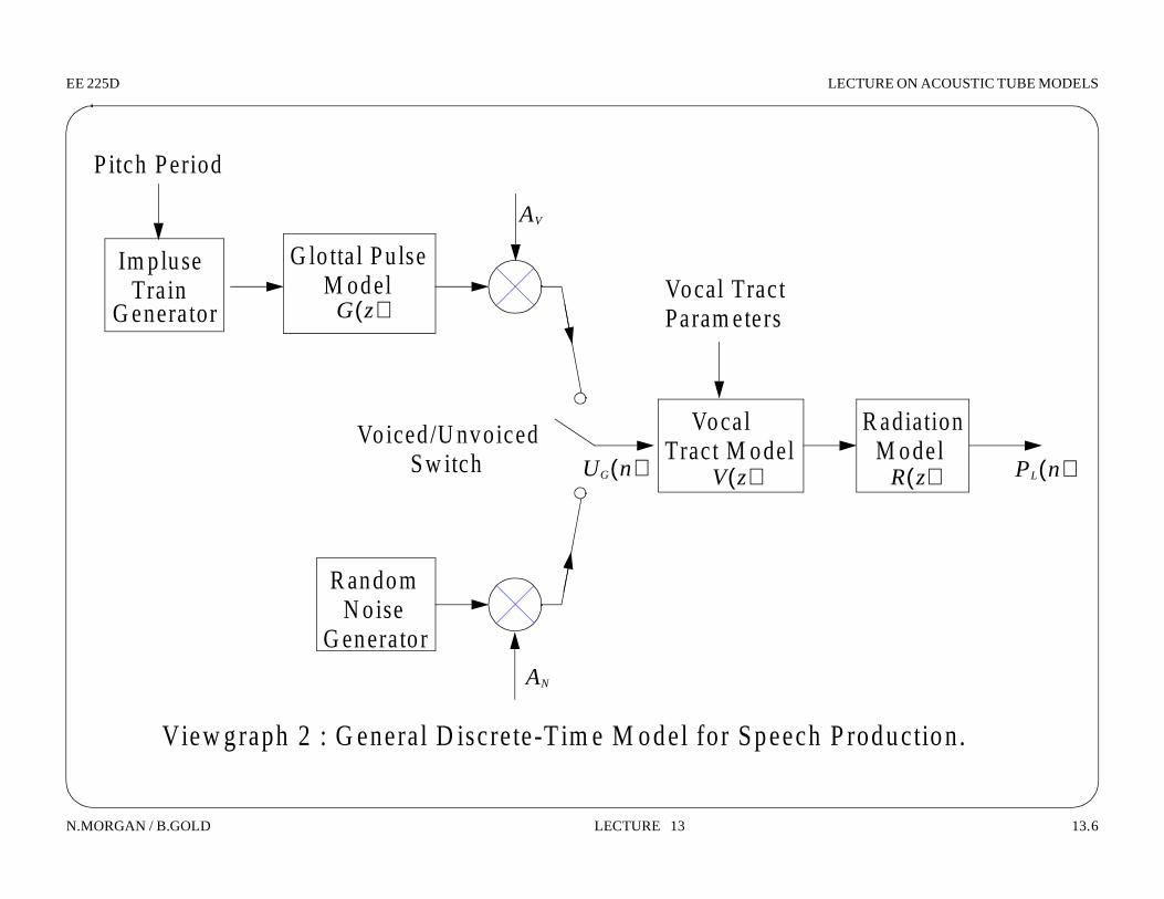
View graph 2 : G eneral D iscrete-T im e M odel for Speech P roduction.

P itch Period

Im p luse G lo tta l Pu lse

Vo iced /U nvoiced

Vocal Tract

Vocal R adiation

R andom

Tra in G enerator

M odel

Sw itch

N o ise G enerato r

Tract M odel M odel V z( ) R z( )

G z( )

UG n( )

AV

AN

PL n( )

Param eters

EE 225D LECTURE ON ACOUSTIC TUBE MODELS

N.MORGAN / B.GOLD LECTURE 13 13.7

A ssum ption in th is M odel :

Vocal Tract M odel - T im e vary ing

R ad iation M odel - M ay be tim e vary ing

G lo tta l Pu lse M odel - U sually considered independen t o f vocal tract

m odel, bu t la ter w e’ll exam ine th is w ave c losely

u x t,( ) u + t xC----–

u – t xC----+

–=

p x t,( ) Zo u + t xC----–

u – t xC----+

+=

p l t,( ) 0 : open tube=

u + t lC----–

u – t lC----+

–=

u l t,( ) 2u + t lC----–

=

EE 225D LECTURE ON ACOUSTIC TUBE MODELS

N.MORGAN / B.GOLD LECTURE 13 13.8

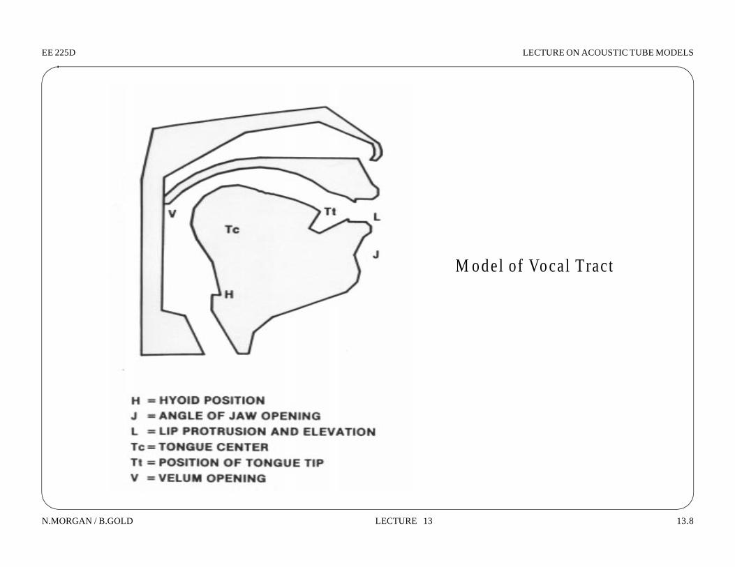
M odel of Vocal Tract

EE 225D LECTURE ON ACOUSTIC TUBE MODELS

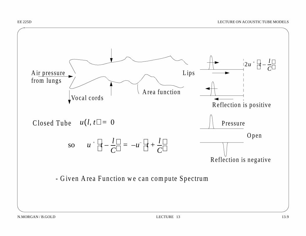
N.MORGAN / B.GOLD LECTURE 13 13.9

A ir pressure

Vocal cordsA rea function

L ips

C losed Tube

from lungs

R eflec tion is positive

Pressure

O pen

R eflection is negative

2u + t lC----–

u l t,( ) 0=

so u + t lC----–

u – t lC----+

–=

- G iven A rea F unction w e can com pute Spectrum

EE 225D LECTURE ON ACOUSTIC TUBE MODELS

N.MORGAN / B.GOLD LECTURE 13 13.10

F igure 11 .1: X -ray tracing and area function fo r phonem e /i/

EE 225D LECTURE ON ACOUSTIC TUBE MODELS

N.MORGAN / B.GOLD LECTURE 13 13.11

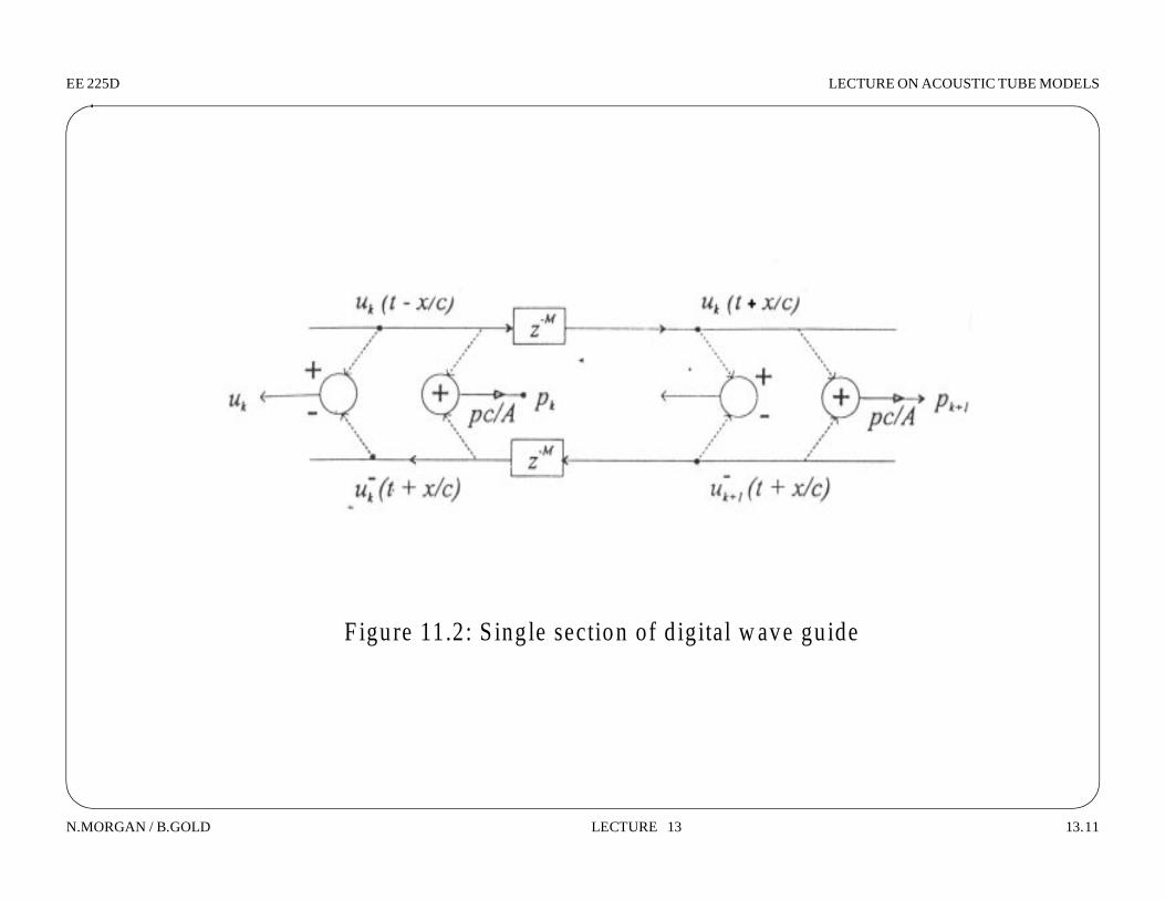
F igure 11.2: S ing le section of d ig ital w ave gu ide

EE 225D LECTURE ON ACOUSTIC TUBE MODELS

N.MORGAN / B.GOLD LECTURE 13 13.12

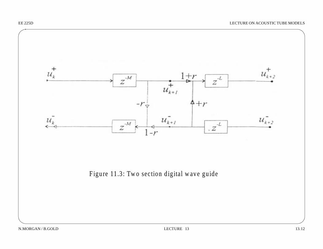
F igure 11.3: Tw o section d ig ital w ave gu ide

EE 225D LECTURE ON ACOUSTIC TUBE MODELS

N.MORGAN / B.GOLD LECTURE 13 13.13

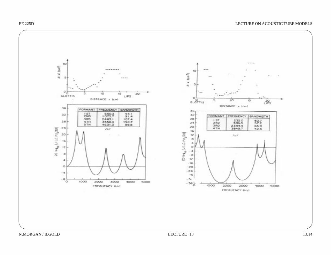
F igure 3.24 A rea function and frequency response for the R ussian vow el /e/

F igure 3.25 A rea function and frequency response for the R ussian vow el /i /

EE 225D LECTURE ON ACOUSTIC TUBE MODELS

N.MORGAN / B.GOLD LECTURE 13 13.14

EE 225D LECTURE ON ACOUSTIC TUBE MODELS

N.MORGAN / B.GOLD LECTURE 13 13.15

a)

A1 A2 A3 A4 A5

x∆x∆

x∆ ∞x∆

b)1 r 1+( ) 1 r 2+( ) 1 r 3+( ) 1 r 4+( )z 2–

1 r 3–( )1 r 2–( )1 r 1–( )

uG n( ) uL n( )

r 1– r 1r 2– r 3– r 4– r L–=r 2 r 3

M ore C om plex Tube S tructure

EE 225D LECTURE ON ACOUSTIC TUBE MODELS

N.MORGAN / B.GOLD LECTURE 13 13.16

F igu re 11 .4 F orm ants 1 and 2 ob ta ined from tw o tube m odel

Physics!

Physics in Speech

An introduction to some of the physics in speech(including some notes about helium speech)

Content : Joe Wolfe

This short document describes a simple model of the vocal tract and the production of voiced speech used in the production of some sustained phonemes - especially the vowels. It also includes some brief notes about helium speech.

The source-filter model of the vocal tract

The vibration of the vocal folds produces a varying air flow which may be treated as a periodic source (A). (A periodic signal is cyclic: its motion is reproduced after a time interval called its period. A consequence is that its spectrum is made up of harmonics. Go to 'What is a sound spectrum?' for an introduction.) This source signal is input to the vocal tract. The tract behaves like a variable filter (B) in that its response is different for different frequencies. It is variable because, by changing the position of your tongue, jaw etc you can change that frequency response. The input signal and the vocal tract, together with the radiation properties of the mouth, face and external field, produce a sound output (C). Because the source is harmonic, we can say that the gain of the tract (B) is sampled at multiples of the pitch frequency F0. In the case at left, the resonances R1 and R2 can be determined approximately from the peaks in the envelope of the sound spectrum. These peaks are called the formants (F1 and F2).

Note that the detail in the spectrum is easier to see if F0 is low, e.g. for a low pitched man's voice (diagram at left), than it is for a child's or woman's voice - shown at right.

The lowest resonance is determined to a considerable extent by the end effect of your mouth: if you lower your jaw, R1 rises. R2 is affected by the jaw position too, but it is primarily affected by the position of the constriction inside your mouth. Moving your tongue forwards and backwards changes R2 (and also R1, but to a lesser extent). A map of (R1,R2) for Australian English is given on our speech research page.

Nearly all information in speech is in the range 200 Hz-8 kHz. (The telephone carries only 300 Hz - 3 kHz but speech is reasonably intelligible and the telephone company's hold music still sounds okay.) The pitch is determined by the spacing of harmonics as much as or more than by the fundamental. Thus you can tell the pitch of a man's voice on the phone even though the fundamental of that signal is not present. Note the size of the vocal tract (~170 mm long) gives resonances > ~ 500 Hz. In fact a closed tube of this length is a functional approximation of the tract for the vowel "er" as in "herd". For this 'neutral' vowel, the first five resonances of the author's vocal tract are indeed at values of about 500, 1500, 2500, 3500 and 4500 Hz.

You can investigate this model by changing the speed of sound. Inhaling helium changes the frequencies of the resonances. As you would expect, it does not change the pitch, which is determined by the tension, mass and geometry of vocal folds, and some other effects. It does however change the timbre. In speech, you may have the illusion that the pitch has changed because one doesn't think much about pitch when listening to speech. To make it clear, you can sing with and without a lung full of He and listen.

Warnings:

● He is suffocating and conducts heat well. ● After one inhalation of He, breathe air normally for a few minutes. ● In a gas cylinder, He is under high pressure. ● Do not inhale directly from a gas cylinder. ● Fill a toy balloon and inhale from that.

What helium does to speech

The first diagram shows a schematic picture of the spectrum for a particular configuration of the vocal tract filled with air. The solid line is the spectral envelope; the vertical lines are the harmonics of the vibration of the vocal folds. The second diagram shows the effect of replacing air with helium, but keeping the tract configuration the same (i.e. trying to pronounce the same vowel as before, but with a throat full of helium). The speed of sound is greater, so the resonances occur at higher frequencies: the second resonance has been shifted right off scale in this diagram. The flesh in your vocal folds still vibrates at the same* frequency, so the harmonics occur at the same frequency.

What does this sound like? Well if you listen for the pitch, you will hear that it is the same note as previously (it is easier to hear the pitch if you sing rather than speak, because in speech we are much less conscious of the pitch). If you do the experiment with someone who has a bit of experience with singing, (and if s/he doesn't laugh too much on hearing helium voice) then the pitch will be the same in the two cases. The pitch is determined by the frequencies of the harmonics and these have not changed*. The speech does however sound 'like Donald Duck'. There is less power at low frequencies so the sound is thin and squeaky. This alteration to the timbre changes vowels in a spectacular way. Although we can understand whole sentences (using contextual clues) we find that individual vowels are very difficult to identify. (By the way, an articulate but otherwise standard duck would have a shorter vocal tract than ours so, even while breathing air, Donald would have resonances at rather higher frequencies than ours.)

* If you keep the muscle tensions the same, that is, the frequencies will not change much. There could be a small change because the less dense He loads the vocal folds a bit less than the air, but this effect is slight. The effect on the resonances is large, however. Its size depends on how pure the He in your vocal tract is.)

Audio File File Format

Ordinary Speech

Helium Speech

Pitch in Air

Pitch in Helium

Some other phoneme classes (very briefly)

Fricatives (f, sh, ss etc) are produced by turbulence at a small constriction. This produces broad band sound with characteristic frequencies. Initial plosives (b, d, k etc) have a short burst of broad band sound then a characteristic transient (as the constriction opens) in the following vowel. Final plosives have a transient (as the constriction shuts) followed by short silence and then the broad band sound. The relative timing of voicing (vocal fold vibration) is important. The presence of voicing distinguishes v from f, zz from ss, b from p etc.

Gear for further investigations:A microphone and oscilloscope with a sensitive input range (~ mV) or else a pre- amplifier. Appropriate connectors. To start, try 100 ms/div on the time base, then look more closely. If the CRO is digital (or a virtual one running on your PC), the storage mode is very useful.A PC with a sound card and analysis/edit software is useful. The sampling feature is effectively a storage CRO, and the analysis feature is effectively a spectrum analyser.You can put your fingers on your throat to determine whether vocal fold vibrate or not ('voiced' or not).

Some explanatory notes

● What is a decibel? ● What is a sound spectrum? ● What is acoustic impedance and why is it important?

Related pages

● "Vocal tract acoustics" (A web resource about our work in this area) ● "Musical acoustics" (A web resource with both introductory and

research material)

● "French vowels"

Further Information

Email

● Joe Wolfe : J.Wolfe@unsw.edu.au● Musical Acoustics Group

Phone Number

● 61 2 9385 4954 (UT +10, +11 Oct-Mar)

Facsimile Number

● 61 2 9385 6060

Copyright 1999 (including images) Joe Wolfe and John Smith, UNSW. Please seek permission before reproducing this material.

[ Search | School Information | Physics Courses | Research | Graduate ][ Resources | Physics ! | Physics Main Page | UNSW Main Page |Faculty of Science ]

School of Physics - The University of New South Wales - Sydney Australia 2052Site comments physicsweb@phys.unsw.edu.au © School of Physics UNSW 2001