1

Integral Analysis for Control Volumes-I

• Governing Equations in mechanics, thermodynamics, etc., are derived for constant mass systems

• In fluid mechanics, often, the interest is not of the moving fluid but its action on the structures through which it passes

• Pressure drop in a pipe

• Forces on pipe bends

• Temperature of fuel elements in a reactor

Integral Analysis for Control Volumes-II

• There is a need to convert the laws for a fixed mass to laws for a fixed or moving (having relative velocity with the fluid) volume.

• This is accomplished by the Reynolds transport theorem

• Before we derive it let us have a quick look at laws for the fixed mass

Governing Equations for Fixed Mass-I

��∀

∀ρ===syssys

ddmMwhere;0dt

dM

Msys

sys

Conservation of Mass

Newton’s Second Law

��∀

∀ρ===syssys

dVdmVPwhere;Fdt

Pd

Msys

sys����

�

Governing Equations for Fixed Mass-II

Conservation of Angular Momentum

��∀

∀ρ×=×==syssys

dVrdmVrHwhere;Tdt

Hd

Msys

sys�����

�

Torque for the system can have three components

externalM

s TdmgrFrTsys

������+×+×= �

Due to surface forces

Due to body forces

Shaft Torque

Governing Equations for Fixed Mass-III

First law of thermodynamics

��∀

∀ρ==−=syssys

dedmeEwhere;WQdt

dE

Msys

sys ��

gz2

Vue

2

++=

Specific energy for the system can have three components

Internal kinetic potential

Second law of thermodynamics

Governing Equations for Fixed Mass-IV

��∀

∀ρ==+=syssys

dsdmsSwhereSTQ

dt

dS

Msysp

sys ��

In general, for a System, we can write

��∀

∀ρη=η=syssys

ddmNM

sys

sSII-law-Thermo

eEI-law-Thermo

Ang. Mom

Lin. Mom

1MMass

�NConservation

P�

V�

H�

Vr��×

2

Reynolds Transport Theorem-I

• This theorem converts conservation laws from Control Mass system to Control Volume System .

• We will derive this with mass balance first

• Then we shall generalize and apply to other conservation laws

• We shall not cover Thermodynamics laws here but will apply them

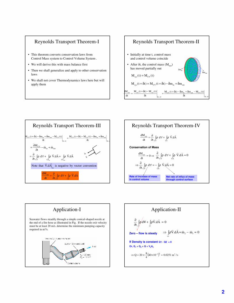
Reynolds Transport Theorem-II

• Initially at time t, control mass and control volume coincide

• After �t, the control mass (Msys) has moved partially out

)t(M)t(M CVsys =

outinCVsys mm)tt(M)tt(M δ+δ−δ+=δ+

�min�mout

0t

CVoutinCV

0t

syssyssys

t)t(Mmm)tt(M

t

)t(M)tt(M

dt

dM

→δ→δ δ−δ+δ−δ+=

δ−δ+

=

Reynolds Transport Theorem-III

0t

outinCVCV

0t

CVoutinCV

tmm)t(M)tt(M

t)t(Mmm)tt(M

→δ→δ δδ+δ−−δ+=

δ−δ+δ−δ+

outinCV mmt

M�� +−

∂∂=

��� ρ+ρ+∀ρ∂∂=

outin CSCSCV

Ad.VAd.Vdt

����

conventionvectorbynegativeisAd.VthatNotein

��

�� ρ+∀ρ∂∂=

CSCV

sys Ad.Vdtdt

dM ��

AV

Reynolds Transport Theorem-IV

�� ρ+∀ρ∂∂=

CSCV

sys Ad.Vdtdt

dM ��

Conservation of Mass

�= 0dt

dMsys 0Ad.Vdt CSCV

=ρ+∀ρ∂∂

����

0Ad.Vdt CSCV

=ρ−=∀ρ∂∂

� ����

Rate of increase of mass in control volume

Net rate of influx of mass through control surface

Application-I

Seawater flows steadily through a simple conical-shaped nozzle at the end of a fire hose as illustrated in Fig. If the nozzle exit velocity must be at least 20 m/s. determine the minimum pumping capacity required in m3/s.

0Ad.VVdt cscv

=ρ+ρ∂∂

����

Zero – flow is steady 0mmAd.V 1cs

2 =−=ρ� � ����

If Density is constant Q1 - Q2 = 0

Or, Q1 = Q2 = Q = V2A2

( ) s/m0251.010404

20Q 323 =×π×=� −

Application-II

3

Moist air (a mixture of dry air and water vapor) enters a dehumidifier at the rate of 324 kg/hr. Liquid water drains out of the dehumidifier at a rate of 7.3 kg/hr Determine the mass flow rate of the dry air and the water vapor leaving the dehumidifier. A simplified sketch of the process is provided in Fig.

hr/kg324m1 =�

hr/kg3.7m 3 =�

?m3 =�

Application-III

0Ad.VVdt cscv

=ρ+ρ∂∂

����

Zero – flow is steady

0mmmAd.V 321cs

=++−=ρ� � �����

hr/kg7.3163.7324mmm 312 =−=−=� ���

Now if we take the whole system as control volume

0mmmmm 54321 =−+−− �����

Application-IV

54 mm �� =�

Reynolds Transport Theorem-V

�� ηρ+∀ηρ∂∂=

CSCV

sys Ad.Vdtdt

dN ��

Generalization

Rate of increase of a general property in control volume

Net rate of outflux of the property through control surface

sSII-law-Thermo

eEI-law-Thermo

Ang. Mom

Lin. Mom

1MMass

�NConservation

P�

V�

H�

Vr��×

P�

V�

H�

Vr��×

Newton’s Second Law

�= ;Fdt

Pd sys�

�

Conservation of MomentumAlso called conservation of momentum

FAd.VVdVt CSCV

�����=ρ+∀ρ

∂∂

��

Let us apply it and learn the intricacies

Determine the anchoring force required to hold in place a conical nozzle attached to the end of a laboratory sink faucet shown in Fig. when the water flowrate is 0.6 liters. The nozzle mass is 0.1 kg. The nozzle inlet and exit diameters are 16 mm and 5 mm, respectively.

The nozzle axis is vertical and the axial distance between sections (1) and (2) is 30 mm. The pressure at section (1) is 464 kPa.

The anchoring force sought is the reaction force between the faucet and nozzle threads. To evaluate this force, control volume selected includes the nozzle and the water contained in the nozzle

Application-V

Wn

FA

p1A1

w1

p2A2

w2

z

FA – anchoring force that holds the nozzle in place

Wn – weight of the nozzle

Ww – weight of the water in the nozzle

P1 – gage pressure at section (1)

A1 – cross section area at section (1)

P2 – gage pressure at section (2)

A2 – cross section area at section (2)

w1 – z direction velocity at the control volume entrance (assumed uniform)

w2 – z direction velocity at the control volume exit (assumed uniform)

The action of atmospheric pressure cancels out in every direction and is not shown

Ww

Application-VI

4

wn2211A2211 WWApApFwmwm −−+−=−� ��

FAd.VVdVt CSCV

�����=ρ+∀ρ

∂∂

��

Zero – flow is steady

2211CS

m)w()m)(w(Ad.VV �����

−+−−=ρ� �

=F�

2211A ApApF +−=SF�

BF�

+ wn WW −−

Conservation of mass

mmmor0mm 2121 ����� ===−�

0Ad.VVdt cscv

=ρ+ρ∂∂

� ����

0

Application-VII

s/kg6.0106.01000QwAm 311 =××=ρ=ρ= −

�

( ) ( ) 2423211 m10011.21016

4D

4A −− ×=×π=π=

( ) ( ) 2523222 m10964.1105

4D

4A −− ×=×π=π=

s/m98.210011.2

106.0AQ

W 4

3

11 =

××== −

−

s/m6.3010964.1

106.0AQ

W 5

3

22 =

××== −

−

Application-VIII

N981.081.91.0gmW nn =×==

( )gDDDD12

hgVW 21

22

21ww ++π×ρ=ρ=

( ) ( ) ( ) ( )( )( ) N0278.081.9004.0016.0004.0016.012

03.01000W 22

w =++π×=

0p2 =�Atmospheric pressure

( ) wn221121A WWApApwwmF ++−+−=∴ �

( )( ) ( )( ) 00278.010011.2464000981.06.3098.26.0F 4A −+×++−= −

00278.03104.93981.0572.16FA −+++−=

N75.77FA =

Application-IX Reynolds Transport Theorem-VI

�� ηρ+∀ηρ∂∂=

CSrel

CV

sys Ad.Vdtdt

dN ��

For Moving Control Volumes (with constant velocity)

0Ad.Vdt CS

relCV

=ρ+∀ρ∂∂

����

Mass Balance

Momentum Balance FAd.VVdVt CS

relrelCV

rel

�����=ρ+∀ρ

∂∂

��

An airplane moves forward at a speed of 971 kmph as shown in Fig. The frontal intake area of the jet engine is 0.8m2 and the entering air density is 0.736 kg/m3. A stationary observer determines that relative to the earth, the jet engine exhaust gases move away from the engine with a speed of 1050 kmph. The engine exhaust area is 0.558 m2 and the exhaust gas density is 0.515kg/m3. Estimate the mass flow rate of fuel into the engine.

Application-X

111222infuel WAWAm ρ−ρ=�

)s/m3600/10002021)(m558.0)(m/kg515.0(m 33infuel ×=�

)s/m3600/1000971)(m8.0)(m/kg736.0( 33 ×−

s/kg5278.2=

0Ad.Vdt CS

relCV

=ρ+∀ρ∂∂

����

0

infuelinairoutairCS

rel mmmAd.V −−− −−=ρ� � ����� All relative to moving

control Volume

Application-XI

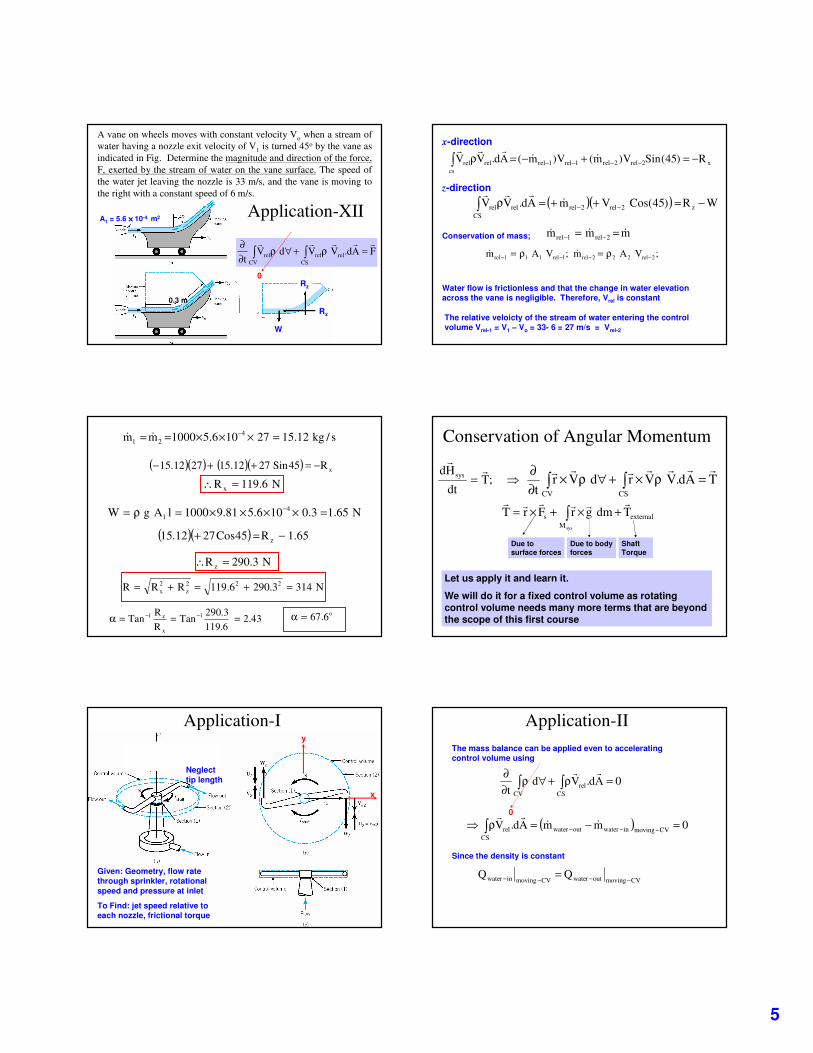
5

A vane on wheels moves with constant velocity Vo when a stream of water having a nozzle exit velocity of V1 is turned 45o by the vane as indicated in Fig. Determine the magnitude and direction of the force, F, exerted by the stream of water on the vane surface. The speed of the water jet leaving the nozzle is 33 m/s, and the vane is moving to the right with a constant speed of 6 m/s.

A1 = 5.6 ×××× 10-4 m2

W

Application-XII

0.3 m

FAd.VVdVt CS

relrelCV

rel

�����=ρ+∀ρ

∂∂

��

0Rz

Rx

x2rel2rel1rel1relcs

relrel R)45(SinV)m(V)m(Ad.VV −=+−=ρ −−−−� �����

Conservation of mass; mmm 2rel1rel ��� == −−

;VAm;VAm 2rel222rel1rel111rel −−−− ρ=ρ= ��

x-direction

z-direction

( )( ) WR)45(CosVmAd.VV z2rel2relCS

relrel −=++=ρ −−� ����

Water flow is frictionless and that the change in water elevation across the vane is negligible. Therefore, Vrel is constant

The relative veloicty of the stream of water entering the control volume Vrel-1 = V1 – Vo = 33- 6 = 27 m/s = Vrel-2

s/kg12.1527106.51000mm 421 =×××== −

��

( )( ) ( )( ) xR45Sin2712.152712.15 −=++−

N6.119R x =∴

N65.13.0106.581.91000lAgW 41 =××××=ρ= −

( )( ) 65.1R45Cos2712.15 z −=+

N3.290R z =∴

N3143.2906.119RRR 222z

2x =+=+=

43.26.1193.290

TanRR

Tan 1

x

z1 ===α −− o6.67=α

�= ;Tdt

Hd sys�

�

Conservation of Angular Momentum

TAd.VVrdVrt CSCV

�������=ρ×+∀ρ×

∂∂

��

Let us apply it and learn it.

We will do it for a fixed control volume as rotating control volume needs many more terms that are beyond the scope of this first course

externalM

s TdmgrFrTsys

������+×+×= �

Due to surface forces

Due to body forces

Shaft Torque

Application-I

Given: Geometry, flow rate through sprinkler, rotational speed and pressure at inlet

To Find: jet speed relative to each nozzle, frictional torque

x

y

Neglect tip length

Application-IIThe mass balance can be applied even to accelerating control volume using

0Ad.Vdt CS

relCV

=ρ+∀ρ∂∂

����

0

( ) 0mmAd.V CVmovinginwateroutwaterCS

rel =−=ρ� −−−� ����

Since the density is constant

CVmovingoutwaterCVmovinginwater QQ−−−− =

6

Application-IIINote that at inlet, the volume flow rate for moving control volume is same as that for fixed control volume, which is known

CVstationaryinwaterCVmovingoutwaterCVmovinginwater QQQ−−−−−− ==∴

jetrel A2

QV =∴

To get the frictional torque, we need to solve the angular momentum equation

TAd.VVrdVrt CSCV

�������=ρ×+∀ρ×

∂∂

��

This is a vector equation; but we need only the Z component

Note that we refer to fixed CV

Application-IV

externalM

s TdmgrFrTsys

������+×+×= �

We know that T has three components

1. p is atmospheric everywhere except at inlet

2. At inlet the resultant passes through r = 00Fr s =×

��

0dmgrsysM

=���

The moment on one arm is balanced by the other arm

kTTTT frictionexternal

����===∴

Application-Vrω

θ

)jsinricosr(r���

θ+θ=

)jcosrisinr()jsinVicosV(V relrel

�����θω+θω−+θ+θ=j)cosrsinV(i)sinrcosV( relrel

��θω+θ+θω−θ=

+θω+θθ=×∴ k)sinrcossinrV(Vr 22rel

���

θ

kr2�

ω=

kA3R

kAdrrdVr3R

0

2

CV

����ρω=ρω=∀ρ×� ��

Computation of transient term � ∀ρ×∂∂

CV

dVrt

��

0k3

ARt

dVrt

3

CV

=���

����

� ρω∂∂=∀ρ×

∂∂

� ����

)k)(sinrcossinrV( 22rel

�−θω−θθ

Application-VI

Computation of flux term term � ρ×CS

Ad.VVr����

QAd.VA

ρ=ρ���

jcos)RV(isin)RV(V relrel

���θω−−θω−=

)jsinRicosR(r��� θ+θ=

At outlet (Velocity assumed uniform)

At inlet r = 0; hence no contribution

kR)RV( rel

�ω−−=

QkR)RV(T rel ρω−−=∴��

Even if friction is 0, maximum � = Vrel/R

RωlReV

�

θ

θ

isin)RV(jsinRj)cos)RV((icosRVr relrel

������ θω−×θ+θω−−×θ=×

r�

Accounts for both jets

i�

j�

Conservation of Momentum in Accelerating Frame-I

�= ;Fdt

Pd sys�

�

Valid only for Inertial Frame (non-accelerating)

• For problems like a rocket taking off, we need accelerating frame analysis

• For simplicity only rectilinear accelerating frames would be considered

• An example would illustrate application

Conservation of Momentum in Accelerating Frame-II

• In the discussion XYZ frame is inertial frame and PQR would be non inertial

dtVd

dt

Vd

dtVd

VVV lRePQRXYZlRePQRXYZ

������

+=�+=

dt

d)VV(d

Fdt

dVdsyssys

lRePQR

XYZ

XYZ ��∀∀

∀+ρ==

∀ρ��

�

�

Conservation of momentum

dt

dVd

dt

dVd

FF syssys

lRePQR

PQRXYZ

��∀∀

∀ρ+

∀ρ==

��

��

7

dt

dVd

dt

dVd

F syssys

PQRlRe

PQR

��∀∀

∀ρ=

∀ρ−

��

�

dt

dVd

daF sys

sys

PQR

lRePQR

��

∀

∀

∀ρ=∀ρ−

�

��

Conservation of Momentum in Accelerating Frame-III

=∀ρ− �∀sys

daF lRePQR

��

�� ρ+∀ρ∂∂

CSPQR

CVPQR Ad.VVdV

t

����

Ve

Given

Initial Mass = 400 kg

Fuel consumption rate = 5 kg/s

Exhaust Velocity = 3500 m/s

Find

Initial acceleration

Application

Atmospheric pressure all around and air resistance neglected

y

�∀

−− ∀ρ−+sys

daFF lRePQRBPQRS

���

�� ρ+∀ρ∂∂=

CSPQR

CVPQR Ad.VVdV

t

����

0 -400 X 9.81 400 X ay 0 -3500 X 5

VPQR= const, M ~ Const.