Embed Size (px)
Citation preview
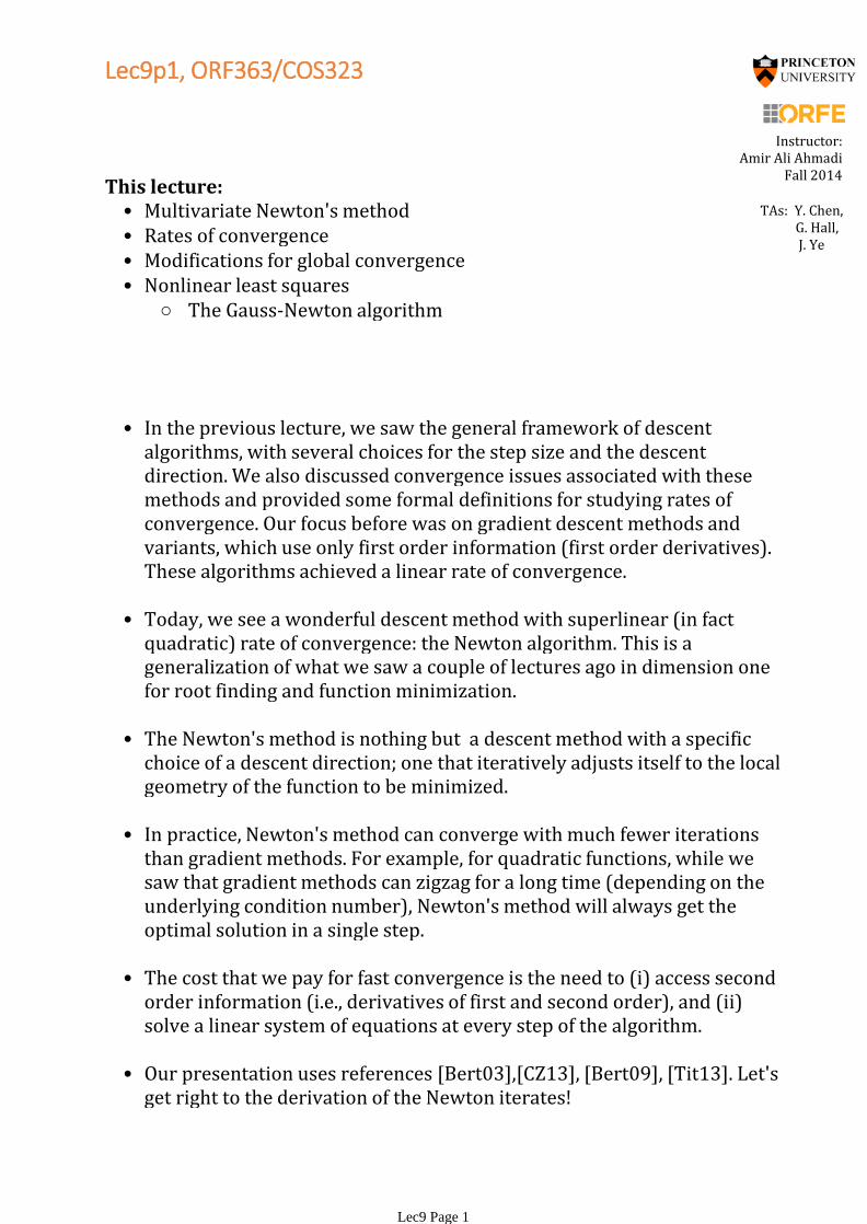
Multivariate Newton's method •• Rates of convergence
Modifications for global convergence•
○ The Gauss-Newton algorithmNonlinear least squares•
This lecture:
Instructor: Amir Ali Ahmadi
Fall 2014
In the previous lecture, we saw the general framework of descent algorithms, with several choices for the step size and the descent direction. We also discussed convergence issues associated with these methods and provided some formal definitions for studying rates of convergence. Our focus before was on gradient descent methods and variants, which use only first order information (first order derivatives). These algorithms achieved a linear rate of convergence.
•
Today, we see a wonderful descent method with superlinear (in fact quadratic) rate of convergence: the Newton algorithm. This is a generalization of what we saw a couple of lectures ago in dimension one for root finding and function minimization.
•
The Newton's method is nothing but a descent method with a specific choice of a descent direction; one that iteratively adjusts itself to the local geometry of the function to be minimized.
•
In practice, Newton's method can converge with much fewer iterations than gradient methods. For example, for quadratic functions, while we saw that gradient methods can zigzag for a long time (depending on the underlying condition number), Newton's method will always get the optimal solution in a single step.
•
The cost that we pay for fast convergence is the need to (i) access second order information (i.e., derivatives of first and second order), and (ii) solve a linear system of equations at every step of the algorithm.
•
Our presentation uses references [Bert03],[CZ13], [Bert09], [Tit13]. Let's get right to the derivation of the Newton iterates!
•
TAs: Y. Chen, G. Hall, J. Ye
Lec9p1, ORF363/COS323
Lec9 Page 1
Newton(1642-1727)
Raphson(1648-1715?)
Could not find his picture
Apparently, Raphson published his discovery of the "Newton's method" 50 years prior to Newton [Bert09]. That's what happens when people can't Google!
index of time (iteration number)
: Current point
Next point
: Direction to move along at iteration
Step size at iteration
Recall the general form of our descent methods:•
where
Let us have for now. So we take full steps at each iteration. (This is sometimes called the pureNewton method.)
•
Newton's method is simply the following choice for the descent direction:
•
Recall our notation and respectively denote the gradient and the Hessian at
○
Iteration only well-defined when the Hessian at is invertible.
○
One motivation: minimizing a quadratic approximation of the function sequentially.
•
Around the current iterate let's Taylor expand our function to second order and minimize the resulting quadratic function.
○
Where does this come from?
Lec9p2, ORF363/COS323
Lec9 Page 2
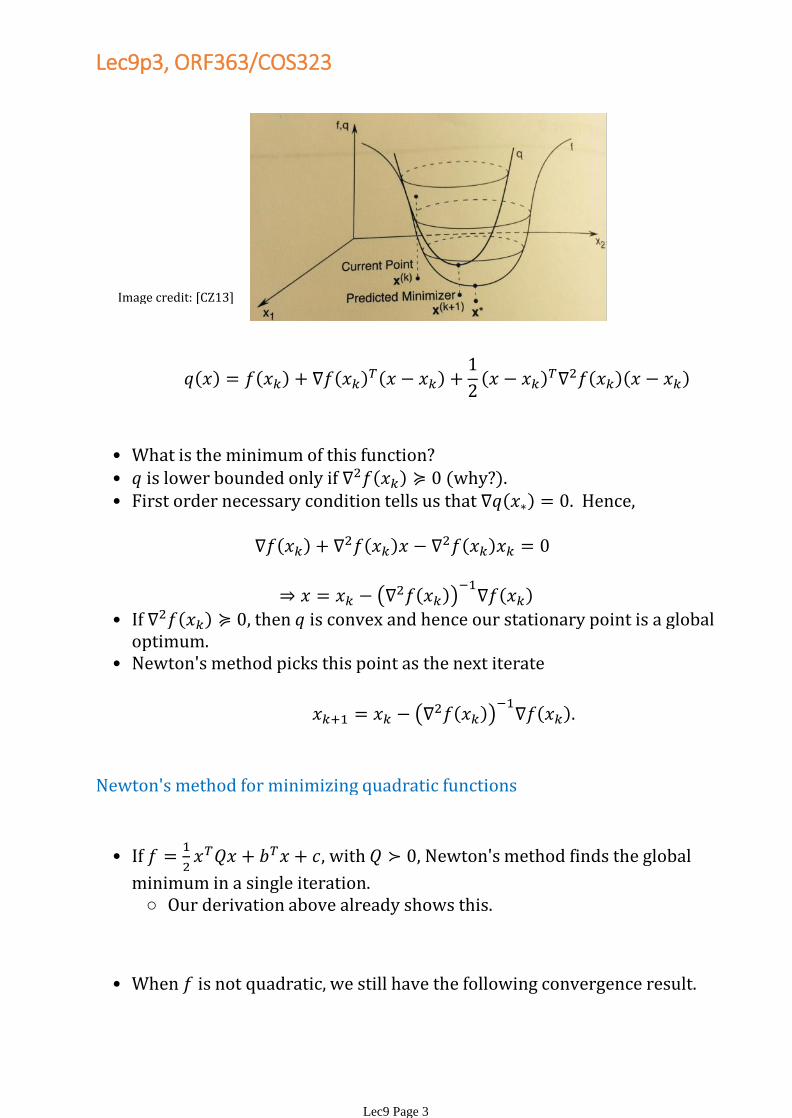
Image credit: [CZ13]
What is the minimum of this function?• is lower bounded only if (why?).•First order necessary condition tells us that Hence,•
If then is convex and hence our stationary point is a global optimum.
•
Newton's method picks this point as the next iterate•
Newton's method for minimizing quadratic functions
Our derivation above already shows this.○
If
with Newton's method finds the global
minimum in a single iteration.
•
When is not quadratic, we still have the following convergence result.•
Lec9p3, ORF363/COS323
Lec9 Page 3
Theorem. Suppose (i.e., three times continuously differentiable) and is such that and is invertible. Then, there exists such that itearations of Newton's method starting from any point are well-defined and converge to Moreover, the convergence rate is quadratic.
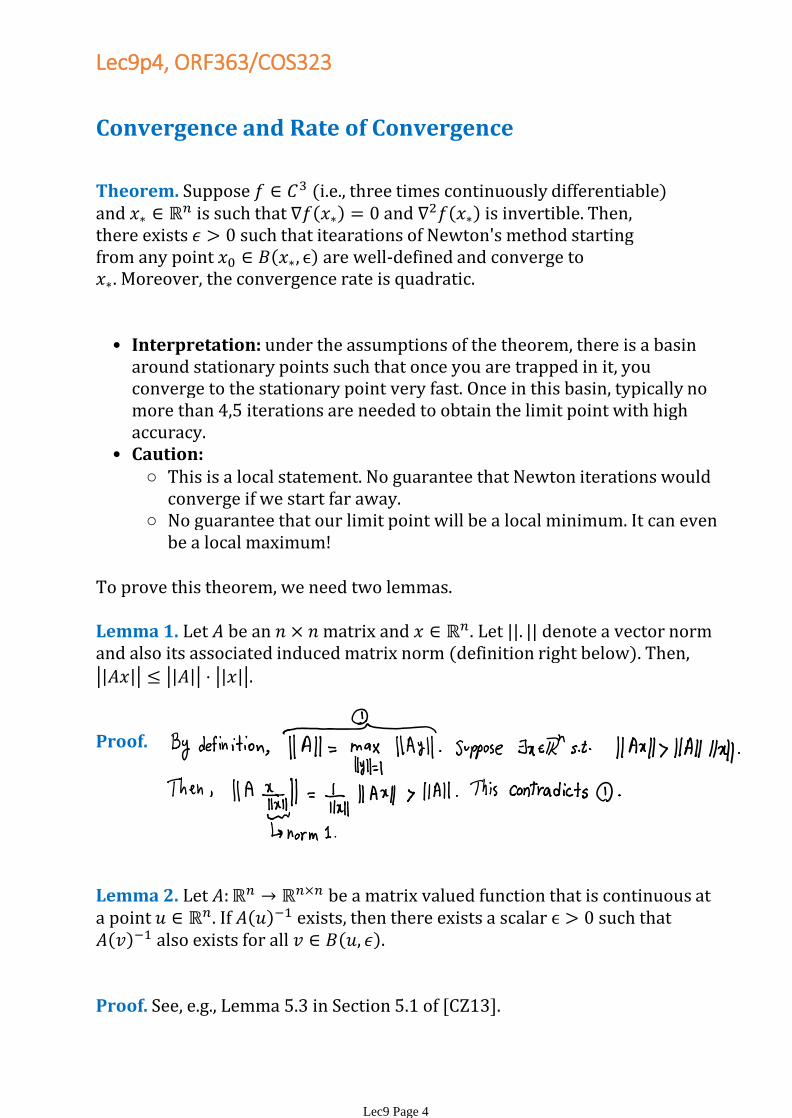
Lemma 1. Let be an matrix and Let denote a vector norm and also its associated induced matrix norm (definition right below). Then,
Interpretation: under the assumptions of the theorem, there is a basin around stationary points such that once you are trapped in it, you converge to the stationary point very fast. Once in this basin, typically no more than 4,5 iterations are needed to obtain the limit point with high accuracy.
•
This is a local statement. No guarantee that Newton iterations would converge if we start far away.
○
No guarantee that our limit point will be a local minimum. It can even be a local maximum!
○
Caution:•
To prove this theorem, we need two lemmas.
Lemma 2. Let be a matrix valued function that is continuous at a point If exists, then there exists a scalar such that also exists for all
Proof. See, e.g., Lemma 5.3 in Section 5.1 of [CZ13].
Proof.
Convergence and Rate of Convergence
Lec9p4, ORF363/COS323
Lec9 Page 4
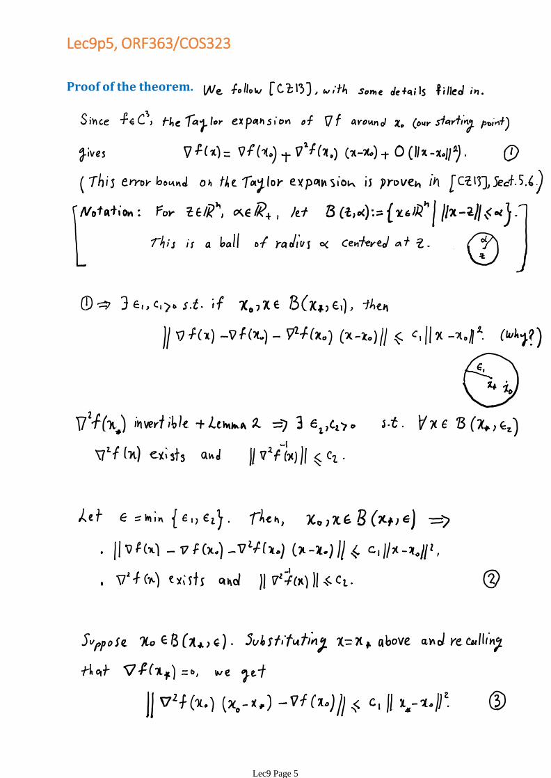
Proof of the theorem.
Lec9p5, ORF363/COS323
Lec9 Page 5
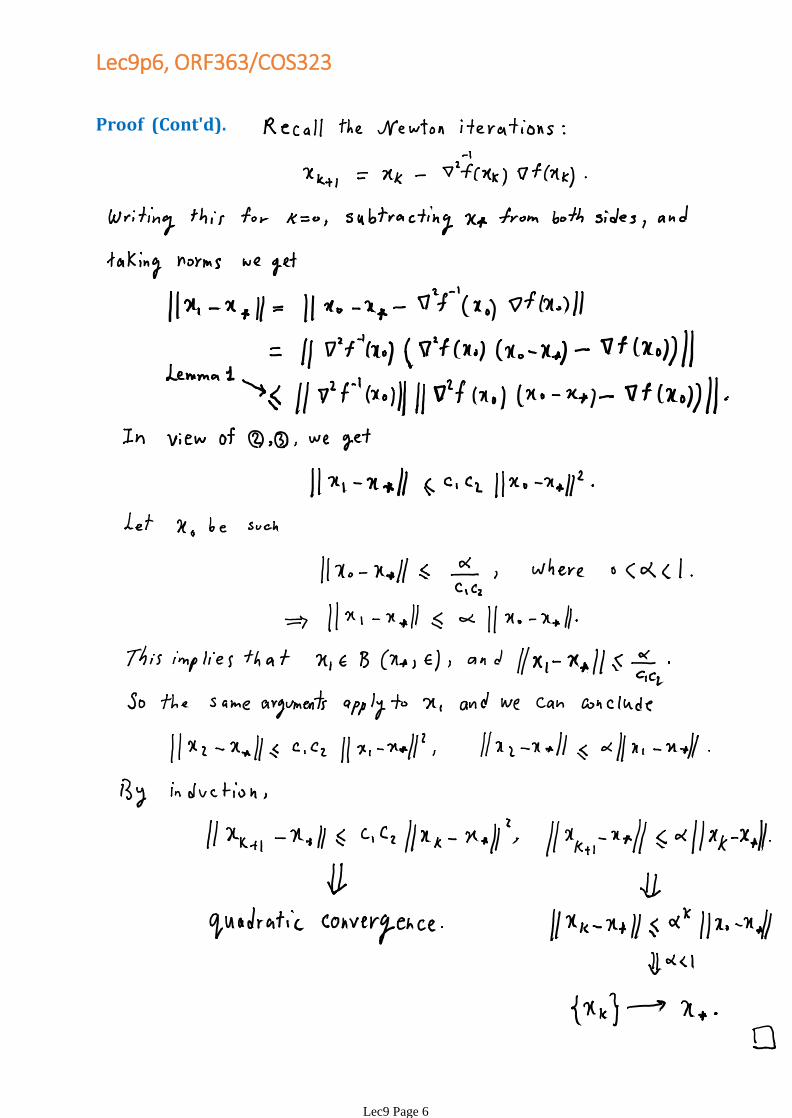
Proof (Cont'd).
Lec9p6, ORF363/COS323
Lec9 Page 6
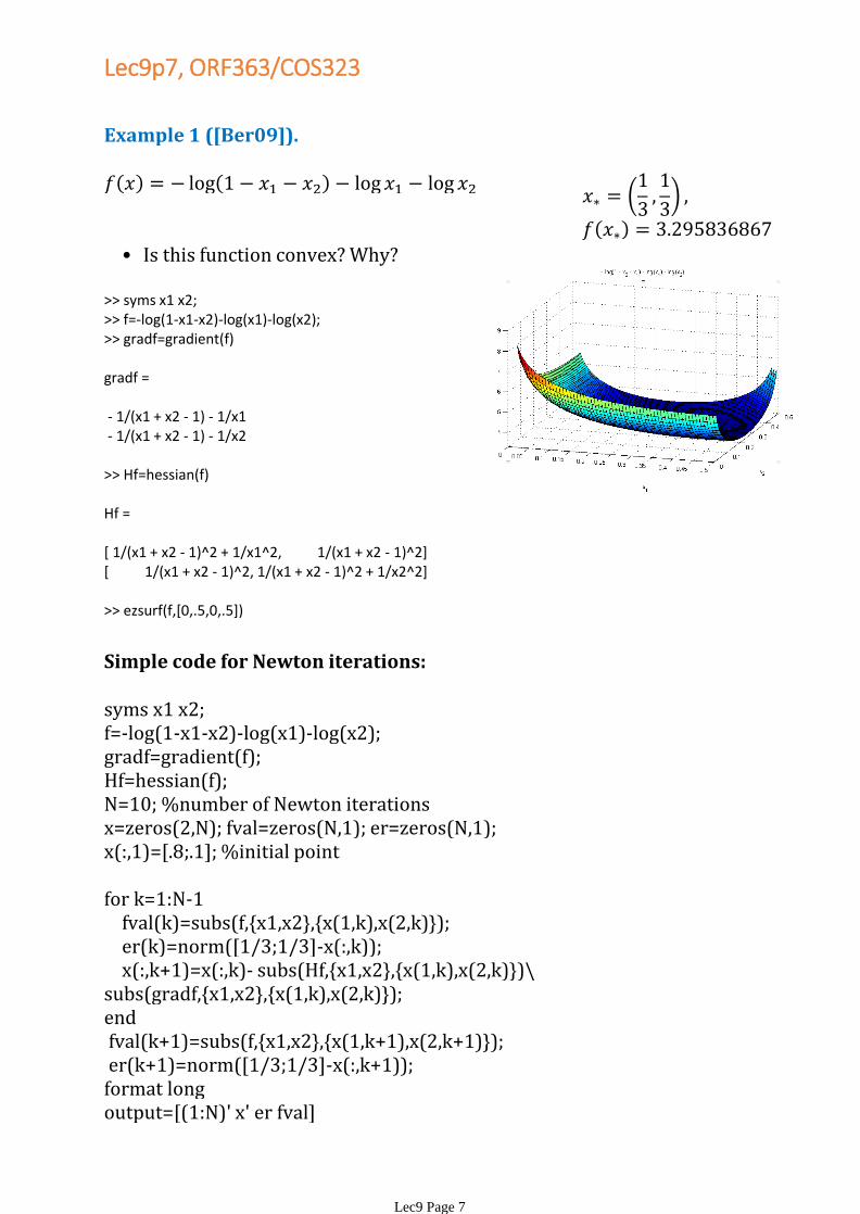
>> syms x1 x2;>> f=-log(1-x1-x2)-log(x1)-log(x2);>> gradf=gradient(f)
gradf =
- 1/(x1 + x2 - 1) - 1/x1- 1/(x1 + x2 - 1) - 1/x2
>> Hf=hessian(f)
Hf =
[ 1/(x1 + x2 - 1)^2 + 1/x1^2, 1/(x1 + x2 - 1)^2][ 1/(x1 + x2 - 1)^2, 1/(x1 + x2 - 1)^2 + 1/x2^2]
>> ezsurf(f,[0,.5,0,.5])
Example 1 ([Ber09]).
Is this function convex? Why?•
syms x1 x2;f=-log(1-x1-x2)-log(x1)-log(x2);gradf=gradient(f);Hf=hessian(f);N=10; %number of Newton iterationsx=zeros(2,N); fval=zeros(N,1); er=zeros(N,1); x(:,1)=[.8;.1]; %initial point
for k=1:N-1 fval(k)=subs(f,{x1,x2},{x(1,k),x(2,k)}); er(k)=norm([1/3;1/3]-x(:,k)); x(:,k+1)=x(:,k)- subs(Hf,{x1,x2},{x(1,k),x(2,k)})\subs(gradf,{x1,x2},{x(1,k),x(2,k)}); endfval(k+1)=subs(f,{x1,x2},{x(1,k+1),x(2,k+1)});er(k+1)=norm([1/3;1/3]-x(:,k+1));
format longoutput=[(1:N)' x' er fval]
Simple code for Newton iterations:
Lec9p7, ORF363/COS323
Lec9 Page 7
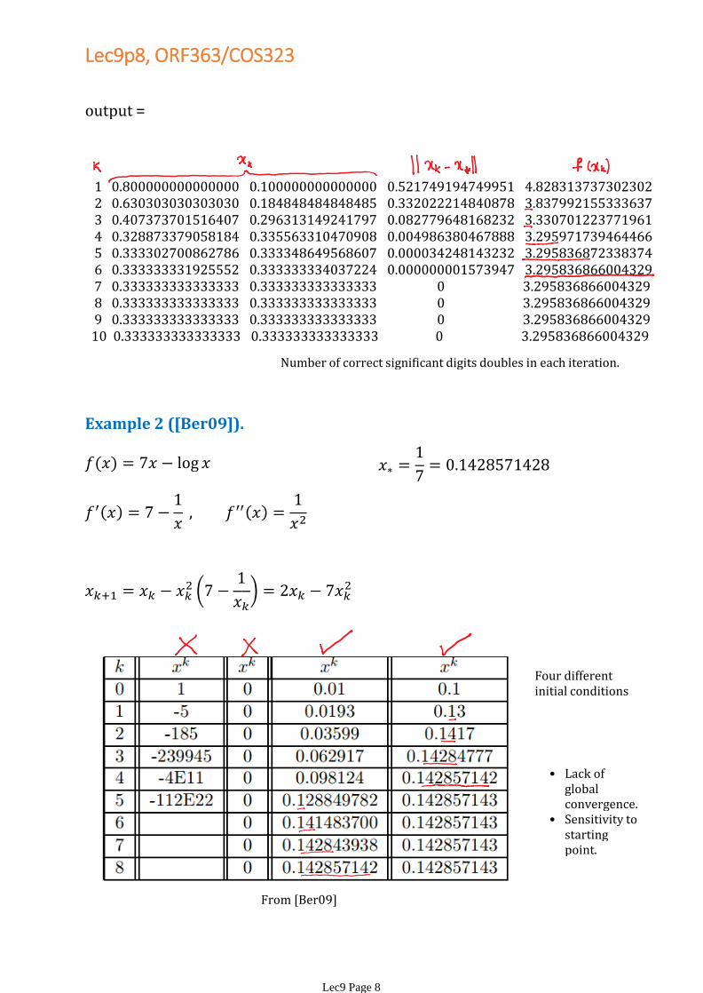
output =
1 0.800000000000000 0.100000000000000 0.521749194749951 4.828313737302302 2 0.630303030303030 0.184848484848485 0.332022214840878 3.837992155333637 3 0.407373701516407 0.296313149241797 0.082779648168232 3.330701223771961 4 0.328873379058184 0.335563310470908 0.004986380467888 3.295971739464466 5 0.333302700862786 0.333348649568607 0.000034248143232 3.295836872338374 6 0.333333331925552 0.333333334037224 0.000000001573947 3.295836866004329 7 0.333333333333333 0.333333333333333 0 3.295836866004329 8 0.333333333333333 0.333333333333333 0 3.295836866004329 9 0.333333333333333 0.333333333333333 0 3.295836866004329 10 0.333333333333333 0.333333333333333 0 3.295836866004329
Example 2 ([Ber09]).
From [Ber09]
Four different initial conditions
Number of correct significant digits doubles in each iteration.
Lack of global convergence.
•
Sensitivity to starting point.
•
Lec9p8, ORF363/COS323
Lec9 Page 8
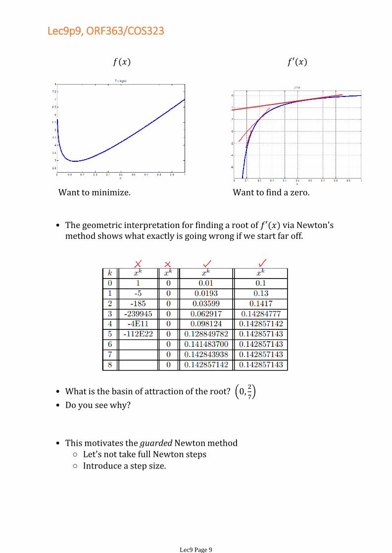
Want to minimize. Want to find a zero.
The geometric interpretation for finding a root of via Newton's method shows what exactly is going wrong if we start far off.
•
What is the basin of attraction of the root?
•
Do you see why?•
Let's not take full Newton steps○
Introduce a step size.○
This motivates the guarded Newton method•
Lec9p9, ORF363/COS323
Lec9 Page 9
Newton's method does not guarantee descent in every iteration; i.e., we may have
•
Means that if you make a small enough step, you do get the decrease property.
○
But the Newton direction is a descent direction for convex functions.•
Let's recall this notion and prove this statement formally.•
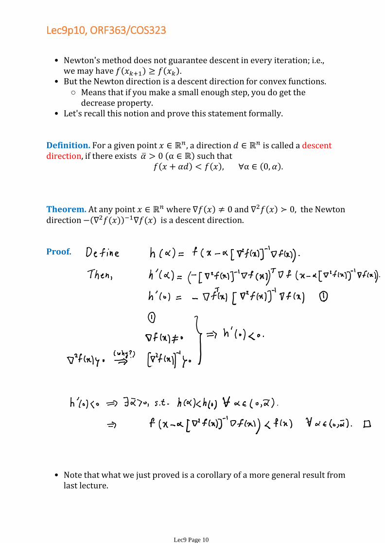
Definition. For a given point a direction is called a descent direction, if there exists such that
Theorem. At any point where and the Newton direction is a descent direction.
Proof.
Note that what we just proved is a corollary of a more general result from last lecture.
•
Lec9p10, ORF363/COS323
Lec9 Page 10
Newton method with a step size
We saw many choices of the step size in the previous lecture.•Let's learn about a new and a very popular one:•
The Armijo Rule
This is an inexact line search method. It does not find the exact minimum along the line. But it guarantees sufficient decrease and it's cheap.
•
Armijo rule requires two parameters: •
Suppose we would like to minimize a univariate function over (For us, where and are fixed and is a direction to go along, e.g., the Newton direction.)
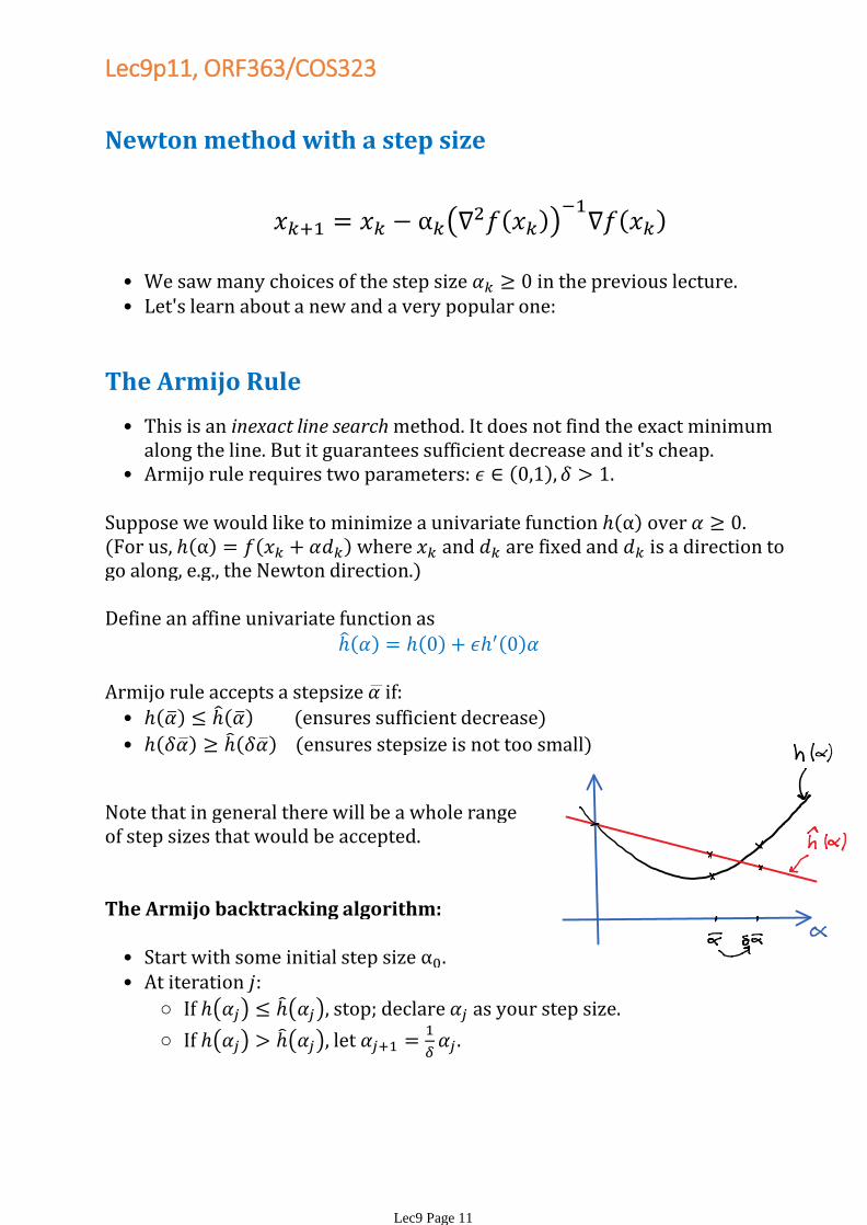
Define an affine univariate function as
(ensures sufficient decrease)•
(ensures stepsize is not too small)•
Armijo rule accepts a stepsize if:
Note that in general there will be a whole rangeof step sizes that would be accepted.
The Armijo backtracking algorithm:
Start with some initial step size •
If stop; declare as your step size.○
If let
○
At iteration •
Lec9p11, ORF363/COS323
Lec9 Page 11
Levenberg-Marquardt Modification
If Newton's direction may not be a descent direction.•If is singular, Newton's direction is not even well-defined.•Idea: let's make positive definite if it isn't.•
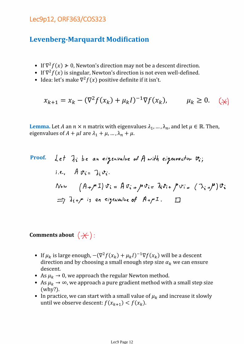
Lemma. Let an matrix with eigenvalues and let Then, eigenvalues of are
Proof.
Comments about
If is large enough, will be a descent
direction and by choosing a small enough step size we can ensure descent.
•
As we approach the regular Newton method.•As we approach a pure gradient method with a small step size (why?).
•
In practice, we can start with a small value of and increase it slowly until we observe descent:
•
Lec9p12, ORF363/COS323
Lec9 Page 12
The Gauss-Newton method for nonlinear least squares
time
Temp.
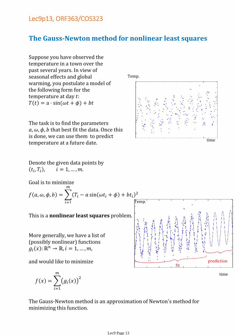
Suppose you have observed the temperature in a town over the past several years. In view of seasonal effects and global warming, you postulate a model of the following form for the temperature at day
The task is to find the parameters that best fit the data. Once this is done, we can use them to predict temperature at a future date.
Denote the given data points by
Goal is to minimize
This is a nonlinear least squares problem.
More generally, we have a list of (possibly nonlinear) functions
and would like to minimize
The Gauss-Newton method is an approximation of Newton's method for minimizing this function.
predictionfit
time
Temp.
Lec9p13, ORF363/COS323
Lec9 Page 13
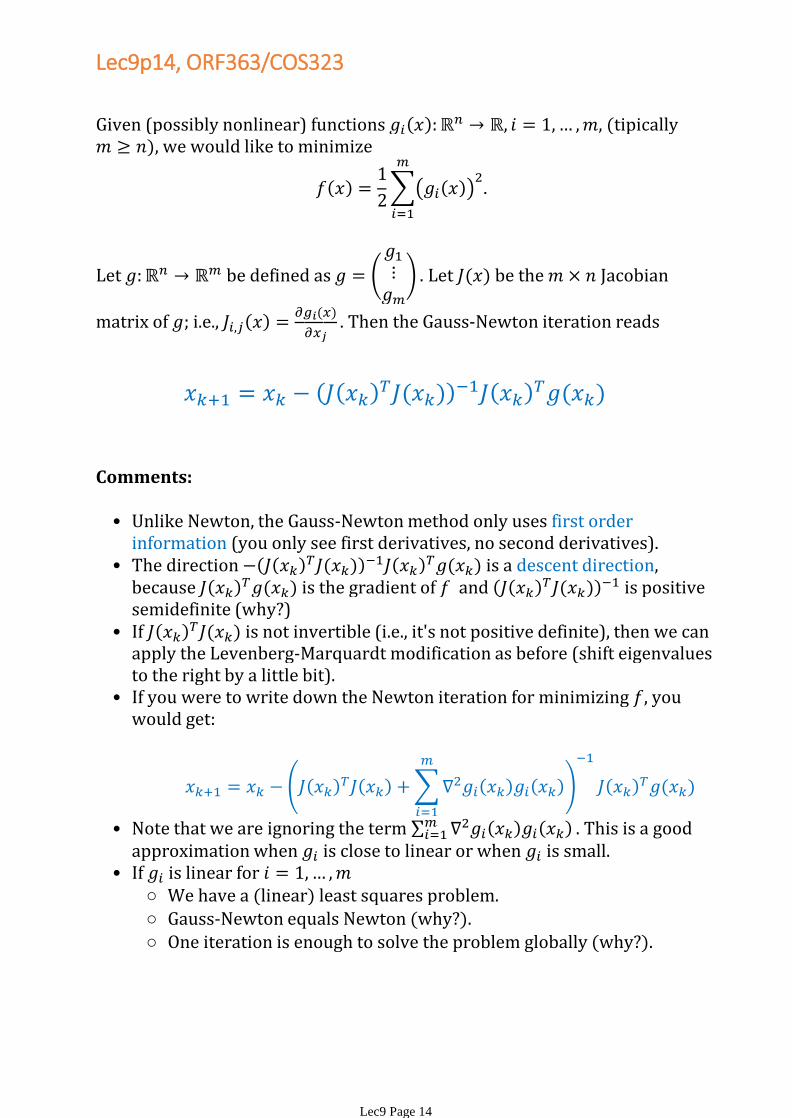
Given (possibly nonlinear) functions (tipically
), we would like to minimize
Let be defined as
Let be the Jacobian
matrix of i.e.,
Then the Gauss-Newton iteration reads
Comments:
Unlike Newton, the Gauss-Newton method only uses first order information (you only see first derivatives, no second derivatives).
•
The direction
is a descent direction,
because is the gradient of and
is positive
semidefinite (why?)
•
If is not invertible (i.e., it's not positive definite), then we can
apply the Levenberg-Marquardt modification as before (shift eigenvalues to the right by a little bit).
•
If you were to write down the Newton iteration for minimizing you would get:
•
Note that we are ignoring the term This is a good
approximation when is close to linear or when is small.•
We have a (linear) least squares problem.○
Gauss-Newton equals Newton (why?).○
One iteration is enough to solve the problem globally (why?).○
If is linear for •
Lec9p14, ORF363/COS323
Lec9 Page 14
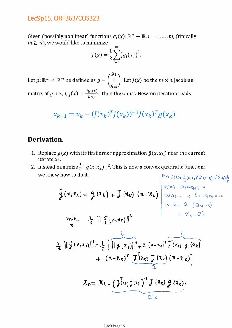
Given (possibly nonlinear) functions (tipically
), we would like to minimize
Let be defined as
Let be the Jacobian
matrix of i.e.,
Then the Gauss-Newton iteration reads
Derivation.
Replace with its first order approximation near the current iterate
1.
Instead minimize
This is now a convex quadratic function;
we know how to do it.
2.
Lec9p15, ORF363/COS323
Lec9 Page 15
Notes:The relevant [CZ13]chapter for this lecture is Chapter 9.
References:
[Bert09] D. Bertsimas. Lecture notes on optimization methods (6.255). MIT OpenCourseWare, 2009.
-
[Bert03] D.P. Bertsekas. Nonlinear Programming.Second edition. Athena Scientific, 2003.
-
[CZ13] E.K.P. Chong and S.H. Zak. An Introduction to Optimization. Fourth edition. Wiley, 2013.
-
[Tit13] A.L. Tits. Lecture notes on optimal control. University of Maryland, 2013.
-
Lec9p16, ORF363/COS323
Lec9 Page 16
![Lec3p1, ORF363/COS323 · See, e.g., Theorem 3.7 in Section 3.4 of [CZ13]. Examples: MATLAB: eig([2 4;4 5]) Recall our easy test in dimension 2: This generalizes to n dimensions using](https://img.pdfslide.us/doc/110x75/5fbe7126b9248435bd3cb438/lec3p1-orf363-see-eg-theorem-37-in-section-34-of-cz13-examples-matlab.jpg)


![Lec8p1, ORF363/COS323 - Princeton Universityand Goldstein rule (see, e.g., Section 7.8 of [CZ13]). We will cover Armijo in the next lecture. • Try to ensure enough decrease in line](https://img.pdfslide.us/doc/110x75/5ea70631682dc05c89134fc2/lec8p1-orf363cos323-princeton-and-goldstein-rule-see-eg-section-78-of.jpg)