Embed Size (px)
Citation preview
Email: [email protected] Phone:0851397780 1
Leaving Certificate Higher Level Mathematics - STATISTICS SECTION
Paper 2 Layout of Paper 2:
Section A: 150 marks (usually 6 short questions)
Section B: 150 marks (can feature 2,3 or 4 questions)
Timing:
Section A generally contains easier skills based questions. It is very important to remember that section A contains
the same marks as section B, so each section should be given approx half of the time.
In general section A contains 6 questions worth 25 marks each. You should aim to spend no more than 12 minutes
on any of these questions. It is very important that you work on your timing and don't end up spending more than 12
minutes on a part (c) of these questions. If a question is poorly answered across the country the marking scheme will
be changed to reflect this and you are losing time that can gain you marks on other questions.
SO THE RECOMMENDED APPROACH IS TO TAKE CARE AND PICK UP ALL MARKS ON THE EASY STUFF, AND IF
SOMETHING SEEMS DIFFICULT, AT LEAST HAVE A GO AT IT. "ATTEMPT" MARKS CAN CONTRIBUTE A LOT TO YOUR
GRADE!
EXAM TIPS:
1. Start by briefly reading through the paper as this allows you to subconsciously think about future questions. If you
like you can jot down some short notes as you go. DON'T SPEND MORE THAN 10 MINUTES DOING THIS.
2. It is a good idea to start with your favourite question to settle any nerves.
3. Then you work through the paper tracking your time as you go. DON’T GET BOGGED DOWN OR LOSE TRACK OF
TIME.
4. Read each question more than once highlighting any important information for finishing the question e.g. write
your answer to three significant figures or find the coordinates. These are simple marks that can be lost at the end of
questions completed correctly .
5. Show all workings - if you solve a problem using your calculator write out some or all of the steps taken.
6. NEVER EVER leave a blank answer - THE ONLY REALLY "STUPID" ANSWER IS A BLANK ANSWER! "Attempt" marks
can add up to better grades!
7. Before leaving a question make sure you have answered everything required.
Topics to be revised for paper 1:
1. The Line
2. The Circle
3. Geometry (including Enlargements)
4. Trigonometry
5. Probability
6. Statistics
THESE TOPICS HAVE ALL APPEARED ON PAPER 2, HOWEVER THIS DOES NOT MEAN THAT TOPICS FROM PAPER 1
WILL NOT APPEAR ON THIS PAPER AND VISA VERSA. For example, you will see Algebra everywhere in Paper 2 as it is
required for most topics.
Email: [email protected] Phone:0851397780 2
Statistics Before we get into representing and analysing data we must first look at the theory and importance
associated with selecting a sample from a population in order to actually carry out a survey. On the LC HL
course there are a number of key terms that we must be familiar with for the exam as these terms can
appear in the exam or we could even be asked the definitions for some. These key terms are listed below.
Definitions & Sampling: A population is the entire group being studied.
A sample is a smaller group from within the population.
A census is a survey of the entire population.
N.B. You can be asked to distinguish between the next two definitions in a question in the exam. Since you did not
study Inferential Statistics at JC this is the first time that you will have dealt with a parameter so it is crucial that you
know what it means if it appears in the exam.
A statistic is a numerical measurement of some characteristic of a sample. For example, the mean age of a sample of
10 teachers from Pipers Hill. This statistic would change given a different sample.
A parameter is a numerical measurement of some characteristic of the population. It is a fixed number but we
probably don’t know it’s value (since the entire population is much larger).
Biased Samples are samples that are not representative of the whole population. They tend to overestimate or
underestimate the parameter of interest.
Random sampling is where everyone must have an equal chance of being selected. This leads us to Simple Random
Sampling next.
Simple Random Sampling is a random sample where every member of the population is equally likely to be selected.
It can be achieved in the following way:
Imagine I wanted to select 30 people from a group of people on an aeroplane. I want to choose 30 people at random.
I could pick names out of a hat
I could select random seat numbers – how??
Both of these ways, everyone has an equal chance of being selected with anyone else on the plane.
So in an SRS everyone must have an equal chance of being selected with everyone else.
N.B.You can be asked to define any or all of the next definitions in a question in the exam. It is simply crucial that
you learn these definitions off by heart.
Stratified Random Sampling is where the population is first divided into subgroups so that individuals within each
subgroup share characteristics. Then a random sample is drawn from each group to form the full sample.(E.g. We
might first divide population by gender).
Cluster Sampling is where the population is divided by sections or clusters. Then some of those clusters are randomly
selected and all members from those clusters are chose. (E.g. We want a sample of students. We get a list of schools
and then select a school and use those students).
Quota sampling is non – probability sampling. We select to fill a quota of a certain type of subgroup. (E.g. Certain
type of subgroup could be men over 50. The person selecting the sample does so in the most convenient way
possible. Randomisation does not play a role in selection process so therefore this method is open to mistakes).
Email: [email protected] Phone:0851397780 4
Recognise what an outlier in a data set is and understand the effect it has on a data set. Outliers are extreme values that are not typical of the other values in the data set. For example look at a date set of
{8, 7 , 8 , 9 ,11, 12, 81, 12}. 81 is an outlier here because it is so far away from the other numbers in the data set.
It is of utmost importance that we can not only recognise what an outlier is but actually realise the effect it has on
the mean of a data set.
To see this effect let’s first calculate mean of the set above, WITHOUT the outlier included.
MEAN =
Now let’s calculate the mean of the set above, WITH the outlier included.
MEAN =
It is quite clear to see that an outlier has an effect on the mean (average) of a data set. Here, the large outlier has
increased the size of the mean.
Similarly, a small outlier will reduce the value of the mean.
However, outliers will have no effect on the median or mode of a data set. We see this in the table above
In relation to the spread/variability of data, outliers will again have an effect. See below for this and pay particular
attention to the diagrams for symmetric and skewed distribution to again see the effect that the outlier has on a
data set.
Analysing and Observing the shape of a graph There are three shapes of distributions:
Symmetric
Skewed left (negatively skewed)
Skewed Right (positively skewed)
The three measures of shape are: Symmetric, skewed right and skewed left (you will only be asked about these on
a histogram, stem – and- leaf or a bar chart)
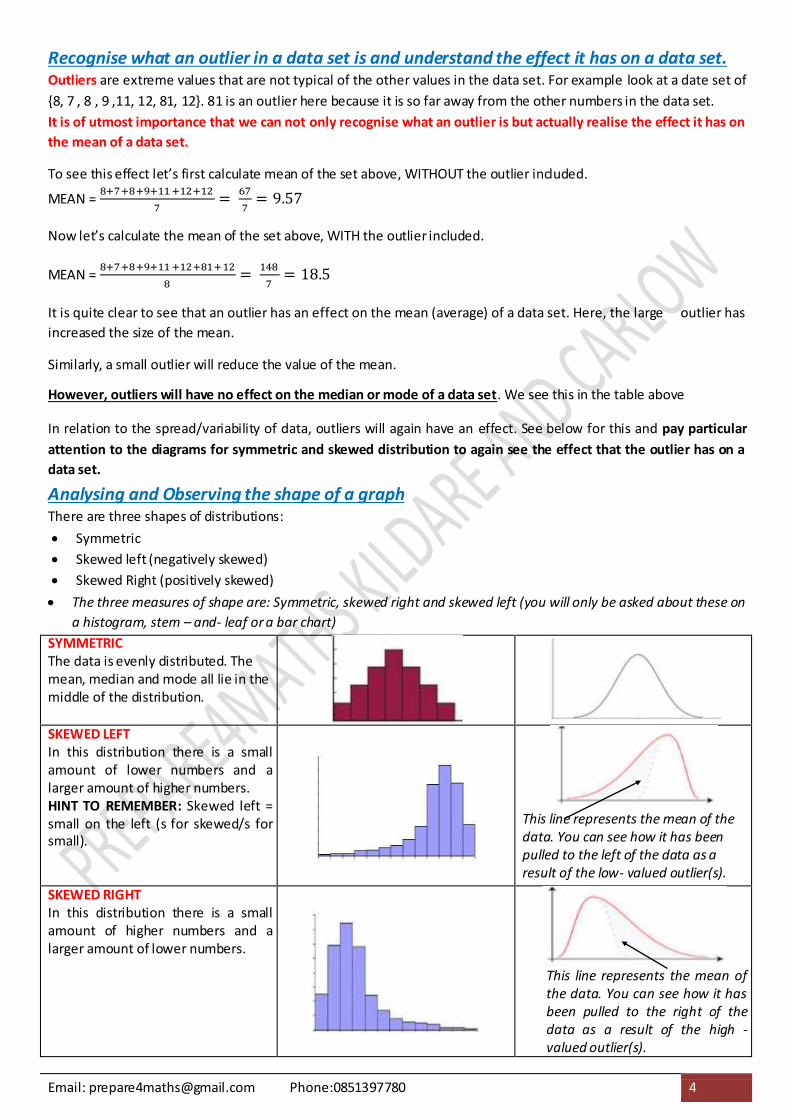
SYMMETRIC The data is evenly distributed. The mean, median and mode all lie in the middle of the distribution. SKEWED LEFT In this distribution there is a small amount of lower numbers and a larger amount of higher numbers. HINT TO REMEMBER: Skewed left = small on the left (s for skewed/s for small).
This line represents the mean of the data. You can see how it has been pulled to the left of the data as a result of the low- valued outlier(s).
SKEWED RIGHT In this distribution there is a small amount of higher numbers and a larger amount of lower numbers.
This line represents the mean of the data. You can see how it has been pulled to the right of the data as a result of the high - valued outlier(s).
Email: [email protected] Phone:0851397780 6
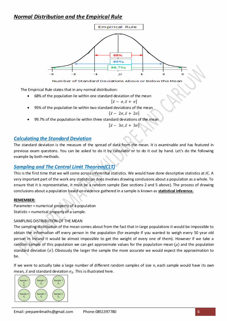
Normal Distribution and the Empirical Rule
The Empirical Rule states that in any normal distribution:
68% of the population lie within one standard deviation of the mean
95% of the population lie within two standard deviations of the mean
99.7% of the population lie within three standard deviations of the mean
Calculating the Standard Deviation
The standard deviation is the measure of the spread of data from the mean. It is examinable and has featured in
previous exam questions. You can be asked to do it by calculator or to do it out by hand. Let’s do the following
example by both methods.
Sampling and The Central Limit Theorem(CLT) This is the first time that we will come across inferential statistics. We would have done descriptive statistics at JC. A
very important part of the work any statistician does involves drawing conclusions about a population as a whole. To
ensure that it is representative, it must be a random sample (See sections 2 and 5 above). The process of drawing
conclusions about a population based on evidence gathered in a sample is known as statistical inference.
REMEMBER:
Parameter = numerical property of a population
Statistic = numerical property of a sample.
SAMPLING DISTRIBUTION OF THE MEAN
The sampling distribution of the mean comes about from the fact that in large populations it would be impossible to
obtain the information off every person in the population (for example if you wanted to weigh every 50 year old
person in Ireland it would be almost impossible to get the weight of every one of them). However if we take a
random sample of this population we can get approximate values for the population mean and the population
standard deviation Obviously the larger the sample the more accurate we would expect the approximation to
be.
If we were to actually take a large number of different random samples of size each sample would have its own
mean, and standard deviation . This is illustrated here.
Email: [email protected] Phone:0851397780 7
The different means of these samples are called the sample means.
Obviously if we were to take a large number of samples of the same size, then we would have a large number of
sample means. These means form their own distribution giving us the distribution of the sample means.
This distribution is called the sampling distribution of the mean.
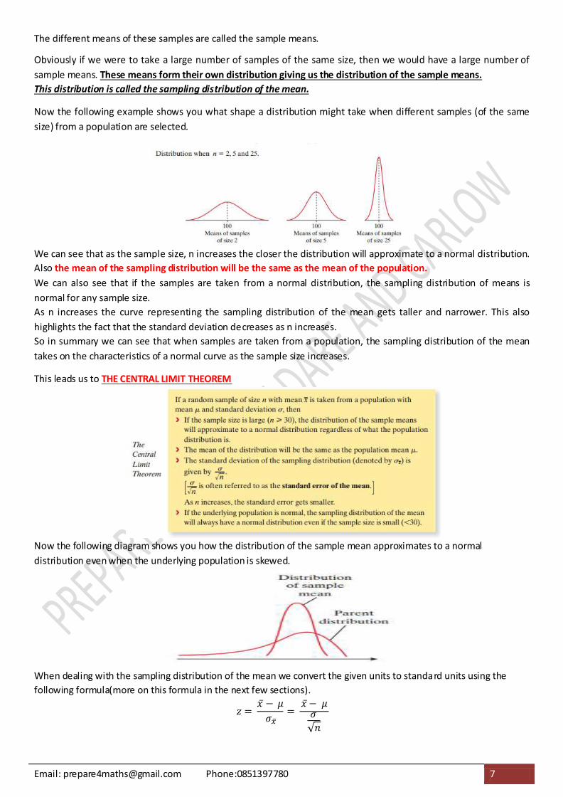
Now the following example shows you what shape a distribution might take when different samples (of the same
size) from a population are selected.
We can see that as the sample size, n increases the closer the distribution will approximate to a normal distribution.
Also the mean of the sampling distribution will be the same as the mean of the population.
We can also see that if the samples are taken from a normal distribution, the sampling distribution of means is
normal for any sample size.
As n increases the curve representing the sampling distribution of the mean gets taller and narrower. This also
highlights the fact that the standard deviation decreases as n increases.
So in summary we can see that when samples are taken from a population, the sampling distribution of the mean
takes on the characteristics of a normal curve as the sample size increases.
This leads us to THE CENTRAL LIMIT THEOREM
Now the following diagram shows you how the distribution of the sample mean approximates to a normal
distribution even when the underlying population is skewed.
When dealing with the sampling distribution of the mean we convert the given units to standard units using the
following formula(more on this formula in the next few sections).
Email: [email protected] Phone:0851397780 9
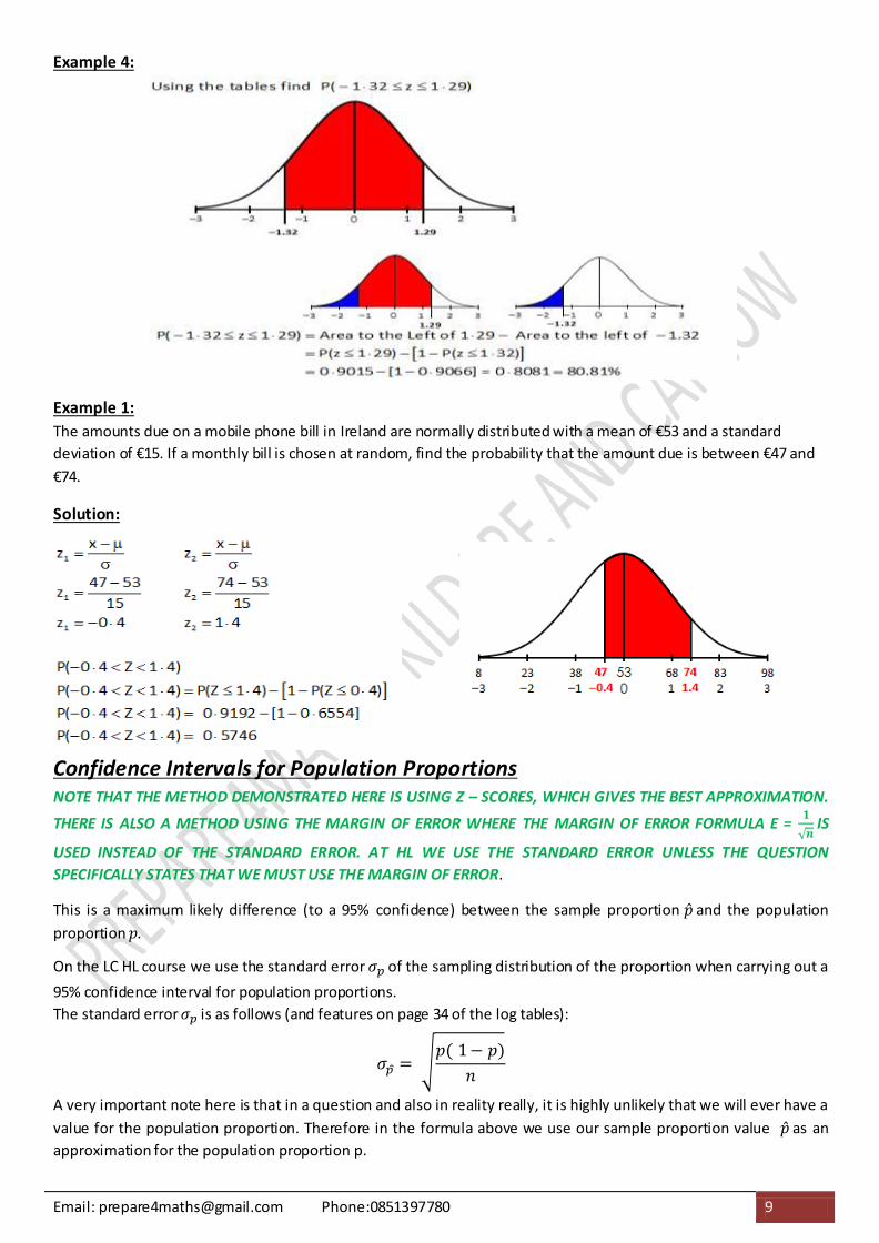
Example 4:
Example 1:
The amounts due on a mobile phone bill in Ireland are normally distributed with a mean of €53 and a standard
deviation of €15. If a monthly bill is chosen at random, find the probability that the amount due is between €47 and
€74.
Solution:
Confidence Intervals for Population Proportions
NOTE THAT THE METHOD DEMONSTRATED HERE IS USING Z – SCORES, WHICH GIVES THE BEST APPROXIMATION.
THERE IS ALSO A METHOD USING THE MARGIN OF ERROR WHERE THE MARGIN OF ERROR FORMULA E =
IS
USED INSTEAD OF THE STANDARD ERROR. AT HL WE USE THE STANDARD ERROR UNLESS THE QUESTION
SPECIFICALLY STATES THAT WE MUST USE THE MARGIN OF ERROR.
This is a maximum likely difference (to a 95% confidence) between the sample proportion and the population
proportion
On the LC HL course we use the standard error of the sampling distribution of the proportion when carrying out a
95% confidence interval for population proportions.
The standard error is as follows (and features on page 34 of the log tables):
A very important note here is that in a question and also in reality really, it is highly unlikely that we will ever have a
value for the population proportion. Therefore in the formula above we use our sample proportion value as an
approximation for the population proportion p.
Email: [email protected] Phone:0851397780 10
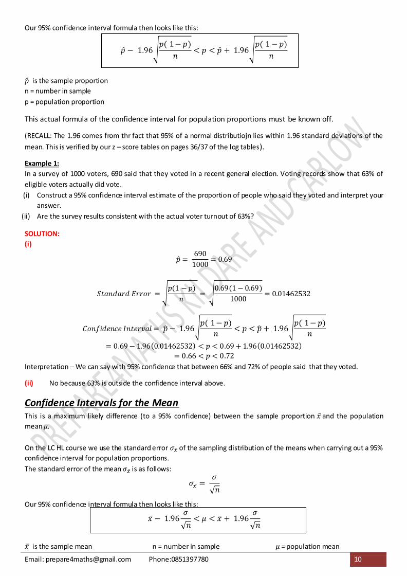
Our 95% confidence interval formula then looks like this:
is the sample proportion
n = number in sample
p = population proportion
This actual formula of the confidence interval for population proportions must be known off.
(RECALL: The 1.96 comes from thr fact that 95% of a normal distributiojn lies within 1.96 standard deviations of the
mean. This is verified by our z – score tables on pages 36/37 of the log tables).
Example 1:
In a survey of 1000 voters, 690 said that they voted in a recent general election. Voting records show that 63% of
eligible voters actually did vote.
(i) Construct a 95% confidence interval estimate of the proportion of people who said they voted and interpret your
answer.
(ii) Are the survey results consistent with the actual voter turnout of 63%?
SOLUTION:
(i)
Interpretation – We can say with 95% confidence that between 66% and 72% of people said that they voted.
(ii) No because 63% is outside the confidence interval above.
Confidence Intervals for the Mean
This is a maximum likely difference (to a 95% confidence) between the sample proportion and the population
mean
On the LC HL course we use the standard error of the sampling distribution of the means when carrying out a 95%
confidence interval for population proportions.
The standard error of the mean is as follows:
Our 95% confidence interval formula then looks like this:
is the sample mean n = number in sample = population mean
Email: [email protected] Phone:0851397780 11
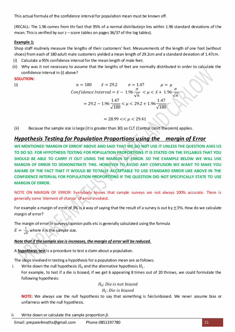
This actual formula of the confidence interval for population mean must be known off.
(RECALL: The 1.96 comes from thr fact that 95% of a normal distributiojn lies within 1.96 standard deviations of the
mean. This is verified by our z – score tables on pages 36/37 of the log tables).
Example 1:
Shop staff routinely measure the lengths of their customers’ feet. Measurements of the length of one foot (without
shoes) from each of 180 adult male customers yielded a mean length of 29.2cm and a standard deviation of 1.47cm.
(i) Calculate a 95% confidence interval for the mean length of male feet.
(ii) Why was it not necessary to assume that the lengths of feet are normally distributed in order to calculate the
confidence interval in (i) above?
SOLUTION:
(i)
(ii) Because the sample size is large (it is greater than 30) so CLT (Central Limit Theorem) applies.
Hypothesis Testing for Population Proportions using the margin of Error
WE MENTIONED ‘MARGIN OF ERROR’ ABOVE AND SAID THAT WE DO NOT USE IT UNLESS THE QUESTION ASKS US
TO DO SO. FOR HYPOTHESIS TESTING FOR POPULATION PROPORTIONS IT IS STATED ON THE SYLLABUS THAT YOU
SHOULD BE ABLE TO CARRY IT OUT USING THE MARGIN OF ERROR. SO THE EXAMPLE BELOW WE WILL USE
MARGIN OF ERROR TO DEMONSTRATE THIS. HOWEVER TO AVOID ANY CONFUSION WE WANT TO MAKE YOU
AWARE OF THE FACT THAT IT WOULD BE TOTALLY ACCEPTABLE TO USE STANDARD ERROR LIKE ABOVE IN THE
CONFIDENCE INTERVAL FOR POPULATION PROPORTIONS IF THE QUESTION DID NOT SPECIFICALLY STATE TO USE
MARGIN OF ERROR.
NOTE ON MARGIN OF ERROR: Everybody knows that sample surveys are not always 100% accurate. There is
generally some ‘element of chance’ of error involved.
For example a margin of error of 3% is a way of saying that the result of a survey is out by How do we calculate
margin of error?
The margin of error in surveys/opinion polls etc is generally calculated using the formula
where n is the sample size.
Note that if the sample size is increases, the margin of error will be reduced.
A hypothesis test is a procedure to test a claim about a population.
The steps involved in testing a hypothesis for a population mean are as follows:
i. Write down the null hypothesis and the alternative hypothesis
For example, to test if a die is biased, if we get 6 appearing 8 times out of 20 throws, we could formulate the
following hypothesis:
NOTE: We always use the null hypothesis to say that something is fair/unbiased. We never assume bias or
unfairness with the null hypothesis.
ii. Write down or calculate the sample proportion