Least-Squares Regression---Prediction, Outliers,

Influential Points and Extrapolation

• Section 3.3----Part IISection 3.3----Part II

What You’ll Learn:

• How to use the LSRL for predictionHow to use the LSRL for prediction• Why we need to be cautious when Why we need to be cautious when

predicting outside our original datapredicting outside our original data• How to spot an “outlier”How to spot an “outlier”• The effect of an “influential point”The effect of an “influential point”

Using the LSRL for predictionUsing the LSRL for predictionOnce we have determined we have a useful Once we have determined we have a useful

model, we tend to use the model for model, we tend to use the model for prediction.prediction.

Let’s consider a new set of data:Let’s consider a new set of data:The following is the distance (in miles) as The following is the distance (in miles) as

well as the airfare for twelve destinations well as the airfare for twelve destinations from Baltimore Maryland. A scatterplot from Baltimore Maryland. A scatterplot

is included. is included.

Traveling from BaltimoreCollection 1

=

City Distance Airfare <new>

1

2

3

4

5

6

7

8

9

10

11

12

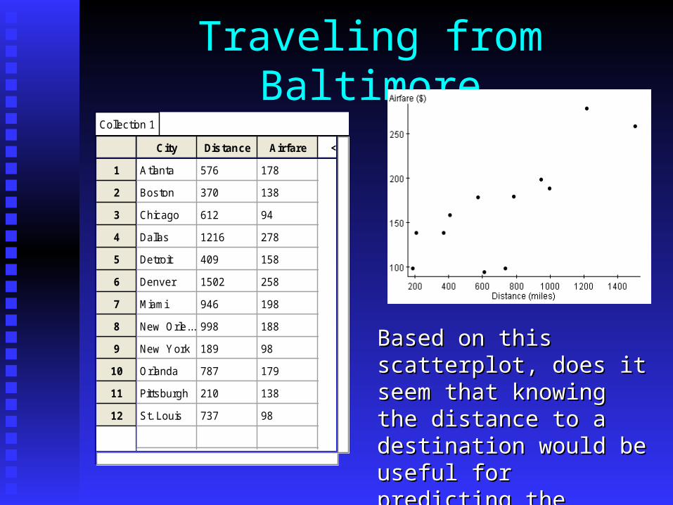
Atlanta 576 178

Boston 370 138

Chicago 612 94

Dallas 1216 278

Detroit 409 158

Denver 1502 258

Miami 946 198

New Orle... 998 188

New York 189 98

Orlanda 787 179

Pittsburgh 210 138

St. Louis 737 98

Based on this Based on this scatterplot, does it scatterplot, does it seem that knowing the seem that knowing the distance to a distance to a destination would be destination would be useful for predicting the useful for predicting the airfare?airfare?

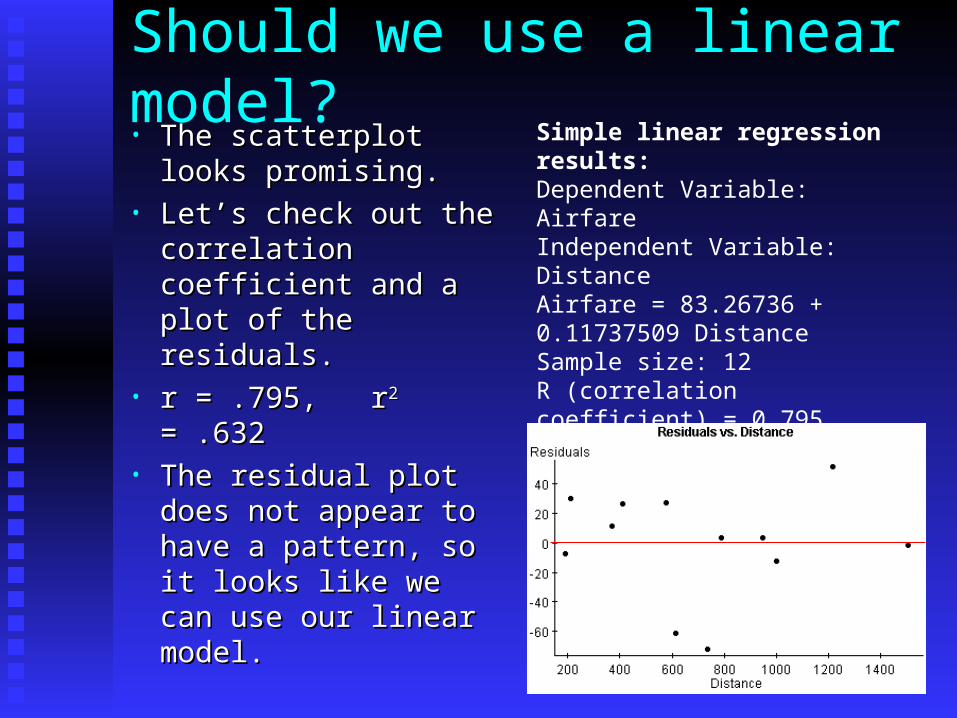
Should we use a linear model?• The scatterplot The scatterplot

looks promising.looks promising.• Let’s check out the Let’s check out the

correlation correlation coefficient and a coefficient and a plot of the residuals.plot of the residuals.

• r = .795, rr = .795, r22 = .632 = .632• The residual plot The residual plot

does not appear to does not appear to have a pattern, so it have a pattern, so it looks like we can looks like we can use our linear use our linear model.model.

Simple linear regression results: Dependent Variable: Airfare Independent Variable: Distance Airfare = 83.26736 + 0.11737509 Distance Sample size: 12 R (correlation coefficient) = 0.795 R-sq = 0.63200194 Estimate of error standard deviation: 37.827023

Using the model for prediction

• LSRL for Distance vs AirfareLSRL for Distance vs Airfare• Airfare = 83.26736 + 0.11737509( Distance)Airfare = 83.26736 + 0.11737509( Distance)

• When we use our regression equation for prediction, When we use our regression equation for prediction, remember we are finding the “average” response value for remember we are finding the “average” response value for a particular explanatory value.a particular explanatory value.

• This means that our predicted values will not always agree This means that our predicted values will not always agree with actual observed values. We will under-predict for with actual observed values. We will under-predict for some and over-predict for others.some and over-predict for others.

• To see this in action, let’s consider predicting for one of To see this in action, let’s consider predicting for one of the distances we used to compute the LSRLthe distances we used to compute the LSRL

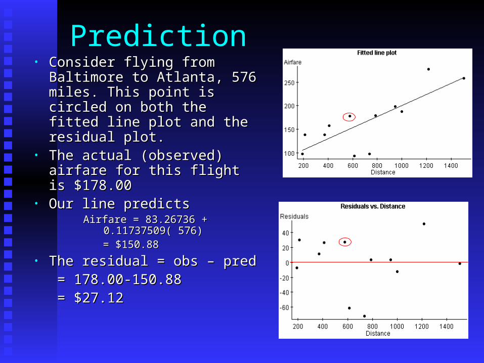
Prediction• Consider flying from Baltimore Consider flying from Baltimore

to Atlanta, 576 miles. This to Atlanta, 576 miles. This point is circled on both the point is circled on both the fitted line plot and the residual fitted line plot and the residual plot.plot.

• The actual (observed) airfare The actual (observed) airfare for this flight is $178.00for this flight is $178.00

• Our line predictsOur line predictsAirfare = 83.26736 + 0.11737509( 576)Airfare = 83.26736 + 0.11737509( 576) = $150.88= $150.88

• The residual = obs – predThe residual = obs – pred = 178.00-= 178.00-

150.88150.88 = $27.12= $27.12

Prediction

• Notice these three things:Notice these three things:• The actual point is The actual point is aboveabove the fitted line the fitted line• The residual is The residual is aboveabove the “zero” line the “zero” line• The value of the residual is positiveThe value of the residual is positive

• All these indicate that our prediction line All these indicate that our prediction line will will under-predictunder-predict for this particular airfare for this particular airfare

Over and Under Predictions

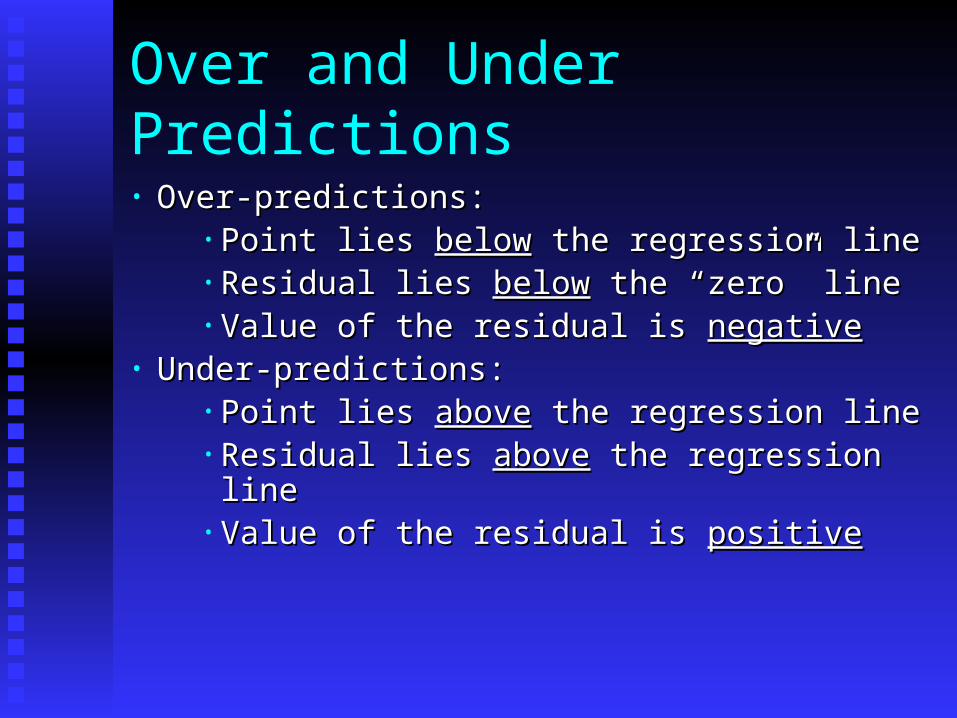
• Over-predictions:Over-predictions:• Point lies Point lies belowbelow the regression line the regression line• Residual lies Residual lies belowbelow the “zero” line the “zero” line• Value of the residual is Value of the residual is negativenegative

• Under-predictions:Under-predictions:• Point lies Point lies aboveabove the regression line the regression line• Residual lies Residual lies aboveabove the regression line the regression line• Value of the residual is Value of the residual is positivepositive

Prediction Errors

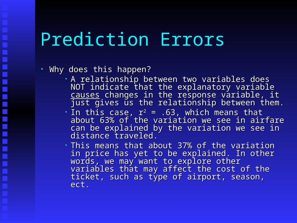
• Why does this happen? Why does this happen? • A relationship between two variables does NOT A relationship between two variables does NOT

indicate that the explanatory variable indicate that the explanatory variable causescauses changes in the response variable, it just gives us the changes in the response variable, it just gives us the relationship between them.relationship between them.

• In this case, rIn this case, r22 = .63, which means that about 63% of = .63, which means that about 63% of the variation we see in airfare can be explained by the variation we see in airfare can be explained by the variation we see in distance traveled.the variation we see in distance traveled.

• This means that about 37% of the variation in price This means that about 37% of the variation in price has yet to be explained. In other words, we may has yet to be explained. In other words, we may want to explore other variables that may affect the want to explore other variables that may affect the cost of the ticket, such as type of airport, season, cost of the ticket, such as type of airport, season, ect.ect.

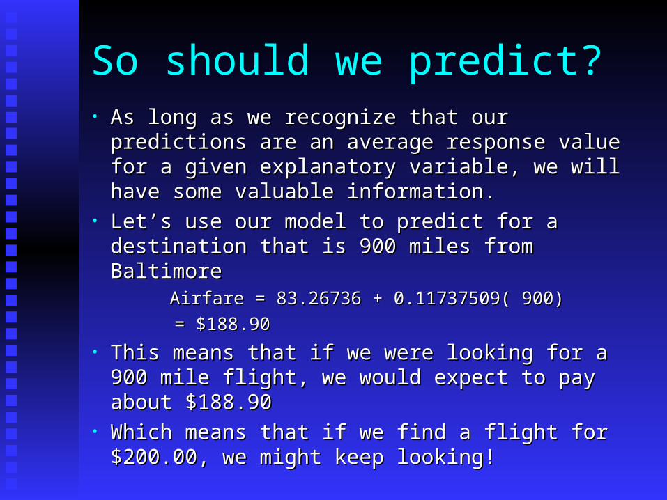
So should we predict?• As long as we recognize that our predictions are As long as we recognize that our predictions are

an average response value for a given explanatory an average response value for a given explanatory variable, we will have some valuable information.variable, we will have some valuable information.

• Let’s use our model to predict for a destination Let’s use our model to predict for a destination that is 900 miles from Baltimorethat is 900 miles from Baltimore

Airfare = 83.26736 + 0.11737509( 900)Airfare = 83.26736 + 0.11737509( 900)

= $188.90= $188.90

• This means that if we were looking for a 900 mile This means that if we were looking for a 900 mile flight, we would expect to pay about $188.90flight, we would expect to pay about $188.90

• Which means that if we find a flight for $200.00, Which means that if we find a flight for $200.00, we might keep looking!we might keep looking!

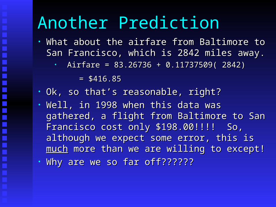
Another Prediction• What about the airfare from Baltimore to San What about the airfare from Baltimore to San

Francisco, which is 2842 miles away.Francisco, which is 2842 miles away.• Airfare = 83.26736 + 0.11737509( 2842)Airfare = 83.26736 + 0.11737509( 2842)

= $416.85= $416.85

• Ok, so that’s reasonable, right?Ok, so that’s reasonable, right?• Well, in 1998 when this data was gathered, a flight Well, in 1998 when this data was gathered, a flight

from Baltimore to San Francisco cost only from Baltimore to San Francisco cost only $198.00!!!! So, although we expect some error, $198.00!!!! So, although we expect some error, this is this is muchmuch more than we are willing to except! more than we are willing to except!

• Why are we so far off?????? Why are we so far off??????

Predicting outside our data• Consider the distances we used to create the model. They Consider the distances we used to create the model. They

range from New York at 189 miles to Denver, 1502 miles.range from New York at 189 miles to Denver, 1502 miles.

Collection 1

=

City Distance Airfare <new>

1

2

3

4

5

6

7

8

9

10

11

12

Atlanta 576 178

Boston 370 138

Chicago 612 94

Dallas 1216 278

Detroit 409 158

Denver 1502 258

Miami 946 198

New Orle... 998 188

New York 189 98

Orlanda 787 179

Pittsburgh 210 138

St. Louis 737 98

Our prediction for the flight to San Francisco assumes that the same relationship continues even though this distance is almost twice as far as Denver. We have no way of knowing if this relationship stays the same outside the domain of the original data. Predictions outside this domain is called “extrapolation”. This type of prediction is dangerous and should not be done.

Unusual Points (Outliers & Influential Points)

• Outliers are pieces of data that do not fit the Outliers are pieces of data that do not fit the overall pattern.overall pattern.

• If a point lies far away from the regression If a point lies far away from the regression line in the y-direction, it will have a large line in the y-direction, it will have a large residual (either positive or negative)residual (either positive or negative)

• Consider the following data which shows Consider the following data which shows the relationship between the age (in the relationship between the age (in months) at which a child first speaks and months) at which a child first speaks and their subsequent score on a test for mental their subsequent score on a test for mental ability—Gesell scoreability—Gesell score

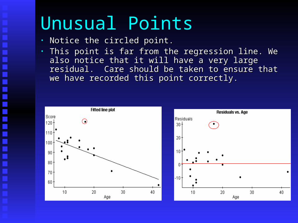
Unusual Points• Notice the circled point.Notice the circled point.• This point is far from the regression line. We also notice This point is far from the regression line. We also notice

that it will have a very large residual. Care should be that it will have a very large residual. Care should be taken to ensure that we have recorded this point correctly.taken to ensure that we have recorded this point correctly.

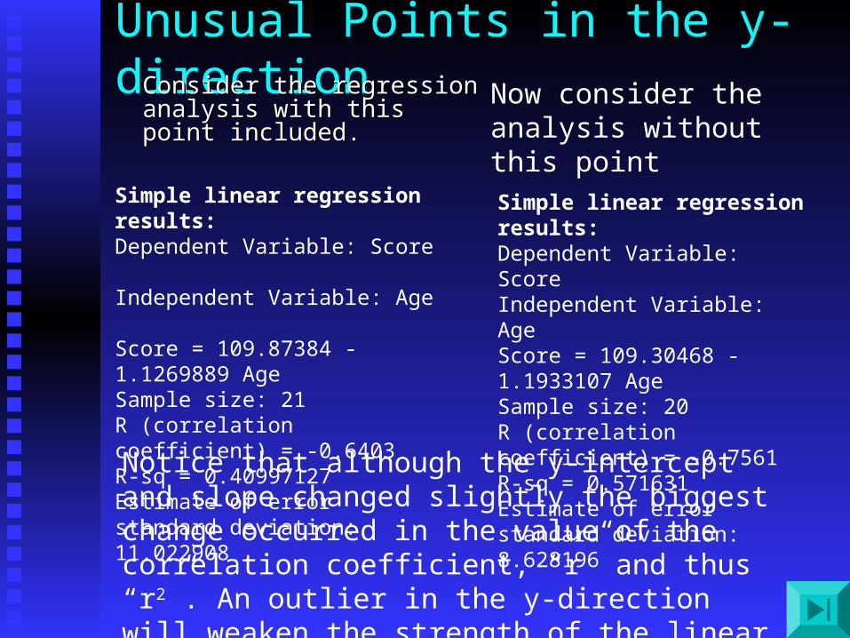
Unusual Points in the y-direction• Consider the regression Consider the regression

analysis with this point analysis with this point included. included.

Simple linear regression results: Dependent Variable: Score Independent Variable: Age Score = 109.87384 - 1.1269889 Age Sample size: 21 R (correlation coefficient) = -0.6403 R-sq = 0.40997127 Estimate of error standard deviation: 11.022908

Now consider the analysis without this point

Simple linear regression results: Dependent Variable: Score Independent Variable: Age Score = 109.30468 - 1.1933107 Age Sample size: 20 R (correlation coefficient) = -0.7561

R-sq = 0.571631 Estimate of error standard deviation: 8.628196

Notice that although the y-intercept and slope changed slightly the biggest change occurred in the value of the correlation coefficient, “r” and thus “r2”. An outlier in the y-direction will weaken the strength of the linear relationship

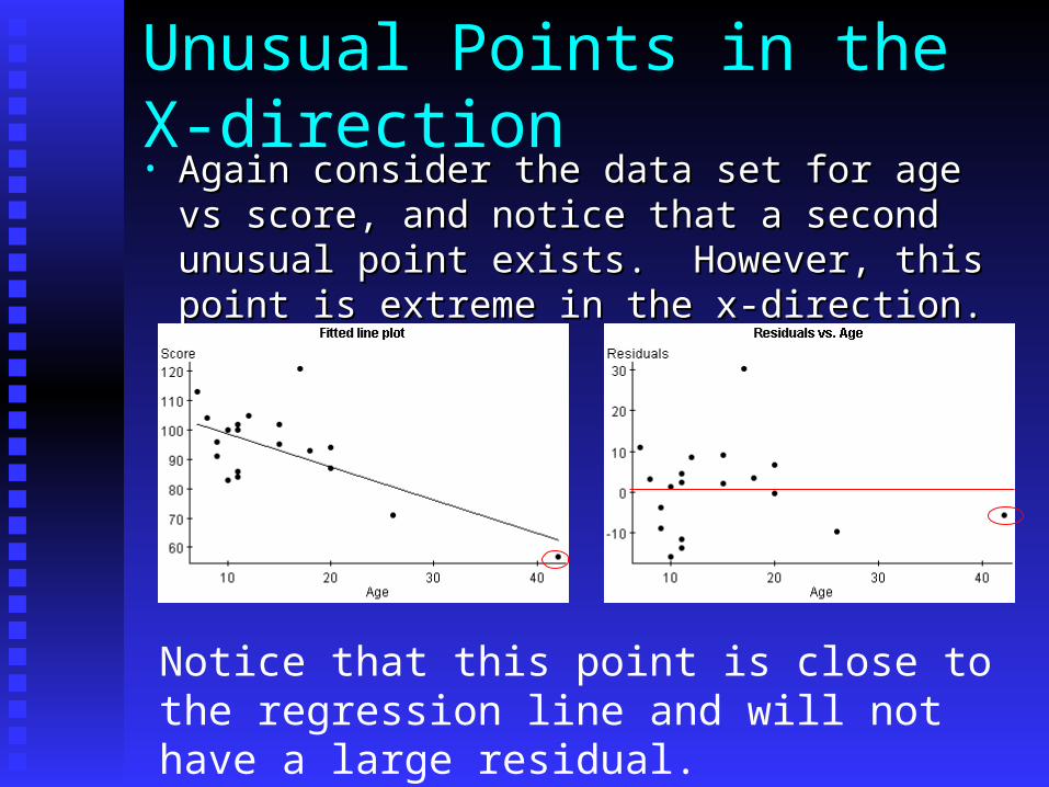
Unusual Points in the X-direction• Again consider the data set for age vs score, and Again consider the data set for age vs score, and

notice that a second unusual point exists. notice that a second unusual point exists. However, this point is extreme in the x-direction.However, this point is extreme in the x-direction.

Notice that this point is close to the regression line and will not have a large residual.

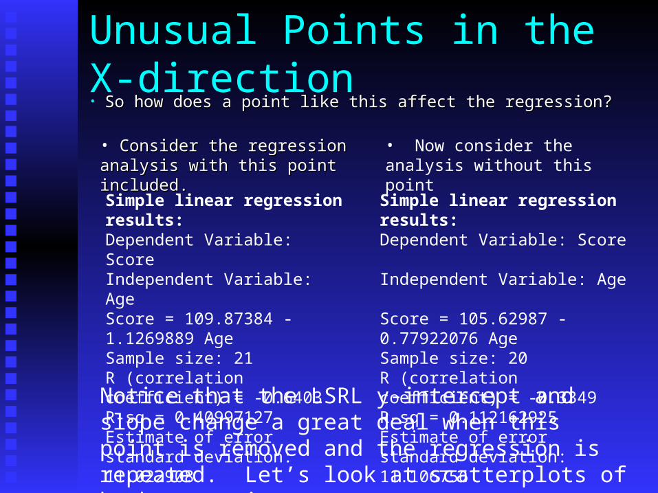
Unusual Points in the X-direction• So how does a point like this affect the regression?So how does a point like this affect the regression?

• Consider the regression analysis Consider the regression analysis with this point included.with this point included.

Simple linear regression results: Dependent Variable: Score Independent Variable: Age Score = 109.87384 - 1.1269889 Age Sample size: 21 R (correlation coefficient) = -0.6403

R-sq = 0.40997127 Estimate of error standard deviation: 11.022908

• Now consider the analysis without this point

Simple linear regression results: Dependent Variable: Score Independent Variable: Age Score = 105.62987 - 0.77922076 Age Sample size: 20 R (correlation coefficient) = -0.3349 R-sq = 0.112162925 Estimate of error standard deviation: 11.106756

Notice that the LSRL y-intercept and slope change a great deal when this point is removed and the regression is repeated. Let’s look at scatterplots of both scenarios.

How an unusual point in the X-direction affects the LSRL

sco

re

50

70

90

110

130

Age5 10 15 20 25 30 35 40 45

score = -1.13Age + 110; r^2 = 0.41

With Influential Point Scatter Plot

sco

re1

50

70

90

110

130

Age15 10 15 20 25 30 35 40 45

score1 = -0.779Age1 + 106; r^2 = 0.11

Without Influential Point Scatter Plot

When we removed the point, our line changed a great deal. When a point has this type of affect on a LSRL, we call it an “influential point”

Additional Resources

• The Practice of Statistics—YMM Pg 151-159The Practice of Statistics—YMM Pg 151-159

• The Practice of Statistics—YMS Pg 167-173The Practice of Statistics—YMS Pg 167-173

What you learned

•How to use the LSRL for predictionHow to use the LSRL for prediction

•Why we need to be cautious when Why we need to be cautious when predicting outside our original datapredicting outside our original data

•How to spot an “outlier”How to spot an “outlier”

•The effect of an “influential point”The effect of an “influential point”