Embed Size (px)
Citation preview
Fundamenta Informaticae 113 (2011) 1–24 1
DOI 10.3233/FI-2011-600
IOS Press
Learning Workflow Petri Nets∗
Javier Esparza, Martin Leucker, Maximilian Schlund†
Technische Universitat Munchen
Boltzmannstr. 3, 85748 Garching, Germany
esparza,leucker,[email protected]
Abstract. Workflow mining is the task of automatically producing a workflow model from a set
of event logs recording sequences of workflow events; each sequence corresponds to a use case or
workflow instance. Formal approaches to workflow mining assume that the event log is complete
(contains enough information to infer the workflow) which is often not the case. We present a
learning approach that relaxes this assumption: if the event log is incomplete, our learning algorithm
automatically derives queries about the executability of some event sequences. If a teacher answers
these queries, the algorithm is guaranteed to terminate with a correct model. We provide matching
upper and lower bounds on the number of queries required by the algorithm, and report on the
application of an implementation to some examples.
1. Introduction
Modern workflow management systems offer modelling capabilities to support business processes (see
for example [1]). However, constructing a formal or semi-formal workflow model of an existing business
process is a non-trivial task, and for this reason workflow mining has been extensively studied (see [4]
for a survey). In this approach, information about the business processes is gathered in form of logs
recording sequences of workflow events, where each sequence corresponds to a use case. The logs are
then used to extract a formal model. Workflow mining techniques have been implemented in several
systems, most prominently in the ProM tool [3], and successfully applied.
Most approaches to process mining use a combination of heuristics and formal techniques, like ma-
chine learning or neural networks, and do not offer any kind of guarantee about the relationship between
∗A preliminary version of this paper was presented at the Petri Nets 2010 conference.†Address for correspondence: Technische Universitat Munchen, Boltzmannstr. 3, 85748 Garching, Germany
2 J. Esparza et al. / Learning Workflow Petri Nets
the business process and the mined model. Formal approaches have been studied using workflow graphs
[5] and workflow nets [2, 11] as formalisms. These approaches assume that the logs provide enough
information to infer the model, i.e., that there is one single model compatible with them. In this case we
call the logs complete. This is a strong assumption, which often fails to hold, for two reasons: first, the
number of use cases may grow exponentially in the number of tasks of the process, and so may the size
of a complete set of logs. Second, many processes have “corner cases”: unusual process instances that
rarely happen. A complete set of logs must contain at least one instance of each corner case.
In this paper we propose a learning technique to relax the completeness assumption on the set of logs.
In this approach the model is produced by a Learner that may ask questions to a Teacher. The Learner
can have initial knowledge in the form of an initial set of logs; if the log contains enough information to
infer the model, the Learner produces it. If not, it iteratively produces membership queries of the form:
Does the business process have an instance (a use case) starting with a given sequence of tasks? For
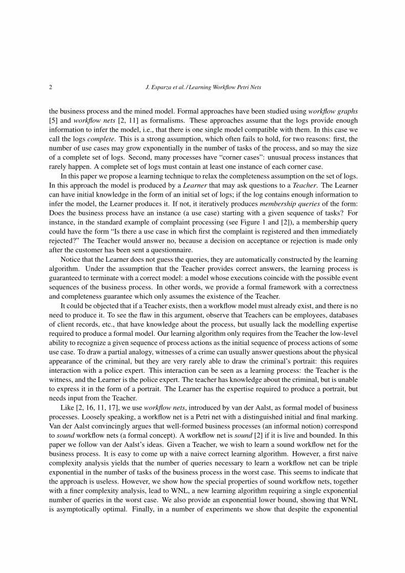
instance, in the standard example of complaint processing (see Figure 1 and [2]), a membership query
could have the form “Is there a use case in which first the complaint is registered and then immediately
rejected?” The Teacher would answer no, because a decision on acceptance or rejection is made only
after the customer has been sent a questionnaire.
Notice that the Learner does not guess the queries, they are automatically constructed by the learning
algorithm. Under the assumption that the Teacher provides correct answers, the learning process is
guaranteed to terminate with a correct model: a model whose executions coincide with the possible event
sequences of the business process. In other words, we provide a formal framework with a correctness
and completeness guarantee which only assumes the existence of the Teacher.
It could be objected that if a Teacher exists, then a workflow model must already exist, and there is no
need to produce it. To see the flaw in this argument, observe that Teachers can be employees, databases
of client records, etc., that have knowledge about the process, but usually lack the modelling expertise
required to produce a formal model. Our learning algorithm only requires from the Teacher the low-level
ability to recognize a given sequence of process actions as the initial sequence of process actions of some
use case. To draw a partial analogy, witnesses of a crime can usually answer questions about the physical
appearance of the criminal, but they are very rarely able to draw the criminal’s portrait: this requires
interaction with a police expert. This interaction can be seen as a learning process: the Teacher is the
witness, and the Learner is the police expert. The teacher has knowledge about the criminal, but is unable
to express it in the form of a portrait. The Learner has the expertise required to produce a portrait, but
needs input from the Teacher.
Like [2, 16, 11, 17], we use workflow nets, introduced by van der Aalst, as formal model of business
processes. Loosely speaking, a workflow net is a Petri net with a distinguished initial and final marking.
Van der Aalst convincingly argues that well-formed business processes (an informal notion) correspond
to sound workflow nets (a formal concept). A workflow net is sound [2] if it is live and bounded. In this
paper we follow van der Aalst’s ideas. Given a Teacher, we wish to learn a sound workflow net for the
business process. It is easy to come up with a naive correct learning algorithm. However, a first naive
complexity analysis yields that the number of queries necessary to learn a workflow net can be triple
exponential in the number of tasks of the business process in the worst case. This seems to indicate that
the approach is useless. However, we show how the special properties of sound workflow nets, together
with a finer complexity analysis, lead to WNL, a new learning algorithm requiring a single exponential
number of queries in the worst case. We also provide an exponential lower bound, showing that WNL
is asymptotically optimal. Finally, in a number of experiments we show that despite the exponential
J. Esparza et al. / Learning Workflow Petri Nets 3
worst-case complexity the algorithm is able to synthesize interesting workflows. Notice also that the
complexity is analysed for the case in which no initial event log is provided, that is, the case in which all
knowledge has to be extracted from the Teacher by asking membership queries.
Technically, the triple exponential complexity of the naive algorithm is a consequence of the follow-
ing three facts:
(a) the size of a deterministic finite automaton (DFA) recognizing the language of a net with n transi-
tions can be a priori double exponential in n;
(b) learning such a DFA using only membership queries requires exponentially many queries in the
size of the DFA (follows from [7] and [19, 15]); and
(c) the algorithms of Darondeau et al. for synthesis of Petri nets from regular languages [8] are expo-
nential in the size of the DFA.
In the paper we solve (a) by proving that the size of the DFA is only single exponential; we solve (b)
by exhibiting a better learning algorithm for sound workflow nets requiring only polynomially many
queries; finally, we solve (c) by showing that for sound workflow nets the algorithms for synthesis of
Petri nets from regular languages can be replaced by the algorithms for synthesis of bounded nets from
minimal DFA, which are of polynomial complexity. Notice that our solution very much profits from the
restriction to sound workflow nets, but that this restriction is given by the application domain: that sound
workflow nets are an adequate formalization of well-formed business processes has been proved by the
large success of the model in both the workflow modelling and Petri net communities.
Outline In the next section, we fix the notation of automata, recall the notion of Petri nets and workflow
nets, and cite results on synthesis of Petri nets from automata. Our learning algorithm WNL is elaborated
in Section 3. In Section 4 we describe some optimizations and heuristics to improve the performance of
our basic algorithm. Section 5 reports on our implementation and experimental results. Finally, we sum
up our contribution in the conclusion.
2. Preliminaries
We assume that the reader is familiar with elementary notions of graphs, automata and net theory. In this
section we fix some notations and define some less common notions.
2.1. Automata and Languages
A deterministic finite automaton (DFA) is a 5-tuple A = (Q,Σ, δ, q0, F ) where Q is a finite set of states,
Σ is a finite alphabet, q0 ∈ Q is the initial state, δ : Q × Σ → Q is the (partial) transition function and
F ⊆ Q is the set of final states. We denote by δ the function δ : Q × Σ∗ → Q inductively defined by
δ(q, ǫ) = q and δ(q, wa) = δ(δ(q, w), a). The language L(q) of some state q ∈ Q is the set of words
w ∈ Σ∗ such that δ(q, w) ∈ F . The language recognized by a DFA A is defined as L(A) := L(q0). A
language is regular if it is accepted by some DFA.
4 J. Esparza et al. / Learning Workflow Petri Nets
Myhill-Nerode theorem and minimal DFAs Given a language L ⊆ Σ∗, we say two words w,w′ ∈ Σ∗
are L-equivalent, denoted by w ∼L w′, if wv ∈ L ⇔ w′v ∈ L for every v ∈ Σ∗. The language L is
regular iff L-equivalence partitions Σ∗ into a finite number of equivalence classes. Given a regular
language L, there exists a unique DFA A up to isomorphism with a minimal number of states such that
L(A) = L; this automaton A is called the minimal DFA for L. The number of states of this automaton is
equal to the number of equivalence classes.
Given a DFA A = (Q,Σ, δ, q0, F ), we say two states q, q′ ∈ Q are A-equivalent if L(q) = L(q′).We can quotient A with respect to this equivalence relation. The states of the quotient DFA are the equiv-
alence classes of ∼A. The transitions are defined by “lifting” the transitions of A: for every transition
qa−→ q′, add [q]
a−→ [q′] to the transitions of the quotient DFA, where [q] and [q′] denote the equivalence
classes of q and q′. The initial state is [q0], and the final states are [q] | q ∈ F. The quotient DFA
recognizes the same language as A, and is isomorphic to the minimal DFA recognizing L.
It is easy to see that the minimal automaton for a prefix-closed regular language has a unique non-
final state (a trap state). For simplicity, we sometimes identify this automaton with the one obtained by
removing the trap state together with its ingoing and outgoing transitions.
2.2. Petri Nets
A (marked) Petri net is a 5-tuple N = (P, T, F,W,m0) where P is a set of places, T is a set of transitions
with P ∩ T = ∅, F ⊆ (P × T ) ∪ (T × P ) is a flow relation, W : (P × T ) ∪ (T × P )→ N is a weight
function satisfying W (x, y) > 0 iff (x, y) ∈ F , and m0 : P → N is a mapping called the initial marking.
For each transition or place x we call the set •x := y ∈ P ∪ T : (y, x) ∈ F the preset of x.
Analogously we call x• := y ∈ P ∪ T : (x, y) ∈ F the postset of x. A net is pure if no transition
belongs to both the pre- and postsets of some place.
Given an arbitrary but fixed numbering of P and T , the incidence matrix of N is the |P |×|T |-matrix
C given by: C(pi, tj) = W (tj , pi)−W (pi, tj).
A transition t ∈ T is enabled at a marking m, if ∀p ∈ •t : m(p) ≥ W (p, t). If a transition t is
enabled it can fire to produce the new marking m′, written as mt−→ m′.
m′(p) := m(p) +∑
p′∈P
C(p′, t)
Given w = t1 · · · tn ∈ T ∗ (i.e. ti ∈ T ), we write m0w−→ m if W = ε and m = m0 or there
exist markings m1, . . . ,mn such that mn = m and m0t1−→ m1
t2−→ m2 . . .mn−1tn−→ mn. Then,
we say that m is reachable. The set of reachable markings of N is denoted byM(N) and defined by
M(N) = m : ∃w ∈ T ∗. m0w−→ m. It is well-known that if m0
w−→ m, then m = m0 + C · P (w),
where P (w), the Parikh vector of w, is the vector of dimension |T | having as i-th component the number
of times that ti occurs in w. We call this equality the marking equation.
A net N is k-bounded if m(p) ≤ k for every reachable marking m and every place p of N , and
bounded if it is k-bounded for some k ≥ 0. A 1-bounded net is also called safe. A net is reversible if for
every firing sequence m0w−→ m there is a sequence vw leading back to the initial state, i.e. m
vw−→ m0.
N is live if every transition can fire eventually at every marking, i.e. ∀m ∈ M(N)∃wm.mwmt−→ m′ for
some m′.
J. Esparza et al. / Learning Workflow Petri Nets 5
i o
register
contact customer
contact department
collect
accept
reject
pay refund
send rejection
archive
need more info
acquire info
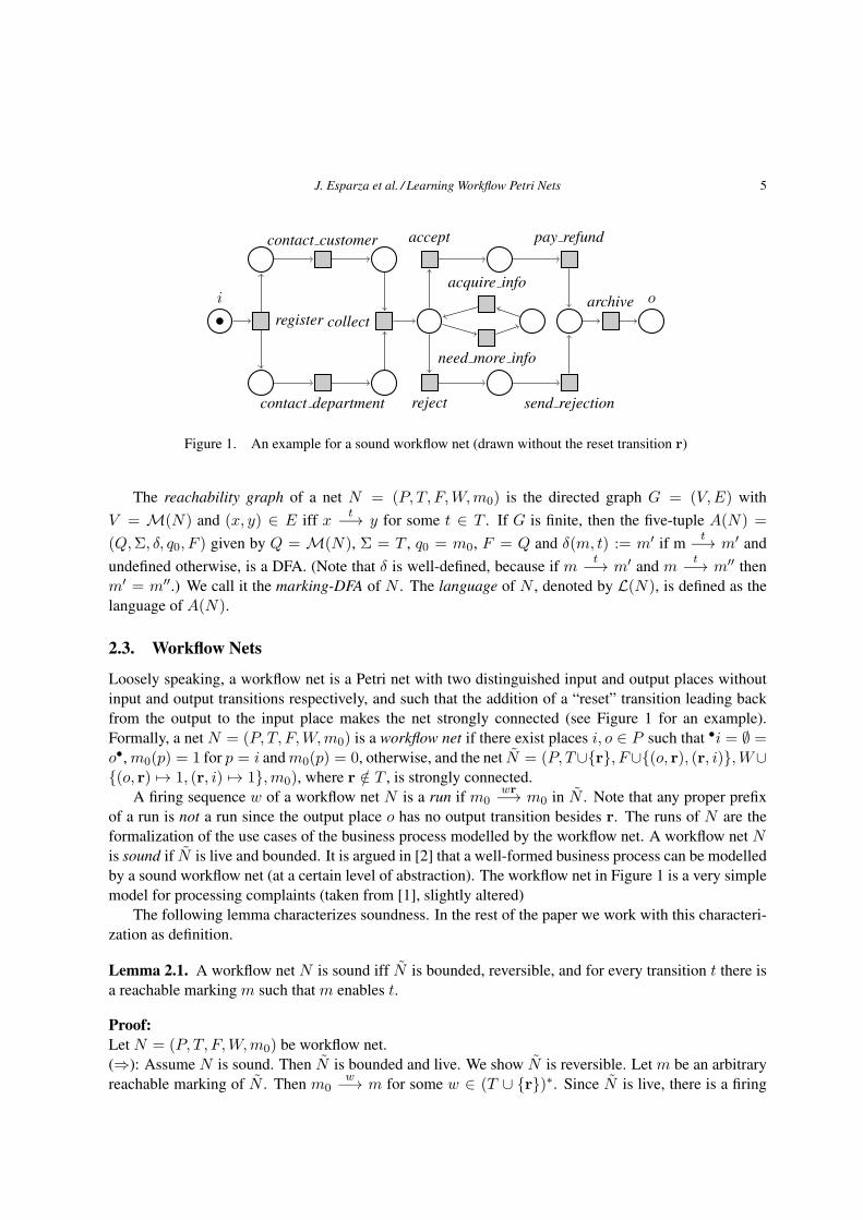
Figure 1. An example for a sound workflow net (drawn without the reset transition r)
The reachability graph of a net N = (P, T, F,W,m0) is the directed graph G = (V,E) with
V = M(N) and (x, y) ∈ E iff xt−→ y for some t ∈ T . If G is finite, then the five-tuple A(N) =
(Q,Σ, δ, q0, F ) given by Q =M(N), Σ = T , q0 = m0, F = Q and δ(m, t) := m′ if mt−→ m′ and
undefined otherwise, is a DFA. (Note that δ is well-defined, because if mt−→ m′ and m
t−→ m′′ then
m′ = m′′.) We call it the marking-DFA of N . The language of N , denoted by L(N), is defined as the
language of A(N).
2.3. Workflow Nets
Loosely speaking, a workflow net is a Petri net with two distinguished input and output places without
input and output transitions respectively, and such that the addition of a “reset” transition leading back
from the output to the input place makes the net strongly connected (see Figure 1 for an example).
Formally, a net N = (P, T, F,W,m0) is a workflow net if there exist places i, o ∈ P such that •i = ∅ =o•, m0(p) = 1 for p = i and m0(p) = 0, otherwise, and the net N = (P, T∪r, F∪(o, r), (r, i),W∪(o, r) 7→ 1, (r, i) 7→ 1,m0), where r /∈ T , is strongly connected.
A firing sequence w of a workflow net N is a run if m0wr
−→ m0 in N . Note that any proper prefix
of a run is not a run since the output place o has no output transition besides r. The runs of N are the
formalization of the use cases of the business process modelled by the workflow net. A workflow net Nis sound if N is live and bounded. It is argued in [2] that a well-formed business process can be modelled
by a sound workflow net (at a certain level of abstraction). The workflow net in Figure 1 is a very simple
model for processing complaints (taken from [1], slightly altered)
The following lemma characterizes soundness. In the rest of the paper we work with this characteri-
zation as definition.
Lemma 2.1. A workflow net N is sound iff N is bounded, reversible, and for every transition t there is
a reachable marking m such that m enables t.
Proof:
Let N = (P, T, F,W,m0) be workflow net.
(⇒): Assume N is sound. Then N is bounded and live. We show N is reversible. Let m be an arbitrary
reachable marking of N . Then m0w−→ m for some w ∈ (T ∪ r)∗. Since N is live, there is a firing
6 J. Esparza et al. / Learning Workflow Petri Nets
sequence w such that mwr
−→ m′ for some marking m′. We claim m′ = m0. Assume m′ 6= m0. Then,
since m′(i) > 0, we have m′(p) ≥ m0(p) for every place p, and m′(p) > m0(p) for some p. So m′
strictly covers m0, and so N is not bounded.
(⇐): Assume N is bounded, reversible and every transition is enabled at some reachable marking.
We show that N is live, which implies that N is sound. Let m be an arbitrary reachable marking of N ,
and let t ∈ T ∪ r. Since N is reversible, mw−→ m0 for some w ∈ (T ∪ r)∗, and since t occurs in
some firing sequence m0vt−→ m′ for some v ∈ (T ∪ r)∗ and some m′. So N is live (and bounded by
assumption) and therefore N is sound. ⊓⊔
2.4. Synthesis of Petri Nets from Languages and from Automata
In [8], Darondeau et al. address two synthesis problems of Petri nets from a minimal DFA A over an
alphabet T :
(S1) Decide if there is a bounded net N with T as set of transitions such that L(N) = L(A), and if so
return one. We call this problem synthesis up to language equivalence.
(S2) Decide if there is a bounded net N with T as set of transitions such that the reachability graph of
N is isomorphic to A, and if so return one. We call this problem synthesis up to isomorphism.
The algorithm of [8] for synthesis up to language equivalence works in two phases. Firstly, A is
transformed into an equivalent automaton A′ in a certain normal form. In the worst case, A′ can be
exponentially larger than A. The second phase constructs the net N , if it exists, in polynomial time in A′.
The algorithm requires exponential time in A. The algorithm of [8] for synthesis up to isomorphism, on
the contrary, needs only polynomial time in A. Notice that, in general, if one knows the language L(N)of a net, one does not know directly its marking-DFA. In particular, the minimal automaton recognizing
L(N) may not be the marking-DFA of any net. The basic algorithm in [8] can only handle pure nets, but
a generalization to non-pure nets can be found in [9].
Hints on how to obtain nets that are more “visually appealing” (i.e. have few arcs, no redundant
places, etc.) than those generated by standard synthesis algorithms can be found in [10], where net
synthesis was applied to process mining from event logs.
3. A Learning Algorithm for Sound Workflow Nets
Our goal is to develop a learning algorithm for sound workflow nets which is guaranteed to terminate,
and in which a teacher only needs to answer membership queries.
The precise learning setting is as follows. We have a Leaner and a Teacher. The Learner is given
a set T of transitions, where each transition corresponds to a dedicated task (in the sense of [2]) of the
business process. The Learner repeatedly asks the Teacher workflow membership queries. A query is a
sequence σ ∈ T ∗, and is answered by the Teacher as follows: if σ can be extended to a use case (i.e.,
a sequence corresponding to a complete instance of the business process), then the Teacher returns this
use case in the form of a transition sequence στr, where τ ∈ T ∗ (actually, we assume that the Teacher
just returns στ , the reset transition is implicitly always there). Otherwise, the Teacher answers “no”. In
our running example the Learner is given the set of transitions of the net of Figure 1, and the Teacher’s
answers are compatible with this net, i.e., acts as if it knew the net. Note that in practice, this only means
J. Esparza et al. / Learning Workflow Petri Nets 7
that the Teacher can either extend the query to a use case of the net to learn or can reject the query. Two
possible queries are
register contact customer contact department
register contact customer collect
A possible answer to the first query is the run
register contact customer contact department collect accept pay refund archive
while the answer to the second query is “no”.
Assuming that the Teacher’s answers are compatible with a k-bounded and reversible net N , the
goal of the Learner is to produce a net N ′ such that L(N) = L(N ′). It is easy to see that a (very
inefficient) learning algorithm exists for a given k known in advance. Since N is k-bounded, we need
only consider nets N ′ with arc weights smaller than or equal to k, and where no two places p, p′ satisfy
W (p, t) = W (p′, t) and W (t, p) = W (t, p′) for every transition t. (We can always remove one of p and
p′ without changing the language of the net.). Under these constraints we have:
(1) A net with n transitions has at most c1 := 2(2k+2)n places. (For each transition t we have k + 1possible values for each of W (p, t) and W (t, p).)
(2) By (1), N has at most c2 := (k+1)c1 reachable markings. Therefore, there exists a minimal DFA
A with at most c2 states such that L(N) = L(A).
(3) The minimal DFA A can be learned by querying all words over T of length 2c2, i.e., after at most
c3 := n2c2 queries.
To see this, observe first that any two prefix-closed minimal DFAs with c2 states differ in some
word of length c2. We now apply the Myhill-Nerode Theorem to construct A from the answers to
the queries as follows. The states of A are the equivalence classes of words of L(N) of length up
to c2, where two words w, v are equivalent if for every word u of length up to c2 either wu and
vu belong to L(N), or none of them does [19, 15]. The initial state is the equivalence class of the
empty word, and all states are final. There is a transition [w]a−→ [wa] for every word w of length
at most c2.
(4) The net N is obtained from A by means of the algorithm of [8] for synthesis up to language
equivalence (see problem (S1) in Section 2.4). The algorithm runs in 2O(p(c2)) time for some
polynomial p.
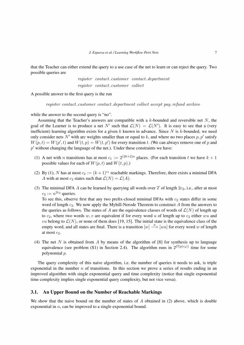
The query complexity of this naive algorithm, i.e. the number of queries it needs to ask, is triple
exponential in the number n of transitions. In this section we prove a series of results ending in an
improved algorithm with single exponential query and time complexity (notice that single exponential
time complexity implies single exponential query complexity, but not vice versa).
3.1. An Upper Bound on the Number of Reachable Markings
We show that the naive bound on the number of states of A obtained in (2) above, which is double
exponential in n, can be improved to a single exponential bound.
8 J. Esparza et al. / Learning Workflow Petri Nets
Given a net N = (P, T, F,W,m0) with incidence matrix C, we let C(p) denote the p-th row vector
(C(p, t1), . . . , C(p, t|T |)). We say that a place p is a linear combination of the places p1, . . . , pk if there
are real numbers λ1, . . . , λk such that C(p) =∑k
i=1 λi · C(pi).The following lemma is well known.
Lemma 3.1. Let N = (P, T, F,W,m0) be a net with incidence matrix C, and let C(p) =∑k
i=1 λiC(pi).
Then for every reachable marking m: ∀p ∈ P. m(p) = m0(p) +∑k
i=1 λi(m(pi)−m0(pi)) .
Proof:
Since m is reachable, there is w ∈ T ∗ such that m0w−→ m. By the marking equation m = m0+C ·P (w),
and so in particular m(p) = m0(p) + C(p) · P (w), and m(pi) = m0(pi) + C(pi) · P (w) for every
1 ≤ i ≤ k. So m(p) = m0(p) +∑k
i=1 λiC(pi) · P (w) = m0(p) +∑k
i=1 λi(m(pi)−m0(pi)) ⊓⊔
Theorem 3.1. Let N = (P, T, F,W,m0) be a k-bounded net with n transitions. Then N has at most
(k + 1)n reachable markings.
Proof:
The incidence matrix C has |P | rows and n columns, and so it has rank at most n. So there are l places
p1, . . . , pl, l ≤ n, such that C(p1), . . . , C(pl) are linearly independent. So every place p is a linear
combination of p1, . . . , pl. It follows from Lemma 3.1 that for every two reachable markings m,m′, if
m(pi) = m′(pi) for every 1 ≤ i ≤ l, then m(p) = m′(p) for every place p. In other words, if two
markings coincide on all of p1, . . . , pl, they are equal. Since for every reachable marking m we have
0 ≤ m(pi) ≤ k, the number of projections of the reachable markings onto the places p1, . . . , pl is at
most (k + 1)l ≤ (k + 1)n. So N has at most (k + 1)n reachable markings. ⊓⊔
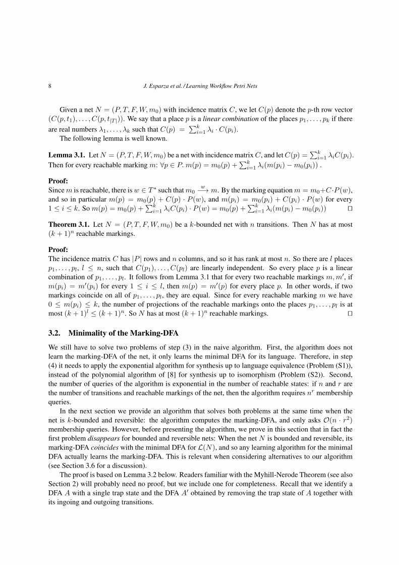
3.2. Minimality of the Marking-DFA
We still have to solve two problems of step (3) in the naive algorithm. First, the algorithm does not
learn the marking-DFA of the net, it only learns the minimal DFA for its language. Therefore, in step
(4) it needs to apply the exponential algorithm for synthesis up to language equivalence (Problem (S1)),
instead of the polynomial algorithm of [8] for synthesis up to isomorphism (Problem (S2)). Second,
the number of queries of the algorithm is exponential in the number of reachable states: if n and r are
the number of transitions and reachable markings of the net, then the algorithm requires nr membership
queries.
In the next section we provide an algorithm that solves both problems at the same time when the
net is k-bounded and reversible: the algorithm computes the marking-DFA, and only asks O(n · r2)membership queries. However, before presenting the algorithm, we prove in this section that in fact the
first problem disappears for bounded and reversible nets: When the net N is bounded and reversible, its
marking-DFA coincides with the minimal DFA for L(N), and so any learning algorithm for the minimal
DFA actually learns the marking-DFA. This is relevant when considering alternatives to our algorithm
(see Section 3.6 for a discussion).
The proof is based on Lemma 3.2 below. Readers familiar with the Myhill-Nerode Theorem (see also
Section 2) will probably need no proof, but we include one for completeness. Recall that we identify a
DFA A with a single trap state and the DFA A′ obtained by removing the trap state of A together with
its ingoing and outgoing transitions.
J. Esparza et al. / Learning Workflow Petri Nets 9
Lemma 3.2. A DFA A = (Q,Σ, δ, q0, F ) is minimal iff the following two conditions hold:
(1) every state lies in a path leading from q0 to some state of F , and
(2) L(q) 6= L(q′) for every two distinct states q, q′ ∈ Q.
Proof:
(⇒): We prove the contrapositive. For (1), if some state q does not lie in any path from q0 to some
final state, then it can be removed without changing the language, and so A is not minimal. For (2), if
two distinct states q, q′ of A satisfy L(q) = L(q′), then [q] = [q′], and so the quotient automaton has
fewer states than A. So A is not minimal.
(⇐): Assume (1) and (2) hold. We prove that for every state q the language of the words w such that
δ(q0, w) = q is an equivalence class of L-equivalence. It follows that the number of states of A is at
most as large as the number of equivalence classes of L-equivalence, which implies that A is the minimal
DFA for L.
It suffices to show:
• If δ(q0, w) = q = δ(q0, v), then w ∼L v.
This follows immediately from the definition of L-equivalence.
• If δ(q0, w) = q and δ(q0, v) = q′ for some q′ 6= q, then w 6∼L v.
Since L(q) 6= L(q′), w.l.o.g. there is a word u ∈ L(q) \ L(q′). So wu ∈ L and vu /∈ L, which
implies w 6∼L v.
⊓⊔
Theorem 3.2. Let N = (P, T, F,W,m0) be a bounded and reversible Petri net. The marking-DFA
A(N) of N is a minimal DFA.
Proof:
Since N is bounded, A(N) is a DFA. Assume that A(N) is not minimal. Since every state of A(N)is final, by Lemma 3.2 there are two states of A(N), i.e., two reachable markings m1 6= m2 of N ,
such that L(m1) = L(m2). As m1 6= m2 there exists p ∈ P with m1(p) 6= m2(p). Assume w.l.o.g.
m1(p) < m2(p). Let m be a reachable marking such that m(p) is minimal, i.e. there is no other
reachable marking m′ s.t. m′(p) < m(p). Since m is reachable and N is reversible, there is w ∈ T ∗
such that m2w−→ m. Since L(m1) = L(m2), there is a reachable marking m′ such that m1
w−→ m′. It
follows
m′(p) = m1(p) + C(p) · P (w) < m2(p) + C(p) · P (w) = m(p)
contradicting the minimality of m(p). ⊓⊔
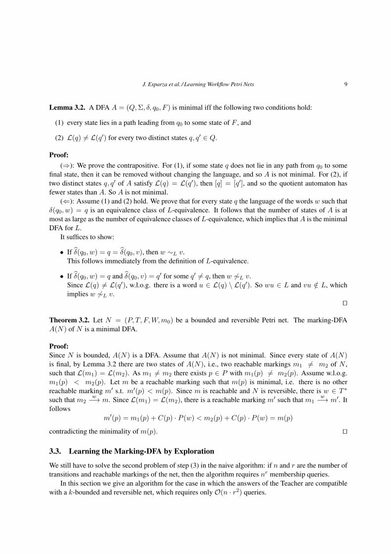
3.3. Learning the Marking-DFA by Exploration
We still have to solve the second problem of step (3) in the naive algorithm: if n and r are the number of
transitions and reachable markings of the net, then the algorithm requires nr membership queries.
In this section we give an algorithm for the case in which the answers of the Teacher are compatible
with a k-bounded and reversible net, which requires only O(n · r2) queries.
10 J. Esparza et al. / Learning Workflow Petri Nets
Recall the standard search approach for constructing the reachability graph of a net if the net is known.
We maintain a queue of markings, initially containing the initial marking, and two sets of already visited
markings and transitions (transitions between markings). While the queue is non-empty, we take the
marking m at the top of the queue, and check for each transition a whether a is enabled at m. If so, we
compute the marking m′ such that ma−→ m′, and proceed as follows: if m′ has been already visited,
we add ma−→ m′ to the set of visited transitions; if m′ had not been visited yet, we add m′ to the set of
visited markings and to the queue, and add ma−→ m′ to the set of visited transitions.
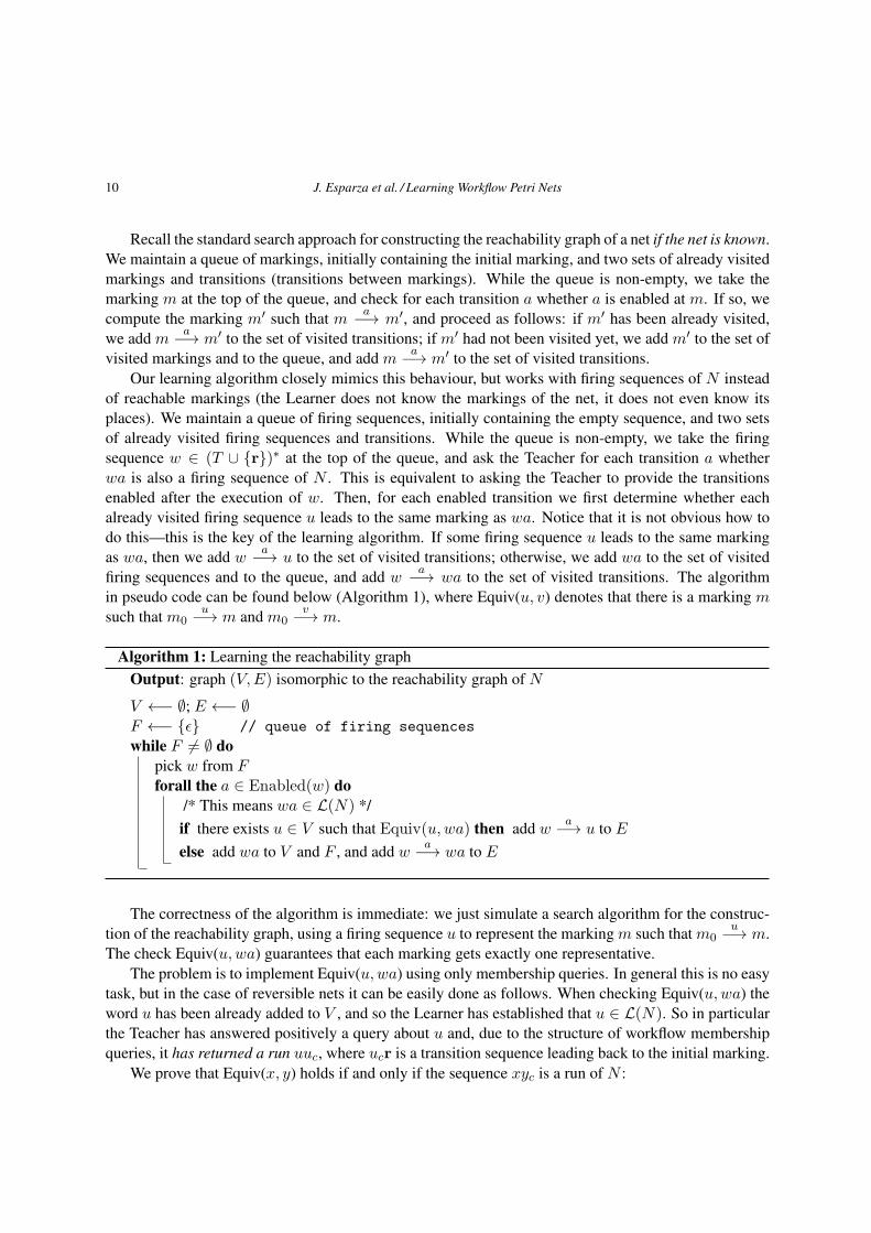
Our learning algorithm closely mimics this behaviour, but works with firing sequences of N instead
of reachable markings (the Learner does not know the markings of the net, it does not even know its
places). We maintain a queue of firing sequences, initially containing the empty sequence, and two sets
of already visited firing sequences and transitions. While the queue is non-empty, we take the firing
sequence w ∈ (T ∪ r)∗ at the top of the queue, and ask the Teacher for each transition a whether
wa is also a firing sequence of N . This is equivalent to asking the Teacher to provide the transitions
enabled after the execution of w. Then, for each enabled transition we first determine whether each
already visited firing sequence u leads to the same marking as wa. Notice that it is not obvious how to
do this—this is the key of the learning algorithm. If some firing sequence u leads to the same marking
as wa, then we add wa−→ u to the set of visited transitions; otherwise, we add wa to the set of visited
firing sequences and to the queue, and add wa−→ wa to the set of visited transitions. The algorithm
in pseudo code can be found below (Algorithm 1), where Equiv(u, v) denotes that there is a marking msuch that m0
u−→ m and m0
v−→ m.
Algorithm 1: Learning the reachability graph
Output: graph (V,E) isomorphic to the reachability graph of N
V ←− ∅; E ←− ∅F ←− ǫ // queue of firing sequences
while F 6= ∅ do
pick w from Fforall the a ∈ Enabled(w) do
/* This means wa ∈ L(N) */
if there exists u ∈ V such that Equiv(u,wa) then add wa−→ u to E
else add wa to V and F , and add wa−→ wa to E
The correctness of the algorithm is immediate: we just simulate a search algorithm for the construc-
tion of the reachability graph, using a firing sequence u to represent the marking m such that m0u−→ m.
The check Equiv(u,wa) guarantees that each marking gets exactly one representative.
The problem is to implement Equiv(u,wa) using only membership queries. In general this is no easy
task, but in the case of reversible nets it can be easily done as follows. When checking Equiv(u,wa) the
word u has been already added to V , and so the Learner has established that u ∈ L(N). So in particular
the Teacher has answered positively a query about u and, due to the structure of workflow membership
queries, it has returned a run uuc, where ucr is a transition sequence leading back to the initial marking.
We prove that Equiv(x, y) holds if and only if the sequence xyc is a run of N :
J. Esparza et al. / Learning Workflow Petri Nets 11
Proposition 3.1. In Algorithm 1, Equiv(u,wa) = true if and only if uwc is a run of N , where wawc is
the run reported by the Teacher when positively answering the query about wa ∈ L(N).
Proof:
If Equiv(u,wa) = true, then there is a marking m such that m0u−→ m and m0
wa−→ m. Because
m0wa−→ m
wcr−→ m0, we have m0u−→ m
wcr−→ m0, which implies that uwc is a run.
If u · wc is a run, then we have m0wawcr−→ m0 and m0
uwcr−→ m0. Let m be the marking such that
m0wa−→ m. We then have m
wcr−→ m0. Moreover, m is the only marking such that mwcr−→ m0 (Petri
nets are backward deterministic: given a firing sequence and its target marking, the source marking is
uniquely determined). Since m0uwcr−→ m0, we then necessarily have m0
u−→ m
wcr−→ m0, and so in
particular m0u−→ m. So both wa and u lead to the same marking m, and we have Equiv(u,wa) =
true. ⊓⊔
We can now easily show that checking Equiv(u,wa) reduces to one single membership query.
Proposition 3.2. The check Equiv(u,wa) can be performed by querying whether uwc belongs to L(N):Equiv(u,wa) holds if and only if the Teacher answers positively and returns the sequence uwc itself as a
run.
Proof:
There are three possible cases:
• The answer is negative. Then uwc /∈ L(N), and so in particular it is not a run of N . So
Equiv(u,wa) = false.
• The answer is positive and the Teacher returns uwc as run. Then Equiv(u,wa) = true by Proposi-
tion 3.1.
• The answer is positive, but the Teacher returns uwcv for some v 6= ǫ as a run. Since no proper
prefix uwcv′ is a run (see the definition of a run in section 2.3), we have in particular by taking
v′ = ǫ that uwc is not a run. By Proposition 3.1 we have Equiv(u,wa) = false.⊓⊔
There is a technical issue that should be mentioned at this point. The algorithm delivers a net N ′ such
that the reachability graphs of N and N ′ are isomorphic. It follows that N ′ is reversible and bounded.
However, we cannot guarantee that N ′ has the same bound as N . For a trivial example, consider a net
consisting of a single circuit in which all arcs have weight k ≥ 1, with an initial marking that puts ktokens in a place and no tokens in the rest. Obviously, the reachability graph does not depend on k up
to isomorphism. We consider this fact a minor problem, since N ′ and N are equivalent for behavioural
purposes.
3.3.1. Complexity
It would seem natural to define the complexity of the algorithm as the total number of queries made
to the Teacher. (Since, as we have just shown, an equivalence query reduces to a membership query,
there is no need to distinguish between membership and equivalence queries). However, a finer analysis
12 J. Esparza et al. / Learning Workflow Petri Nets
shows that this measure is not adequate. In order to compute the set Enabled(w), the algorithm asks the
Teacher for every transition a whether wa is a firing sequence. This would count as |T | membership
queries. However, in a real-world workflow, even of moderate size, the number of transitions enabled at
a marking is much smaller than the total number of transitions, and so most of the queries are answered
negatively. As an extreme case, consider the task of learning the sequence of calendar months. The
algorithm starts with the empty sequence, and then ask twelve membership queries of the form “Can
January, February, . . . , December ?” . Obviously, any human Teacher would prefer to be asked “Which
is the first month of the year?” (or “Which could be the first months of the year?” if the Learner does not
know that months are totally ordered).
This would suggest to count a call to Enabled() as one single query. However, this is also misleading:
because of the way equivalence queries are dealt with, the Teacher must provide for every positively
answered query an extension of the query sequence to a run. For this reason, it is more adequate to use
the following complexity measure: if a call to Enabled() returns k enabled transitions, then we assign
to it a cost of k membership queries, but each call to Equiv() counts as one membership query. (Notice
that the membership query for an equivalence query asks if uwc is fireable, where only u is known to be
fireable.)
Let r be the number of reachable markings of N , and let d be the enabling degree of N , i.e., the
maximum number of transitions of N that can be enabled by a reachable marking. It follows from the
description of Algorithm 1 that the number of firing sequences added to the queue is equal to r. Now,
let w be the i-th sequence taken from the queue (i.e., w is taken from the queue when |V | = i − 1).
Processing w requires at most d · i membership queries: d queries for the call to Enabled(), and at most
d · (i − 1) equivalence checks of the form Equiv(u,wa) (because u ∈ V and a ∈ E). So the algorithm
performs at most∑r
i=1 d · i = dr(r + 1)/2 ∈ O(d · r2) queries.
Putting all the pieces of our discussion together, we obtain WNL, an algorithm to learn a bounded
and reversible net N . WNL proceeds as follows:
• Using Algorithm 1, learn the marking-DFA A of N .
• Apply the polynomial algorithm of [8] for synthesis up to isomorphism (S2).
The following theorem sums up the results of the section.
Theorem 3.3. (Learning by Exploration)
Let N be a k-bounded and reversible net N with n transitions and enabling degree d. WNL returns a
bounded net N ′ such that L(N) = L(N ′). Moreover, WNL requires at most O(d · (k + 1)2n) queries,
and the total runtime of the Learner is polynomial in k and d, and single exponential in n.
Proof:
The correctness follows immediately from the fact that Algorithm 1 returns the marking-DFA of N (up
to isomorphism).
For the bound on the number of queries, we observe that, by the discussion above, Algorithm 1 asks
O(d ·r2) queries, where r is the number of reachable states, and that r ≤ (k+1)n holds by Theorem 3.1.
For the exponential bound on the runtime, observe that Algorithm 1 explores firing sequences by
increasing length. Therefore, if a sequence w leading to a marking m is added to the queue, then w is
a shortest sequence leading to w. Since the net has at most (k + 1)n reachable markings, the length
of w is at most (k + 1)n. Therefore, the Learner needs O((k + 1)n) time to perform an operation on
J. Esparza et al. / Learning Workflow Petri Nets 13
a sequence. Since the number of operations is polynomial in the number of queries, the runtime is in
O(d · r2 · (k + 1)n), and thus polynomial in k and d, and single exponential in n. ⊓⊔
Notice that we only give a bound for the runtime of the Learner. The runtime of the Teacher depends
on the computational model associated to her. For the case in which the Teacher consults an event log
(i.e., a database of runs), see Section 3.4.
A final question is what happens if the Teacher’s answers are not compatible with any k-bounded and
reversible net N . In this case there are two possibilities: they are not compatible with any DFA having at
most (k+ 1)n states, or they are compatible with some such DFA, but this DFA is not the marking-DFA
of any net. In the first case the algorithm can stop when the number of generated states exceeds (k+1)n.
In the second case, the algorithm terminates and produces a DFA, but the synthesis algorithm of [8] does
not return a net.
3.4. Mixing Process Mining and Learning
The algorithm we have just presented does not assume the existence of an event log: the Learner only
gets information from membership queries. However, as explained in the introduction, we consider our
learning approach as a way of complementing log-based process mining. In this section we explain how
to modify the algorithm accordingly.
We assume the existence of an event log consisting of use cases. Given the set of tasks T of the
business process, we can think of each use case as a word w ∈ T ∗, such that w corresponds to a run of
the reversible net to be learnt. The event log then corresponds to a language L ⊆ T ∗.
In a first step we construct a minimal DFA for the language L. This can be done space-efficiently in
a number of ways. For instance, we can divide the set of runs in two halves L1, L2, recursively compute
minimal DFAs A1, A2 recognizing L1 and L2, and then compute the minimal DFA for L from A1, A2
using an algorithm very similar to the one that computes the union of two binary decision diagrams [6].
Once this is done, we easily get the minimal DFA A for the language of prefixes of (Lr)∗ (this requires
to add one extra state and make all states final).
Once A is computed, we assign to each state q of A a word wq such that q0wq−→ q. For every two
states q1, q2, we check whether the states correspond to the same reachable marking by calling Equiv(wq1 ,
wq2). After this step we are in the same situation we would have reached if the algorithm would have
queried all the words wq.
In practice we would first apply the reduction techniques described in Section 4 before actually
calling Equiv() for each pair of states, which would be quite inefficient.
3.5. A Lower Bound for Petri Net Learning
We now show that we cannot in general solve the learning problem in subexponential time, by providing
a hard-to-learn instance. We will show that any learning algorithm has to ask Ω(2n) membership queries
in the worst case to derive the correct net, where n is the number of transitions.
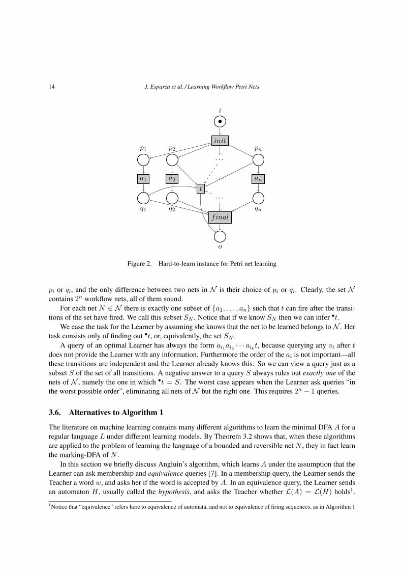
Consider the following set N of workflow nets. All the nets in N have the same number n + 3 of
transitions: two transitions init and final, transitions called a1, . . . , an, and a transition t (see Figure 2).
The pre- and postsets of all transitions but t, which are identical for all nets ofN , are shown in the figure.
The postset of t is always the place o. The preset of t always contains for each i exactly one of the places
14 J. Esparza et al. / Learning Workflow Petri Nets
p1 p2
· · ·
· · ·
pn
i
init
q1 q2
· · ·
qn
a1 a2 an
o
final
t
Figure 2. Hard-to-learn instance for Petri net learning
pi or qi, and the only difference between two nets in N is their choice of pi or qi. Clearly, the set Ncontains 2n workflow nets, all of them sound.
For each net N ∈ N there is exactly one subset of a1, . . . , an such that t can fire after the transi-
tions of the set have fired. We call this subset SN . Notice that if we know SN then we can infer •t.
We ease the task for the Learner by assuming she knows that the net to be learned belongs toN . Her
task consists only of finding out •t, or, equivalently, the set SN .
A query of an optimal Learner has always the form ai1ai2 · · · aikt, because querying any ai after tdoes not provide the Learner with any information. Furthermore the order of the ai is not important—all
these transitions are independent and the Learner already knows this. So we can view a query just as a
subset S of the set of all transitions. A negative answer to a query S always rules out exactly one of the
nets of N , namely the one in which •t = S. The worst case appears when the Learner ask queries “in
the worst possible order”, eliminating all nets of N but the right one. This requires 2n − 1 queries.
3.6. Alternatives to Algorithm 1
The literature on machine learning contains many different algorithms to learn the minimal DFA A for a
regular language L under different learning models. By Theorem 3.2 shows that, when these algorithms
are applied to the problem of learning the language of a bounded and reversible net N , they in fact learn
the marking-DFA of N .
In this section we briefly discuss Angluin’s algorithm, which learns A under the assumption that the
Learner can ask membership and equivalence queries [7]. In a membership query, the Learner sends the
Teacher a word w, and asks her if the word is accepted by A. In an equivalence query, the Learner sends
an automaton H , usually called the hypothesis, and asks the Teacher whether L(A) = L(H) holds1.
1Notice that “equivalence” refers here to equivalence of automata, and not to equivalence of firing sequences, as in Algorithm 1
J. Esparza et al. / Learning Workflow Petri Nets 15
If L(A) = L(H) the Teacher answers an equivalence query with “yes” or provides the Learner with a
counterexample w otherwise, i.e. w is a word in the symmetric difference of L(A) and L(H). If m is the
maximum length of a counterexample provided by the Teacher, Angluin’s algorithm learns a minimal
DFA with r states and alphabet size n using at mostO(n ·m · r2) membership queries and r equivalence
queries. Observe that the answer to a membership query is only “yes” or “no”, the Teacher is not required
to extend a firing sequence of the net to a run.
There is a trade-off between our learning setting and Angluin’s. Angluin’s setting requires an equiv-
alence oracle, but membership queries can be answered with a simple “yes/no”. On the other hand, our
setting does not need equivalence queries — at the price of requiring the Teacher to provide full runs.
Depending on the application (workflow design, requirements elicitation, reverse engineering of “black-
box” systems, etc.) both approaches can be useful, and Theorem 3.2 shows that both can be applied if
the workflow models are bounded and reversible.
4. Optimizations
In this section we discuss some simple heuristics and optimizations that can greatly reduce the number
of membership queries that the Teacher needs to answer.
There are some easy properties of Petri nets that can be used to reduce the number of queries in many
situations. Additionally, they are helpful to trim an initial DFA constructed from event logs.
4.1. Memorizing and Deducing Answers from a Partial DFA
A first obvious improvement on Algorithm 1 consists of storing the queries that have been already been
asked, together with the Teacher’s answer, and making sure that the Teacher is never asked the same
query twice. This also means not asking the Teacher to produce a run when one is already available.
Imagine that when asked Enabled(w) the Teacher answers that a is enabled by w, and wabc is a run.
If the algorithm asks now after Enabled(wa), it already knows that b belongs to it, and wabc is also a
witness run. So the Teacher is told not to provide this run.
A second easy optimization looks as follows. During its execution, Algorithm 1 learns that some
transition sequences are fireable, and others are not: more precisely, for each dequeued sequence wthe algorithm learns that wa is fireable for every a ∈ Enabled(w), and non-fireable for every a /∈Enabled(w). Moreover, the algorithm also learns that every prefix of a run returned by the Teacher
is fireable. An obvious optimization is to use this information to reduce the number of equivalence
queries passed to the Teacher. Recall that, when calling Equiv(u,wa), Algorithm 1 asks the Teacher
if uwc ∈ L(N), where wawc is the run reported by the Teacher when positively answering the query
about wa ∈ L(N) (see Proposition 3.2). Before asking the Teacher whether uwc ∈ L(N), the improved
algorithm first checks if it already knows whether uwc is a prefix of some fireable sequence, or whether
some prefix of uwc is not fireable. Our implementation (cf. Section 5) incorporates this improvement.
Notice that the equivalence query Equiv(u,wa) can also be answered by deciding if wauc ∈ L(N)holds, and is a run. However, in this case the algorithm would never be able to answer the query without
passing it to the Teacher, because wa is fireable, and the algorithm has not yet explored any sequence
having wa as a proper prefix.
16 J. Esparza et al. / Learning Workflow Petri Nets
4.2. Bounded Lookahead
In Algorithm 1, the answer to a query Equiv(u,wa) is positive iff the sequences u and wa are both
fireable, and lead to the same marking. So, in particular, if Equiv(u,wa) holds then for every transition
sequence v we have that uv is fireable iff wa is fireable. We can use this property to simplify the task
of the Teacher. Instead of directly asking whether Equiv(u,wa) holds, the algorithm asks the Teacher to
first provide the sets Enabled(u) and Enabled(wa). If the answers are different, then there is a transition
b such that exactly one of ub and wab is fireable, and so Equiv(u,wa) does not hold. (Note that the
Teacher does not have to provide full runs for any of these possible extensions so this is quite a simple
task.) We call this heuristic bounded lookahead of depth 1. The heuristic can be further extended by
asking the Teacher to provide the sequences of length d enabled by u and wa (lookahead of depth d). If
we explore possible extensions up to depth d we may ask up to |T |d unnecessary queries in case of an
already discovered state, but we can save up to n calls to Equiv(), if n is the number of states currently
discovered.
4.3. Parikh Vectors
It is well known that if w1, w2 ∈ L(N) and P (w1) = P (w2) (i.e., w1 and w2 have the same Parikh
vector) then firing w1 and w2 leads to the same marking. This fact can be used to reduce the number
of calls to Equiv() in our algorithm. For each state q in our currently explored automaton, we save the
Parikh vectors Pq of the words leading to it. Now, if the algorithm is currently processing w, and the
Teacher reported that w enables a transition a, then we check if P (wa) ∈ Pq for some state q. If that is
the case, then we simply add the transition pa−→ q.
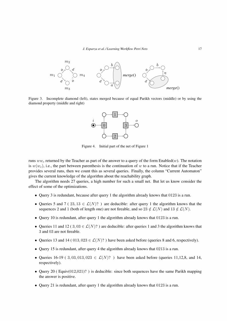
4.4. Diamond Property for Pure Nets
This heuristic saves queries when the net is required to be pure (i.e., when one can assume that if there is
a workflow net modelling the system, then there is also a pure workflow net). A diamond is a subgraph
in the reachability graph of a net with four states that are connected in the following way: m1a−→ m2,
m1b−→ m3, m2
b−→ m4, m3
a−→ m4. A diamond is incomplete if it is missing exactly one transition
(see Figure 3). It is well known that the reachability graphs of pure nets do not have incomplete diamonds
(the diamond property). Therefore, if the algorithm discovers that the part of the reachability graph
constructed so far has an incomplete diamond, it can directly add the missing transition, saving one
membership query and n equivalence queries, where n is the number of states constructed so far.
The diamond property can also be used to merge states of a DFA generated from an event log (see
Section 3.4 ) as indicated in Figure 3.
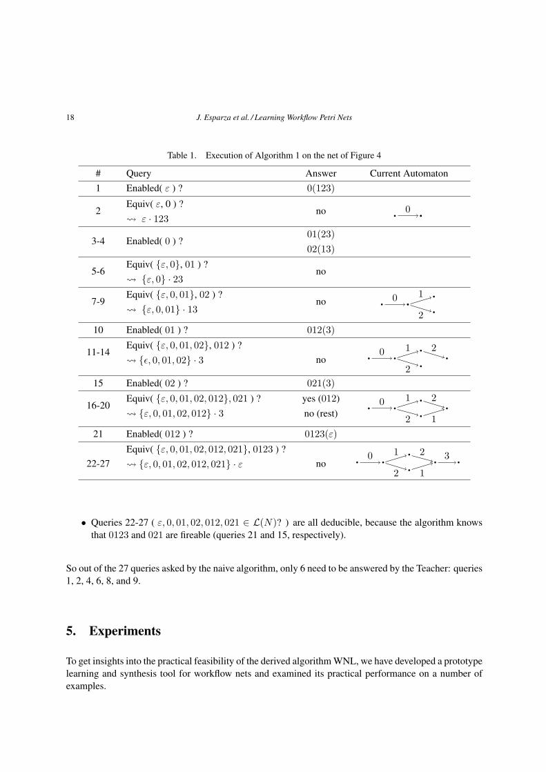
4.5. An Example
We show how Algorithm 1 learns the reachability graph of the net of Figure 4, the first part of the net
in Figure 1. Table 1 shows the list queries submitted to the Teacher when none of the optimizations
we have just discussed are applied. To simplify the presentation some queries are grouped together.
The “Query” column contains the queries being asked; Equiv(w1, . . . , wn, w) is an abbreviation for
Equiv(w1, w), . . . , Equiv(wn, w). The notation w1, . . . , wn·v indicates that the equivalence queries
are transformed into the membership queries w1v, . . . wnv. The “Answer” column contains the run or
J. Esparza et al. / Learning Workflow Petri Nets 17
merge()
merge()
m1
m2
m3
m4
a
b
b
a
a
b
b
a
a
b
b
a
Figure 3. Incomplete diamond (left), states merged because of equal Parikh vectors (middle) or by using the
diamond property (middle and right)
i o0
1
2
3
Figure 4. Initial part of the net of Figure 1
runs wwc returned by the Teacher as part of the answer to a query of the form Enabled(w). The notation
is w(wc), i.e., the part between parenthesis is the continuation of w to a run. Notice that if the Teacher
provides several runs, then we count this as several queries. Finally, the column “Current Automaton”
gives the current knowledge of the algorithm about the reachability graph.
The algorithm needs 27 queries, a high number for such a small net. But let us know consider the
effect of some of the optimizations.
• Query 3 is redundant, because after query 1 the algorithm already knows that 0123 is a run.
• Queries 5 and 7 ( 23, 13 ∈ L(N)? ) are deducible: after query 1 the algorithm knows that the
sequences 2 and 1 (both of length one) are not fireable, and so 23 /∈ L(N) and 13 /∈ L(N).
• Query 10 is redundant, after query 1 the algorithm already knows that 0123 is a run.
• Queries 11 and 12 ( 3, 03 ∈ L(N)? ) are deducible: after queries 1 and 3 the algorithm knows that
3 and 03 are not fireable.
• Queries 13 and 14 ( 013, 023 ∈ L(N)? ) have been asked before (queries 8 and 6, respectively).
• Query 15 is redundant, after query 4 the algorithm already knows that 0213 is a run.
• Queries 16-19 ( 3, 03, 013, 023 ∈ L(N)? ) have been asked before (queries 11,12,8, and 14,
respectively).
• Query 20 ( Equiv(012,021)? ) is deducible: since both sequences have the same Parikh mapping
the answer is positive.
• Query 21 is redundant, after query 1 the algorithm already knows that 0123 is a run.
18 J. Esparza et al. / Learning Workflow Petri Nets
Table 1. Execution of Algorithm 1 on the net of Figure 4
# Query Answer Current Automaton
1 Enabled( ε ) ? 0(123)
2Equiv( ε, 0 ) ?
no 0 ε · 123
3-4 Enabled( 0 ) ?01(23)
02(13)
5-6Equiv( ε, 0, 01 ) ?
no ε, 0 · 23
7-9Equiv( ε, 0, 01, 02 ) ?
no 0 1
2 ε, 0, 01 · 13
10 Enabled( 01 ) ? 012(3)
11-14Equiv( ε, 0, 01, 02, 012 ) ?
no0 1
2
2 ǫ, 0, 01, 02 · 3
15 Enabled( 02 ) ? 021(3)
16-20Equiv( ε, 0, 01, 02, 012, 021 ) ? yes (012) 0 1
2
2
1 ε, 0, 01, 02, 012 · 3 no (rest)
21 Enabled( 012 ) ? 0123(ε)
22-27
Equiv( ε, 0, 01, 02, 012, 021, 0123 ) ?
no0 1
2
2
1
3 ε, 0, 01, 02, 012, 021 · ε
• Queries 22-27 ( ε, 0, 01, 02, 012, 021 ∈ L(N)? ) are all deducible, because the algorithm knows
that 0123 and 021 are fireable (queries 21 and 15, respectively).
So out of the 27 queries asked by the naive algorithm, only 6 need to be answered by the Teacher: queries
1, 2, 4, 6, 8, and 9.
5. Experiments
To get insights into the practical feasibility of the derived algorithm WNL, we have developed a prototype
learning and synthesis tool for workflow nets and examined its practical performance on a number of
examples.
J. Esparza et al. / Learning Workflow Petri Nets 19
5.1. Implementation
Our prototype, which we call WNL for Workflow Net Learner, is written in C++. It has approximately
3,000 lines of code and uses LIBALF for dealing with automata. LIBALF is part of the automata learning
factory currently developed jointly at RWTH Aachen and TU MALnchen2 [14].
The synthesis algorithm (S2) of [8] is implemented using the LP SOLVE3 framework to efficiently
solve the linear programs needed for computing the places of the net. Furthermore LP SOLVE is used
for eliminating redundant places after the net has been synthesized to reduce its size and to make it
look more appealing. The implementation is currently not tailored to user interaction but consults pre-
existing workflow nets for queries. Outputs are given in form of dot-files that can be visualized using the
GRAPHVIZ toolkit.
5.2. Experimental Results
We have tested the performance of WNL on several pure, safe and reversible net models. The list of
models can be found in Table 2. The buf_n net models a n-buffer with 2 reachable markings, and
is especially suitable to illustrate scalability issues of the algorithms. The mutex_n models a mutual
exclusion algorithm for n processes. The absence workflow is loosely modelled after an example from
[18], and the complaint workflow is the example presented in our background section (Figure 1). The
order_simp and transit1 models are case studies taken from [20].
We have conducted two series of experiments. First, we apply WNL without any event logs as initial
knowledge, and then again with randomly generated logs as input. In both cases we count the number of
queries needed to learn the model. Recall that, besides counting the queries needed for Equiv(), we only
count queries answered positively by the Teacher, as these correspond to runs supplied by him, and thus
reflect the actual work to be done by an expert in an adequate manner.
5.2.1. Learning from Scratch
Table 2 collects the performance of WNL when learning a model “from scratch” with respect to the
size of the alphabet and the reachability graph, see Figure 2. The first two columns of the table give
the alphabet size and the number of reachable states of the model. The third column gives the number
of queries asked by the “non-optimized” algorithm. This is the algorithm that memorizes and deduces
answers to queries (see Section 4.1), but uses none of the further optimizations (bounded lookahead,
diamond property, Parikh-vectors).
The series of the n-cell buffer examples from n = 2 to n = 8 suggests that the practical performance
of WNL is even better than quadratic in the number of reachable markings. The time needed for learning
the nets in an applied setting is of course dominated by the number of queries a user has to answer.
Synthesizing the resulting Petri net using the method proposed by Darondeau et al. (see Section 2.4)
together with some post-processing to remove redundant places needs just a few seconds in the worst
case and is therefore negligible.
2http://libalf.informatik.rwth-aachen.de/3http://lpsolve.sourceforge.net/
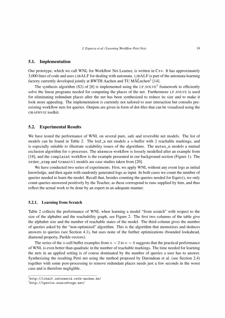
20 J. Esparza et al. / Learning Workflow Petri Nets
Table 2. Learning without logs: impact of optimizations on the number of queries. B=bounded lookahead of
depth 1, D=diamond heuristic, P = Parikh heuristic
Model |T | |RG| non-opt. +B +D +P +B+D +B+P +B+P+D
buf_2 3 4 6 12 5 6 10 12 10
buf_3 4 8 16 32 11 15 21 29 21
buf_4 5 16 50 85 31 43 46 69 46
buf_5 6 32 171 216 97 128 99 158 99
buf_6 7 64 599 538 312 390 216 359 216
buf_7 8 128 2115 1304 1013 1197 461 798 461
buf_8 9 256 7622 3107 3357 3778 994 1765 994
mutex_2 6 8 23 40 19 22 30 37 27
mutex_3 9 20 119 168 98 106 102 148 82
mutex_4 12 48 578 594 502 478 310 509 225
absence 11 8 21 32 21 21 32 32 32
complaint 12 11 26 37 24 25 34 35 34
order_simp 9 7 17 23 17 17 23 23 23
transit1 25 77 883 474 439 504 221 287 221
Impact of Optimizations. The rest of Table 2 describes the impact of the different optimizations and
combinations thereof on the total number of queries. Observe that the bounded lookahead optimization
sometimes results in an increase in the total number of queries. these are cases in which the number
additional lookahead queries was larger than the number of saved queries. The overall results show that
the heuristics bring large savings. The combination BD already accounts for most of the savings, while
the contribution of the Parikh heuristic is smaller.
Conceptually4 there are two kinds of membership queries, depending on the stage in the algorithm at
which they are asked. Discovery queries are used to discover potentially new states, while equivalence
queries try to tell states apart. From our discussion of the different optimization techniques we cannot
hope for a dramatic reduction in discovery queries (only the diamond-heuristic can reduce their number
slightly) but we expect quite an impact on the number of equivalence queries. As the queries arising
from Equiv() are the most complex (i.e. longest) membership queries from a user’s point of view it is
highly desirable to minimize their number.
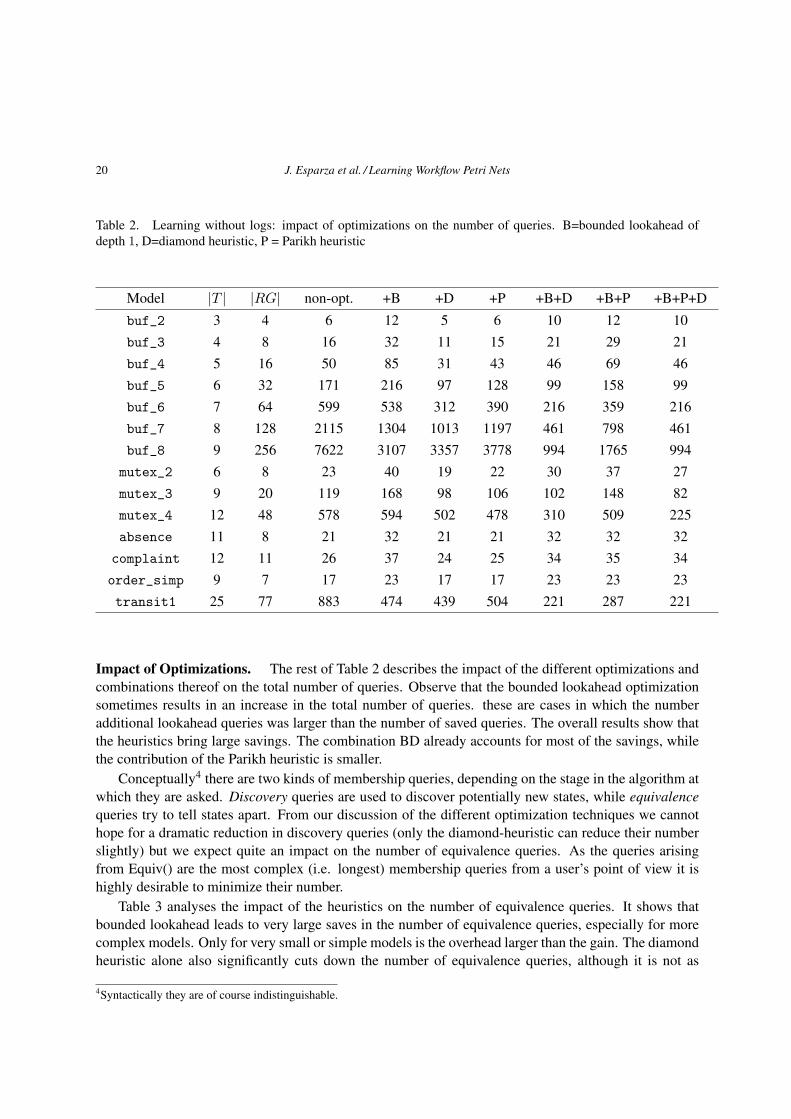
Table 3 analyses the impact of the heuristics on the number of equivalence queries. It shows that
bounded lookahead leads to very large saves in the number of equivalence queries, especially for more
complex models. Only for very small or simple models is the overhead larger than the gain. The diamond
heuristic alone also significantly cuts down the number of equivalence queries, although it is not as
4Syntactically they are of course indistinguishable.
J. Esparza et al. / Learning Workflow Petri Nets 21
Table 3. Learning without logs: number of calls to Equiv() with and without the optimizations, B=bounded
lookahead of depth 1, D=diamond heuristic, P=Parikh heuristic
Model non-opt. +B +D +P +B+D +B+P +B+P+D
buf_2 0 0 0 0 0 0 0
buf_3 3 1 2 2 0 0 0
buf_4 21 6 14 14 1 1 1
buf_5 106 19 64 63 2 2 2
buf_6 454 57 247 245 7 7 7
buf_7 1794 151 884 876 12 14 12
buf_8 6917 386 3100 3073 33 37 33
mutex_2 8 1 8 7 1 0 0
mutex_3 70 5 70 57 5 0 0
mutex_4 433 17 433 333 17 0 0
absence 9 3 9 9 3 3 3
complaint 11 3 10 10 2 2 2
order_simp 7 0 7 7 0 0 0
transit1 739 66 361 360 0 0 0
effective as the bounded lookahead. The Parikh and diamond heuristics have nearly the same effect on
the number of equivalence queries. Since moreover they both optimize in the same “direction”, their
combination is not too fruitful. Our main finding is that the combination of bounded lookahead and the
Parikh/diamond heuristic eliminates most of the calls to Equiv().
5.2.2. Learning with Initial Knowledge.
Our learning approach is not designed to replace workflow mining, but to complement the information
of incomplete logs. To analyse the effect of an existing log, we have generated random event logs for our
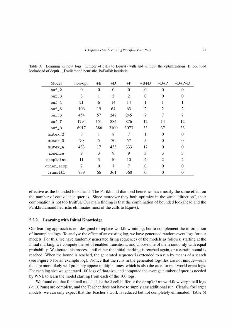
models. For this, we have randomly generated firing sequences of the models as follows: starting at the
initial marking, we compute the set of enabled transitions, and choose one of them randomly with equal
probability. We iterate this process until either the initial marking is reached again, or a certain bound is
reached. When the bound is reached, the generated sequence is extended to a run by means of a search
(see Figure 5 for an example log). Notice that the runs in the generated log-files are not unique—runs
that are more likely will probably appear multiple times, which is also the case for real-world event logs.
For each log size we generated 100 logs of that size, and computed the average number of queries needed
by WNL to learn the model starting from each of the 100 logs.
We found out that for small models like the 2-cell buffer or the complaint workflow very small logs
(< 10 runs) are complete, and the Teacher does not have to supply any additional run. Clearly, for larger
models, we can only expect that the Teacher’s work is reduced but not completely eliminated. Table 6)
22 J. Esparza et al. / Learning Workflow Petri Nets
.a.b.a.c.d.b.c.a.d.b.c.d.
.a.b.c.d.
.a.b.c.a.b.d.c.a.d.b.c.d.
.a.b.a.c.d.b.c.d.
.a.b.a.c.b.a.d.c.d.b.c.d.
.a.b.c.a.d.b.a.c.d.b.c.d.
.a.b.c.a.b.d.c.d.
.a.b.a.c.b.d.a.c.d.b.c.d.
.a.b.c.d.
.a.b.c.d.
a b c d
Figure 5. Example event log for 3-cell buffer
0
50
100
150
200
250
0 10 20 30 40 50 60 70 80 90 100
Ave
rage
num
. of q
uerie
s
Number of runs in log
buffer_5mutex_3mutex_4
transit
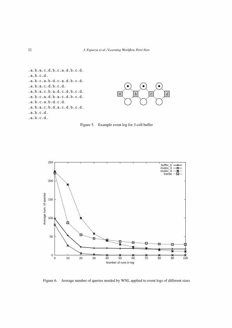
Figure 6. Average number of queries needed by WNL applied to event logs of different sizes
J. Esparza et al. / Learning Workflow Petri Nets 23
shows the reduction for the buf_5, mutex_3, mutex_4, and transit models as a function of the log
size. All optimizations described in Section 4 were employed for these tests.
We observe that small logs already reduce the number of queries to be answered quite drastically. At
the same time, because our logs may contain many identical entries, larger logs contribute less and less
new knowledge. This reflects the situation of real-life logs, which mostly contain common executions of
a workflow but lack less common runs.
The results depicted in Figures 2, 3 and 6 suggest that, despite the seemingly intimidating result in
Section 3.5, learning of workflow models is quite feasible for practical applications.
6. Conclusion
We have presented a new approach for mining workflow nets based on learning techniques. The approach
palliates the problem of incompleteness of event logs: if a log is incomplete, our algorithm derives
membership queries identifying the missing knowledge. The queries can be passed to an expert, whose
answers allow to produce a model.
We have shown the correctness and completeness of our approach given a teacher answering work-
flow membership queries. Starting with general combinatorial arguments showing that workflow models
can in principle be learned, we have derived a learning algorithm requiring a single exponential number
of queries in the worst case, and we have given a matching lower bound. We have also shown experimen-
tal evidence indicating that the combination of an event log, even of small size, and a Teacher responsible
for providing information on “corner cases” allows to efficiently produce models in practically relevant
cases.
There are several promising paths for further research. One aspect is the application of learning to
the design of workflows. In this approach an expert on business processes (the Teacher) and a modelling
expert (the Learner) cooperate. The Learner asks the Teacher queries about the expected behaviour of
the workflow, and proposes models. The models are criticized by the Teacher, who continues to ask
queries and refine the model until the Teacher is satisfied. The proposal of a model by the Learner and
its acceptance or rejection by the Teacher can be naturally modelled as an equivalence query (see the
discussion in Section 3.6). We expect to transfer ideas from the field of learning models of software
systems [13] to workflow systems, and develop “teaching assistants” that filter the queries, automatically
answering those for which the answer can be deduced from current information (for instance because it
is known that two tasks must be concurrent), and only passing to the expert the remaining ones. Here
we expect to profit from related work by Desel, Lorenz and others [12]. An important point for process
mining and even more for process design is designing fault tolerance techniques allowing to cope with
false answers by the Teacher. Finally, learning more general classes of Petri nets, and applications to
modelling/reconstruction of distributed systems, or biological/chemical processes, are also promising
paths for future work.
References
[1] van der Aalst, W., van Hee, K.: Workflow Management. Models, Methods, and Systems., MIT Press, 2004.
[2] van der Aalst, W. M. P.: The Application of Petri Nets to Workflow Management, Journal of Circuits,
Systems, and Computers, 8(1), 1998, 21–66.
24 J. Esparza et al. / Learning Workflow Petri Nets
[3] van der Aalst, W. M. P., van Dongen, B. F., Gunther, C. W., Mans, R. S., de Medeiros, A. K. A., Rozinat, A.,
Rubin, V., Song, M., Verbeek, H. M. W. E., Weijters, A. J. M. M.: ProM 4.0: Comprehensive Support for eal
Process Analysis, ICATPN, 2007.
[4] van der Aalst, W. M. P., van Dongen, B. F., Herbst, J., Maruster, L., Schimm, G., Weijters, A. J. M. M.:
Workflow mining: A survey of issues and approaches, Data Knowl. Eng., 47(2), 2003, 237–267.
[5] Agrawal, R., Gunopulos, D., Leymann, F.: Mining Process Models from Workflow Logs, EDBT, 1998.
[6] Andersen, H. R.: An Introduction to Binary Decision Diagrams, Technical report, 1999.
[7] Angluin, D.: Learning Regular Sets from Queries and Counterexamples, Information and Computation,
75(2), 1987, 87–106, ISSN 0890-5401.
[8] Badouel, E., Bernardinello, L., Darondeau, P.: Polynomial Algorithms for the Synthesis of Bounded Nets,
TAPSOFT ’95: Proceedings of the 6th International Joint Conference CAAP/FASE on Theory and Practice
of Software Development, Springer-Verlag, London, UK, 1995, ISBN 3-540-59293-8.
[9] Badouel, E., Darondeau, P.: On the synthesis of general Petri nets, Technical report, INRIA, 1996.
[10] Bergenthum, R., Desel, J., Kolbl, C., Mauser, S.: Experimental results on process mining based on regions
of languages, CHINA 2008, workshop at the Applications and theory of Petri nets : 29th international
conference, 2008.
[11] Bergenthum, R., Desel, J., Lorenz, R., Mauser, S.: Process Mining Based on Regions of Languages, BPM,
2007.
[12] Bergenthum, R., Desel, J., Mauser, S., Lorenz, R.: Construction of Process Models from Example Runs, T.
Petri Nets and Other Models of Concurrency, 2, 2009, 243–259.
[13] Bollig, B., Katoen, J.-P., Kern, C., Leucker, M.: Learning Communicating Automata from MSCs, IEEE
Transactions on Software Engineering (TSE), 36(3), May/June 2010, 390–408.
[14] Bollig, B., Katoen, J.-P., Kern, C., Leucker, M., Neider, D., Piegdon, D.: libalf: the Automata Learning
Framework, Proceedings of the 22nd International Conference on Computer-Aided Verification (CAV’10),
6174, Springer, 2010.
[15] Chow, T. S.: Testing Software Design Modeled by Finite-State Machines, TSE, 4(3), May 1978, 178–187,
Special collection based on COMPSAC.
[16] Kindler, E., Rubin, V., Schafer, W.: Process Mining and Petri Net Synthesis, Business Process Management
Workshops, 2006.
[17] Rubin, V., Gunther, C. W., van der Aalst, W. M. P., Kindler, E., van Dongen, B. F., Schafer, W.: Process
Mining Framework for Software Processes, ICSP, 2007.
[18] SAP AG: SAP Business Workflow Demo Examples (BC-BMT-WFM), 2001.
[19] Vasilevski, M. P.: Failure Diagnosis of Automata, Cybernetic, 9(4), 1973, 653–665.
[20] Verbeek, H. M.: Verification of WF-nets, Ph.D. Thesis, Technische Universiteit Eindhoven, 2004.