Learning Transportation Mode from Raw GPS Data for Geographic Applications on the Web

Yu Zheng, Like Liu, Longhao Wang, Xing Xie

Microsoft Research Asia 4F, Sigma building, No.49 Zhichun road, Haidian District, Beijing 100080, P. R. China

{yuzheng, v-liliu, v-lowang, xingx}@microsoft.com

ABSTRACT

Geographic information has spawned many novel Web

applications where global positioning system (GPS) plays

important roles in bridging the applications and end users.

Learning knowledge from users’ raw GPS data can provide rich

context information for both geographic and mobile applications.

However, so far, raw GPS data are still used directly without

much understanding. In this paper, an approach based on

supervised learning is proposed to automatically infer

transportation mode from raw GPS data. The transportation mode,

such as walking, driving, etc., implied in a user’s GPS data can

provide us valuable knowledge to understand the user. It also

enables context-aware computing based on user’s present

transportation mode and design of an innovative user interface for

Web users. Our approach consists of three parts: a change point-

based segmentation method, an inference model and a post-

processing algorithm based on conditional probability. The

change point-based segmentation method was compared with two

baselines including uniform duration based and uniform length

based methods. Meanwhile, four different inference models

including Decision Tree, Bayesian Net, Support Vector Machine

(SVM) and Conditional Random Field (CRF) are studied in the

experiments. We evaluated the approach using the GPS data

collected by 45 users over six months period. As a result, beyond

other two segmentation methods, the change point based method

achieved a higher degree of accuracy in predicting transportation

modes and detecting transitions between them. Decision Tree

outperformed other inference models over the change point based

segmentation method.

Categories and Subject Descriptors

H.4.3 [Information System Application]: Communications

Applications – Information browsers. H.5.2 [Information

Interface and Presentation]: User Interface. I.5.2 [Pattern

Recognition]: Design Methodology - Classifier design and

evaluation.

General Terms

Algorithm, Design, Experimentation.

Keywords

Geographic Applications, GPS, Transportation Mode, Machine

Learning, Classification.

1. INTRODUCTION In recent years, on the World Wide Web, geographic information

has enabled an explosion of applications in which locality and

mobility usually connect to one another closely. Web-based

mapping applications like Google Maps, Yahoo Maps and Live

Maps as well as mobile/local search engines have attracted

considerable interest among Web users and developers.

Meanwhile, with the increasing prevalence of GPS devices, as

never before, many communities that engaged in geographically

related activities have been established. For instance, GPS track

visualization and sharing over Web maps [1, 2, 3, 4, 5] as well as

geo-tagging photos for archiving and browsing [6] have been

incubated. In these applications, GPS data have played important

roles in bridging them and end users, e.g., ranking the results of

mobile/local search, tagging photos with locations, etc. However,

to date, most of these applications only use raw GPS data like

GPS coordinates and timestamps without much understanding,

while other applications needs support from manual efforts.

Neither method is optimal for the development of geographic and

mobile applications. In this paper, we aim to improve local/mobile

applications on the Web and enhance their connections by mining

knowledge from raw GPS data with minimal user efforts.

As a kind of knowledge mined from raw GPS data, transportation

modes such as walking, driving etc, and the transitions between

them are valuable for both users and application systems.

For users: The information helps individuals effectively

reflect on their past events and deeply understand their own

life pattern as well. Also, it presents richer knowledge over

the plain GPS tracks to other users and facilitates life sharing

among people.

For the application systems: 1) It enables context-aware

computing based on a user’s present transportation mode and

design of innovative web user interface. 2) It empowers the

application systems to distinguish GPS tracks by

transportation modes so that users can find proper routes to

their destinations in a more effective manner. 3) It allows the

systems to mine deeper knowledge such as traffic condition,

popular routes for different transportation modes, etc., from

public GPS data. Moreover, in many research [7][8][9][10][11][12] aiming to

understand user behavior from raw GPS data, transportation

mode is also important knowledge to support their work. It

can be used to improve the accuracy of prediction on an

individual’s outdoor movements. Also, it can contribute to

extract a user’s life pattern and discover the social pattern. In

turn, all the knowledge learned from this work can be

leveraged to enhance many innovative local/mobile

applications on the Web further.

However, due to the following two reasons, it is not feasible to

require every user to manually tag corresponding transportation

modes to their GPS tracks. 1) No motivation: Users cannot

directly achieve benefits from labeling their trips. 2) Difficulty: A

personal trip usually includes different transportation modes.

However, it is difficult for people to remember the accurate time

when they change their transportation modes.

Copyright is held by the International World Wide Web Conference

Committee (IW3C2). Distribution of these papers is limited to classroom

use, and personal use by others.

WWW 2008, April 21-25, 2008, Beijing, China.

ACM 978-1-60558-085-2/08/04.

On the other hand, the identification methods based on simple rule

like velocity-based approach, cannot handle this problem with

great effect. The features of different transportation modes are

usually vulnerable to traffic conditions and weather. Intuitively, in

congestion, the mean velocity of driving would be as slow as

walking while on a rainy day a bus may move more like a bike

from the perspective of velocity. When a user takes more than one

kind of transportation modes along a trip, the identification on

transportation mode becomes more difficult. Thus, we do need an

approach to automatically and accurately infer transportation

modes as well as the transitions between them from raw GPS data.

Meanwhile, to make the approach more general and universal, we

do not expect it relies on the data collected by other sensors like

cell-phone, Wi-Fi, RFID, and/or other information extracted from

geographic maps, such as road networks etc. In other words, the

inference approach should only depend on raw GPS data. To the

best of our knowledge, no related work solves this problem.

In this paper, for geographic and mobile applications on the Web,

we propose an approach using raw GPS data that is based on

supervised learning to automatically learn the transportation

modes including walking, taking a bus, riding a bike and driving.

The contributions of the work lie in that:

It is an important step towards improving geographic

applications on the Web by using knowledge mined from

raw GPS data.

Such knowledge can enhance the connection between

locality and mobility, and enable more novel applications on

the Web.

It helps users deeply understand their own experience and

better shares other people’s knowledge.

It enables local/mobile application systems to perform

context-aware computing based on transportation mode and

create an innovative user interface for Web users.

The advantages of our approach lie in that: 1) our approach can

infer compound trips, which contain more than one kind of

transportation modes. In addition, it can correctly detect the

transition between different transportation modes. 2) The

approach is independent of other information from maps and other

sensors. 3) The model learned from the dataset of some users can

be applied to infer GPS data from others.

The rest parts of the paper are organized as follows. First in

Section 2, we briefly introduce the architecture and the prototype

of GeoLife where our approach has been deployed to play

important roles. The significance of inferring transportation mode

is justified by three application scenarios here. Then, the

framework of our approach is described in Section 3 while the

detail methodologies are given in Section 4. Subsequently, in

Section 5, we evaluate our approach based on the GPS data from

45 people over a period of six months. Some experiments results

and corresponding discussions are also presented. Finally, after

introducing some related work in Section 6, we draw conclusions

and offer an outlook for our future work in Section 7.

2. GEOLIFE The work reported in this paper is a part of research into our

project GeoLife, which is a GPS-log-driven application over Web

Map. It focuses on lively visualization, effective organization, fast

retrieval and deeply understanding of GPS track logs for both

personal and public use.

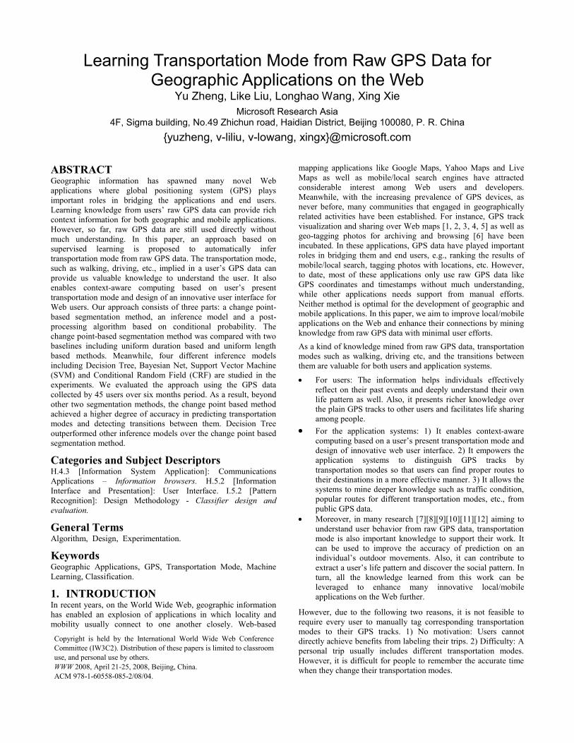
As shown in Figure 1, given the GPS track log as well as

associated multimedia data people created in their daily lives,

GeoLife helps users visualize their past events on Web maps and

understand their personal life pattern as well. By publishing some

of GPS tracks out, users can share life experience with others and

absorb rich knowledge from others’ GPS tracks. Based on public

data, more knowledge such as popular travel routes, hot places

and traffic condition, etc., can be mined. The mined knowledge

can be recommended to users via Web or mobile user interface

(UI) when they need suggestions. Further, a spatial-temporal

search function, which allows users to give a spatial range over

maps and/or temporal interval as a query, is offered in GeoLife to

help people effectively find out the GPS tracks they are interested

in. The search function does not only facilitates allowing people

to efficiently get information from other’s life experience but also

support each person’s recall of past events.

Indexing

Recommendation

….….…...….….…...

Spatial-Temporal

Index

Route SearchData Pre-Process

GPS Data Mining

Public Knowledge Personal Knowledge

GPS/

Multimedia

Data

GPS Log File

Visualization

Personal

Archive

Video

Multimedia Files

Image Audio

UploadUsers

Web UI Mobile UI

GPS

Phone

Figure 1. Architecture of GeoLife

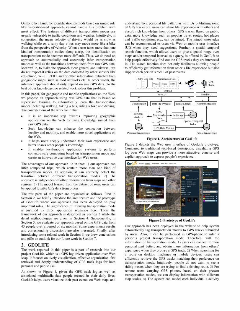
Figure 2 depicts the Web user interface of GeoLife prototype.

Compared to traditional text-based description, visualizing GPS

log over Web maps can provide a more attractive, concise and

explicit approach to express people’s experience.

Figure 2. Prototype of GeoLife

Our approach has been deployed in the website to help system

automatically tag transportation modes to GPS tracks submitted

by users. Also, it can be performed in GPS-phone to infer a

person’s present transportation mode. Therefore, with the

information of transportation mode, 1) users can connect to their

personal past better, and obtain more information from others’

experience when they browse a GPS track. 2) When searching for

a route on desktop machines or mobile devices, users can

efficiently retrieve the GPS tracks matching their preference on

transportation mode. Intuitively, people do not want to see a

riding means when they are trying to find a driving route. 3) For

remote users carrying GPS phones, based on their present

transportation modes, we can display information with different

map scales. 4) The system can model each individual’s activity

more accurately and delivery commonsense information, e.g. bus

schedules, in advance.

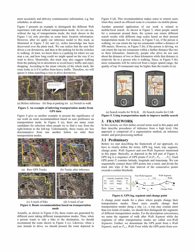
Figure 3 presents an example to distinguish the different Web

experience with and without transportation mode. As we can see,

without the tag of transportation mode, the track shown in the

Figure 3 (a) only provides us some basic location information.

However, after we apply our inference model to this track, as

illustrated in Figure 3 (b) and (c), richer knowledge has been

discovered over the plain track. We can realize that the user first

drives a car downtown, and then at the parking lot he/she switches

to walking. At least, we know there is a parking lot where we can

stop a car, and how long could we might spend on the way if we

want to drive. Meanwhile, this track may also suggest walking

from the parking lot to downtown to avoid heavy traffic and enjoy

shopping. According to the mean velocity of the whole track, the

route looks as it if it suffers from heavy traffic. Therefore, we will

ignore it when searching a way to drive downtown.

(a) Before inference (b) Stop at parking lot (c) Switch to walk

Figure 3. An example of inferring transportation modes from

GPS data

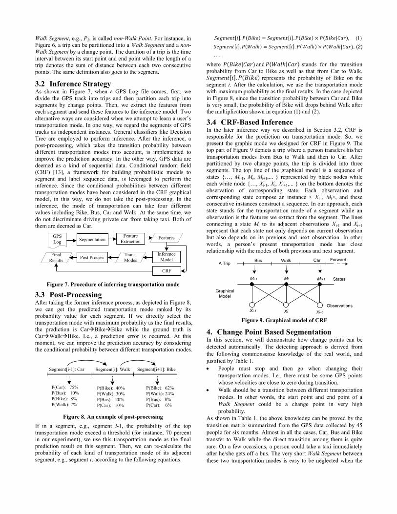
Figure 4 give us another example to present the significance of

our work on route recommendation based on user preference on

transportation mode. In Figure 4 (a), there are many route

candidates for selection when people try to find a way from the

right-bottom to the left-top. Unfortunately, these routes are less

discriminative from one another before we infer their

transportation modes.

(a) Raw GPS Tracks (b) Tracks after inference

(c) A track of bike (d) A track of car

Figure 4. Route recommendation based on transportation

mode

Actually, as shown in Figure 4 (b), these routes are generated by

different users taking different transportation modes. Thus, when

a person wants to ride a bike to the destination, we should

recommend the route shown in Figure 4 (c). Likewise, when a

user intends to drive, we should present the route depicted in

Figure 4 (d). This recommendation makes sense to remote users

when they search an efficient route to a location via mobile phone.

Another potential application of our work is related to

mobile/local search. As shown in Figure 5, when people search

for a restaurant around them, the system can return different

search results with different map scales based on their present

transportation mode. For instance, in Figure 5 (a), if the person is

walking, we can return the top ten restaurants within a distance of

500 meters. However, in Figure 5 (b), if the person is driving, we

can return the top ten restaurants within a farther distance like two

or three kilometers. Intuitively, people who drive do not care

about the distance of two or three kilometers while that distance is

relatively far to a person who is walking. Since, in Figure 5 (b),

more restaurants will be retrieved from a larger spatial range, the

quality of top 10 restaurants may be higher than the results in (a).

(a) Search results for WALK (b) Search results for CAR

Figure 5. Using transportation mode to improve mobile search

3. FRAMEWORK In this section, we first define several terms used in this paper and

then describe procedures of inference from a high level. Our

approach is comprised of a segmentation method, an inference

model, and post-processing method.

3.1 Preliminary Before we start describing the framework of our approach, we

have to clearly define the terms, GPS log, track, trip, segment,

change point, Walk Segment and non-Walk Segments mentioned

in this paper. Basically, as depicted in the left part of Figure 6,

GPS log is a sequence of GPS points Pi ∈{P1, P2, … , Pn}. Each

GPS point Pi contains latitude, longitude and timestamp. We can

sequentially connect these GPS points into a track, and divide the

track into trips if the time interval of the consecutive points

exceeds a certain threshold.

Latitude, longitude, Time

P1: Lat1, long1, T1

P2: Lat2, long2, T2

………...

Pn: Latn, longn, Tn

P1

Pn

Car

P2 P3 Pn-1

Change Point

WalkNon-Walk Segment

L1L2

Walk Segment

Figure 6. GPS log, segment and change point

A change point stands for a place where people change their

transportation modes. Since users usually change their

transportation modes along a trip, i.e., a trip may contain more

than two kinds of modes, we should first distinguish the segments

of different transportation modes. For the description convenience,

we name the segment of walk after Walk Segment while the

segments of other transportation modes are called non-Walk

Segments. Further, we denominate the GPS point from a Walk

Segment, such as Pn-1, Walk Point while the GPS point from non-

Walk Segment, e.g., P2, is called non-Walk Point. For instance, in

Figure 6, a trip can be partitioned into a Walk Segment and a non-

Walk Segment by a change point. The duration of a trip is the time

interval between its start point and end point while the length of a

trip denotes the sum of distance between each two consecutive

points. The same definition also goes to the segment.

3.2 Inference Strategy As shown in Figure 7, when a GPS Log file comes, first, we

divide the GPS track into trips and then partition each trip into

segments by change points. Then, we extract the features from

each segment and send these features to the inference model. Two

alternative ways are considered when we attempt to learn a user’s

transportation mode. In one way, we regard the segments of GPS

tracks as independent instances. General classifiers like Decision

Tree are employed to perform inference. After the inference, a

post-processing, which takes the transition probability between

different transportation modes into account, is implemented to

improve the prediction accuracy. In the other way, GPS data are

deemed as a kind of sequential data. Conditional random field

(CRF) [13], a framework for building probabilistic models to

segment and label sequence data, is leveraged to perform the

inference. Since the conditional probabilities between different

transportation modes have been considered in the CRF graphical

model, in this way, we do not take the post-processing. In the

inference, the mode of transportation can take four different

values including Bike, Bus, Car and Walk. At the same time, we

do not discriminate driving private car from taking taxi. Both of

them are deemed as Car.

Figure 7. Procedure of inferring transportation mode

3.3 Post-Processing After taking the former inference process, as depicted in Figure 8,

we can get the predicted transportation mode ranked by its

probability value for each segment. If we directly select the

transportation mode with maximum probability as the final results,

the prediction is CarBikeBike while the ground truth is

CarWalkBike. I.e., a prediction error is occurred. At this

moment, we can improve the prediction accuracy by considering

the conditional probability between different transportation modes.

Segment[i-1]: Car Segment[i]: Walk Segment[i+1]: Bike

P(Car): 75%

P(Bus): 10%

P(Bike): 8%

P(Walk): 7%

P(Bike): 62%

P(Walk): 24%

P(Bus): 8%

P(Car): 6%

P(Bike): 40%

P(Walk): 30%

P(Bus): 20%

P(Car): 10%

Figure 8. An example of post-processing

If in a segment, e.g., segment i-1, the probability of the top

transportation mode exceed a threshold (for instance, 70 percent

in our experiment), we use this transportation mode as the final

prediction result on this segment. Then, we can re-calculate the

probability of each kind of transportation mode of its adjacent

segment, e.g., segment i, according to the following equations.

𝑆𝑒𝑔𝑚𝑒𝑛𝑡 𝑖 . 𝑃 𝐵𝑖𝑘𝑒 = 𝑆𝑒𝑔𝑚𝑒𝑛𝑡 𝑖 . 𝑃 𝐵𝑖𝑘𝑒 × 𝑃 𝐵𝑖𝑘𝑒 𝐶𝑎𝑟 , (1)

𝑆𝑒𝑔𝑚𝑒𝑛𝑡 𝑖 . 𝑃 𝑊𝑎𝑙𝑘 = 𝑆𝑒𝑔𝑚𝑒𝑛𝑡 𝑖 . 𝑃 𝑊𝑎𝑙𝑘 × 𝑃(𝑊𝑎𝑙𝑘|𝐶𝑎𝑟), (2)

….

where 𝑃(𝐵𝑖𝑘𝑒|𝐶𝑎𝑟) and 𝑃 𝑊𝑎𝑙𝑘 𝐶𝑎𝑟 stands for the transition

probability from Car to Bike as well as that from Car to Walk.

𝑆𝑒𝑔𝑚𝑒𝑛𝑡 𝑖 . 𝑃 𝐵𝑖𝑘𝑒 represents the probability of Bike on the

segment i. After the calculation, we use the transportation mode

with maximum probability as the final results. In the case depicted

in Figure 8, since the transition probability between Car and Bike

is very small, the probability of Bike will drops behind Walk after

the multiplication shown in equation (1) and (2).

3.4 CRF-Based Inference In the later inference way we described in Section 3.2, CRF is

responsible for the prediction on transportation mode. So, we

present the graphic mode we designed for CRF in Figure 9. The

top part of Figure 9 depicts a trip where a person transfers his/her

transportation modes from Bus to Walk and then to Car. After

partitioned by two change points, the trip is divided into three

segments. The top line of the graphical model is a sequence of

states {…, Mi-1, Mi, Mi+1,... } represented by black nodes while

each white node {…, Xi-1, Xi, Xi+1,... } on the bottom denotes the

observation of corresponding state. Each observation and

corresponding state compose an instance < Xi , Mi>, and these

consecutive instances construct a sequence. In our approach, each

state stands for the transportation mode of a segment while an

observation is the features we extract from the segment. The lines

connecting a state Mi to its adjacent observations Xi-1 and Xi+1

represent that each state not only depends on current observation

but also depends on its previous and next observation. In other

words, a person’s present transportation mode has close

relationship with the modes of both previous and next segment.

Mi-1 Mi Mi+1

Xi-1 Xi Xi+1

Observations

States

WalkBus ForwardCar

Graphical

Model

A Trip

Figure 9. Graphical model of CRF

4. Change Point Based Segmentation In this section, we will demonstrate how change points can be

detected automatically. The detecting approach is derived from

the following commonsense knowledge of the real world, and

justified by Table 1.

People must stop and then go when changing their

transportation modes. I.e., there must be some GPS points

whose velocities are close to zero during transition.

Walk should be a transition between different transportation

modes. In other words, the start point and end point of a

Walk Segment could be a change point in very high

probability.

As shown in Table 1, the above knowledge can be proved by the

transition matrix summarized from the GPS data collected by 45

people for six months. Almost in all the cases, Car, Bus and Bike

transfer to Walk while the direct transition among them is quite

rare. On a few occasions, a person could take a taxi immediately

after he/she gets off a bus. The very short Walk Segment between

these two transportation modes is easy to be neglected when the

Inference

ModelPost Process

GPS

LogSegmentation

Feature

ExtractionFeatures

Trans.

Modes

Final

Results

CRF

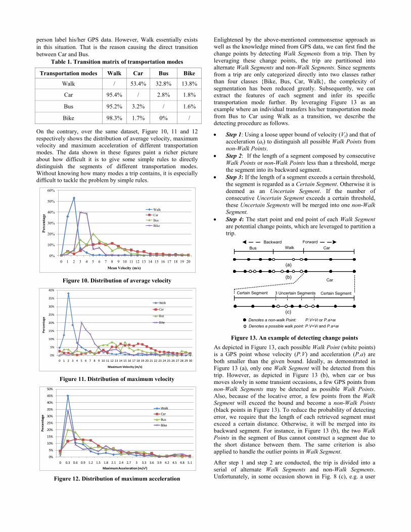
person label his/her GPS data. However, Walk essentially exists

in this situation. That is the reason causing the direct transition

between Car and Bus. Table 1. Transition matrix of transportation modes

Transportation modes Walk Car Bus Bike

Walk / 53.4% 32.8% 13.8%

Car 95.4% / 2.8% 1.8%

Bus 95.2% 3.2% / 1.6%

Bike 98.3% 1.7% 0% /

On the contrary, over the same dataset, Figure 10, 11 and 12

respectively shows the distribution of average velocity, maximum

velocity and maximum acceleration of different transportation

modes. The data shown in these figures paint a richer picture

about how difficult it is to give some simple rules to directly

distinguish the segments of different transportation modes.

Without knowing how many modes a trip contains, it is especially

difficult to tackle the problem by simple rules.

Figure 10. Distribution of average velocity

Figure 11. Distribution of maximum velocity

Figure 12. Distribution of maximum acceleration

Enlightened by the above-mentioned commonsense approach as

well as the knowledge mined from GPS data, we can first find the

change points by detecting Walk Segments from a trip. Then by

leveraging these change points, the trip are partitioned into

alternate Walk Segments and non-Walk Segments. Since segments

from a trip are only categorized directly into two classes rather

than four classes {Bike, Bus, Car, Walk}, the complexity of

segmentation has been reduced greatly. Subsequently, we can

extract the features of each segment and infer its specific

transportation mode further. By leveraging Figure 13 as an

example where an individual transfers his/her transportation mode

from Bus to Car using Walk as a transition, we describe the

detecting procedure as follows.

Step 1: Using a loose upper bound of velocity (Vt) and that of

acceleration (at) to distinguish all possible Walk Points from

non-Walk Points.

Step 2: If the length of a segment composed by consecutive

Walk Points or non-Walk Points less than a threshold, merge

the segment into its backward segment.

Step 3: If the length of a segment exceeds a certain threshold,

the segment is regarded as a Certain Segment. Otherwise it is

deemed as an Uncertain Segment. If the number of

consecutive Uncertain Segment exceeds a certain threshold,

these Uncertain Segments will be merged into one non-Walk

Segment.

Step 4: The start point and end point of each Walk Segment

are potential change points, which are leveraged to partition a

trip.

WalkBus

Certain Segment

Denotes a non-walk Point: P.V>Vt or P.a>at

Denotes a possible walk point: P.V<Vt and P.a<at

(b)

(c)

Backward Forward

Car

(a)

Certain Segment3 Uncertain Segments

Car

Figure 13. An example of detecting change points

As depicted in Figure 13, each possible Walk Point (white points)

is a GPS point whose velocity (P.V) and acceleration (P.a) are

both smaller than the given bound. Ideally, as demonstrated in

Figure 13 (a), only one Walk Segment will be detected from this

trip. However, as depicted in Figure 13 (b), when car or bus

moves slowly in some transient occasions, a few GPS points from

non-Walk Segments may be detected as possible Walk Points.

Also, because of the locative error, a few points from the Walk

Segment will exceed the bound and become a non-Walk Points

(black points in Figure 13). To reduce the probability of detecting

error, we require that the length of each retrieved segment must

exceed a certain distance. Otherwise, it will be merged into its

backward segment. For instance, in Figure 13 (b), the two Walk

Points in the segment of Bus cannot construct a segment due to

the short distance between them. The same criterion is also

applied to handle the outlier points in Walk Segment.

After step 1 and step 2 are conducted, the trip is divided into a

serial of alternate Walk Segments and non-Walk Segments.

Unfortunately, in some occasion shown in Fig. 8 (c), e.g. a user

0%

10%

20%

30%

40%

50%

60%

0 1 2 3 4 5 6 7 8 9 10 11 12 13 14 15 16 17 18 19 20

Per

cen

tage

Mean Velocity (m/s)

Walk

Car

Bus

Bike

0%

5%

10%

15%

20%

25%

30%

35%

40%

0 1 2 3 4 5 6 7 8 9 10 11 12 13 14 15 16 17 18 19 20 21 22 23 24 25 26 27 28 29 30

Per

cen

tage

Maximum Velocity (m/s)

Walk

Car

Bus

Bike

0%

5%

10%

15%

20%

25%

30%

35%

40%

45%

50%

0 0.3 0.6 0.9 1.2 1.5 1.8 2.1 2.4 2.7 3 3.3 3.6 3.9 4.2 4.5 4.8 5.1

Pe

rce

nta

ge

Maximum Acceleration (m/s2)

Walk

Car

Bus

Bike

meets a congestion or heavy traffic, a segment of car may be

comprised of many alternate Walk Segments and non-Walk

Segments after detection. It is not appropriate for the inference

model to directly predict their transportation modes over the

features extracted from such segments. It is commonsense that the

longer a segment is, the richer features of its transportation mode

a segment will express. Hence, it is more probable for us to infer

its transportation mode correctly. On the contrary, the shorter a

segment is, the higher the uncertainty is. To avoid the incorrect

partition which will lead to the further inference error, we take the

following policy to merge, to some extent, the consecutive

Uncertain Segments. We define a segment whose length exceeds a

threshold (e.g., fifty meters used in the experiments) as a Certain

Segment. Otherwise, we deem it as an Uncertain Segment. I.e., we

are not sure about the transportation mode of this segment even if

it holds the condition of a Walk Segment. If the number of

consecutive Uncertain Segments exceeds a certain threshold, e.g.,

three we find out in experiments, we still deem all these Uncertain

Segments as one non-Walk Segments. It is not difficult to

understand that common users will not frequently change their

transportation modes within such a short distance. For instance, as

depicted in Figure 13 (c), within a certain distance, it is

impossible for a person to take the following transition, Car

Walk Car Walk Car. So, we believe the middle three

segments between the two Certain Segments are also non-Walk

Segments, Car here. Thus, we can merge the three Uncertain

Segments into one segment and perform the further inference.

5. EXPERIMENTS In this section, at first, we describe the framework of the

experiment. The setup includes GPS data, toolkits and parameters

of each algorithm we used in our experiments are presented

respectively. Subsequently, detailed experimental results are given.

Finally, corresponding discussions are provided based on the

evaluation results.

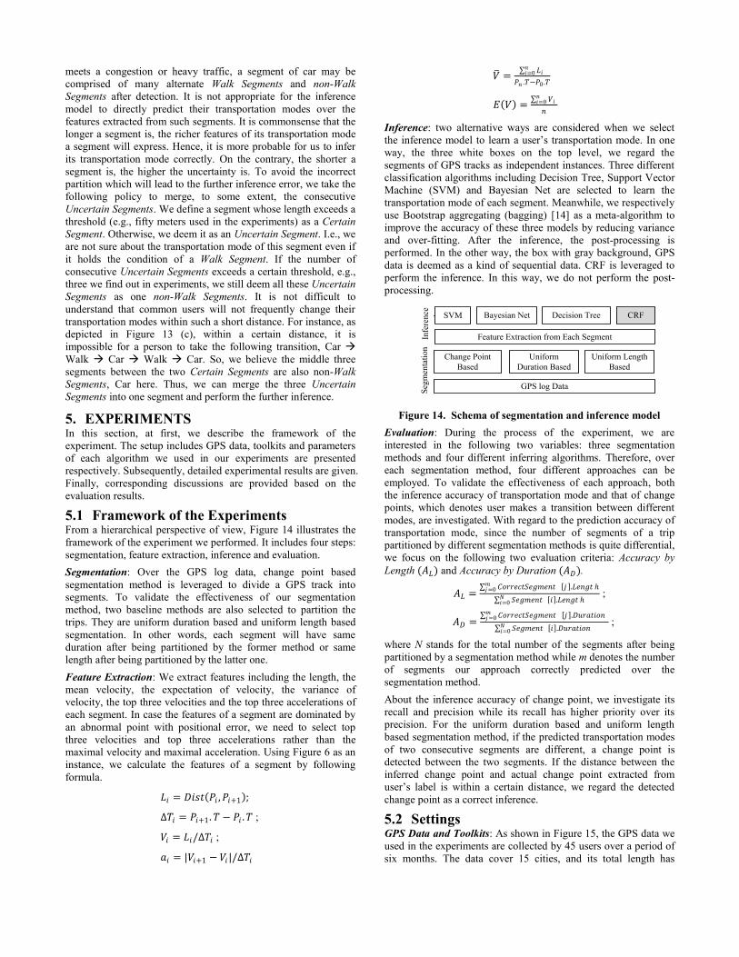
5.1 Framework of the Experiments From a hierarchical perspective of view, Figure 14 illustrates the

framework of the experiment we performed. It includes four steps:

segmentation, feature extraction, inference and evaluation.

Segmentation: Over the GPS log data, change point based

segmentation method is leveraged to divide a GPS track into

segments. To validate the effectiveness of our segmentation

method, two baseline methods are also selected to partition the

trips. They are uniform duration based and uniform length based

segmentation. In other words, each segment will have same

duration after being partitioned by the former method or same

length after being partitioned by the latter one.

Feature Extraction: We extract features including the length, the

mean velocity, the expectation of velocity, the variance of

velocity, the top three velocities and the top three accelerations of

each segment. In case the features of a segment are dominated by

an abnormal point with positional error, we need to select top

three velocities and top three accelerations rather than the

maximal velocity and maximal acceleration. Using Figure 6 as an

instance, we calculate the features of a segment by following

formula.

𝐿𝑖 = 𝐷𝑖𝑠𝑡 𝑃𝑖 , 𝑃𝑖+1 ;

∆𝑇𝑖 = 𝑃𝑖+1. 𝑇 − 𝑃𝑖 . 𝑇 ;

𝑉𝑖 = 𝐿𝑖/∆𝑇𝑖 ;

𝑎𝑖 = |𝑉𝑖+1 − 𝑉𝑖|/∆𝑇𝑖

𝑉 = 𝐿𝑖

𝑛𝑖=0

𝑃𝑛 .𝑇−𝑃0 .𝑇

𝐸 𝑉 = 𝑉𝑖

𝑛𝑖=0

𝑛

Inference: two alternative ways are considered when we select

the inference model to learn a user’s transportation mode. In one

way, the three white boxes on the top level, we regard the

segments of GPS tracks as independent instances. Three different

classification algorithms including Decision Tree, Support Vector

Machine (SVM) and Bayesian Net are selected to learn the

transportation mode of each segment. Meanwhile, we respectively

use Bootstrap aggregating (bagging) [14] as a meta-algorithm to

improve the accuracy of these three models by reducing variance

and over-fitting. After the inference, the post-processing is

performed. In the other way, the box with gray background, GPS

data is deemed as a kind of sequential data. CRF is leveraged to

perform the inference. In this way, we do not perform the post-

processing.

GPS log Data

Change Point

Based

Uniform

Duration Based

Uniform Length

Based

Bayesian NetSVM Decision Tree CRF

Feature Extraction from Each Segment

Seg

men

tati

on

Infe

rence

Figure 14. Schema of segmentation and inference model

Evaluation: During the process of the experiment, we are

interested in the following two variables: three segmentation

methods and four different inferring algorithms. Therefore, over

each segmentation method, four different approaches can be

employed. To validate the effectiveness of each approach, both

the inference accuracy of transportation mode and that of change

points, which denotes user makes a transition between different

modes, are investigated. With regard to the prediction accuracy of

transportation mode, since the number of segments of a trip

partitioned by different segmentation methods is quite differential,

we focus on the following two evaluation criteria: Accuracy by

Length (𝐴𝐿) and Accuracy by Duration (𝐴𝐷).

𝐴𝐿 = 𝐶𝑜𝑟𝑟𝑒𝑐𝑡𝑆𝑒𝑔𝑚𝑒𝑛𝑡 𝑗 .𝐿𝑒𝑛𝑔𝑡 ℎ𝑚

𝑗=0

𝑆𝑒𝑔𝑚𝑒𝑛𝑡 𝑖 .𝐿𝑒𝑛𝑔𝑡 ℎ𝑁𝑖=0

;

𝐴𝐷 = 𝐶𝑜𝑟𝑟𝑒𝑐𝑡𝑆𝑒𝑔𝑚𝑒𝑛𝑡 𝑗 .𝐷𝑢𝑟𝑎𝑡𝑖𝑜𝑛𝑚

𝑗=0

𝑆𝑒𝑔𝑚𝑒𝑛𝑡 𝑖 .𝐷𝑢𝑟𝑎𝑡𝑖𝑜𝑛𝑁𝑖=0

;

where N stands for the total number of the segments after being

partitioned by a segmentation method while m denotes the number

of segments our approach correctly predicted over the

segmentation method.

About the inference accuracy of change point, we investigate its

recall and precision while its recall has higher priority over its

precision. For the uniform duration based and uniform length

based segmentation method, if the predicted transportation modes

of two consecutive segments are different, a change point is

detected between the two segments. If the distance between the

inferred change point and actual change point extracted from

user’s label is within a certain distance, we regard the detected

change point as a correct inference.

5.2 Settings GPS Data and Toolkits: As shown in Figure 15, the GPS data we

used in the experiments are collected by 45 users over a period of

six months. The data cover 15 cities, and its total length has

exceeded 20,000 kilometer. About 70 percent of the data are used

as a training set while the rest is used as test data. The GPS device

we chose to collect data from included handheld GPS receivers

(Magellan Explorist 210 or 300) and GPS phones. All the GPS

devices receive GPS coordinates every second and record a GPS

point once the velocity of a user changes to a certain extent or

his/her moving direction varies up to a threshold. After data

collection, we segment the track into trips if the interval between

two consecutive GPS points exceeds 20 minutes. Further, these

trips are partitioned into separate segments by the three

segmentation methods mentioned above. With regard to the

toolkit we used in the experiments, Weka 3.4 toolkit [14] is

selected to implement Decision Tree (REPTree), SVM/SMO

(linear) and Bayesian Net while CRF++ [15] are leveraged to

perform CRF algorithm over the partitioned segments.

Figure 15. GPS data and GPS devices

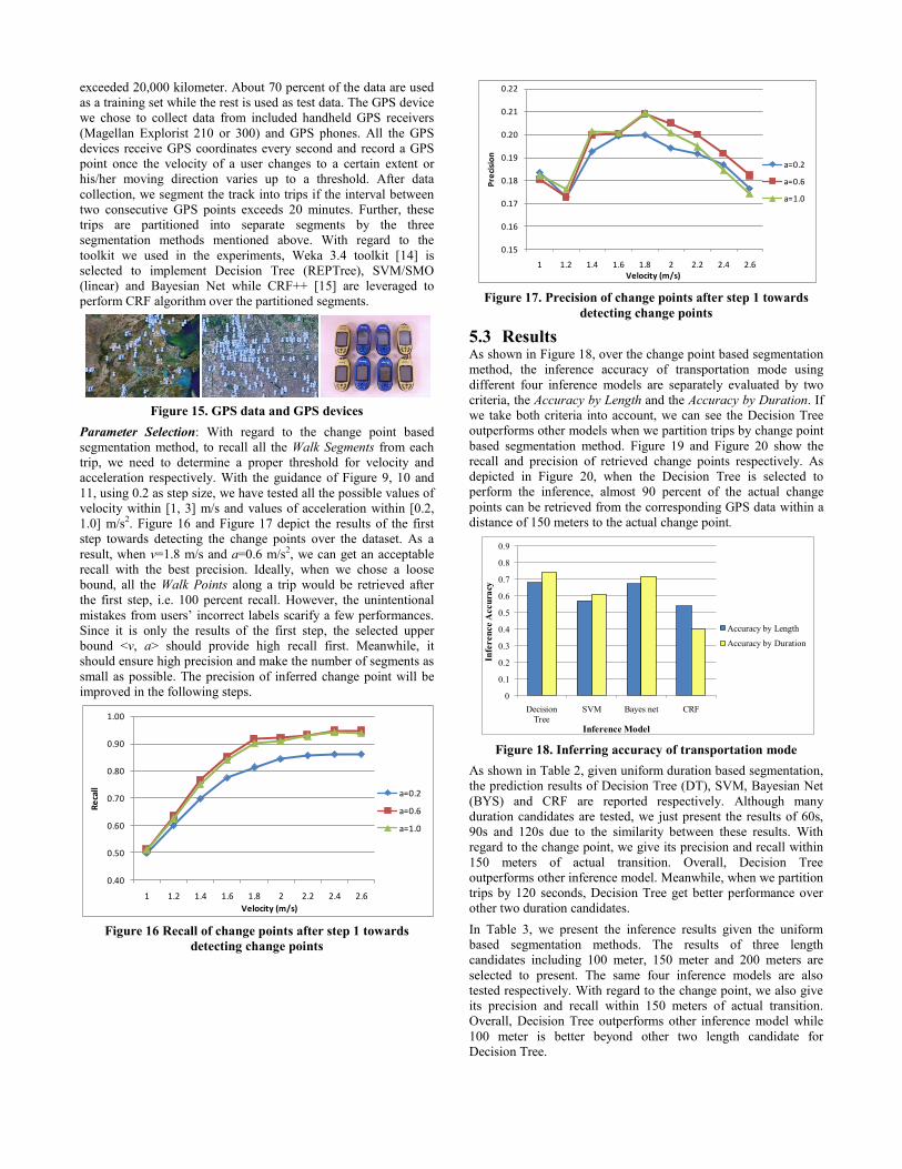
Parameter Selection: With regard to the change point based

segmentation method, to recall all the Walk Segments from each

trip, we need to determine a proper threshold for velocity and

acceleration respectively. With the guidance of Figure 9, 10 and

11, using 0.2 as step size, we have tested all the possible values of

velocity within [1, 3] m/s and values of acceleration within [0.2,

1.0] m/s2. Figure 16 and Figure 17 depict the results of the first

step towards detecting the change points over the dataset. As a

result, when v=1.8 m/s and a=0.6 m/s2, we can get an acceptable

recall with the best precision. Ideally, when we chose a loose

bound, all the Walk Points along a trip would be retrieved after

the first step, i.e. 100 percent recall. However, the unintentional

mistakes from users’ incorrect labels scarify a few performances.

Since it is only the results of the first step, the selected upper

bound <v, a> should provide high recall first. Meanwhile, it

should ensure high precision and make the number of segments as

small as possible. The precision of inferred change point will be

improved in the following steps.

Figure 16 Recall of change points after step 1 towards

detecting change points

Figure 17. Precision of change points after step 1 towards

detecting change points

5.3 Results As shown in Figure 18, over the change point based segmentation

method, the inference accuracy of transportation mode using

different four inference models are separately evaluated by two

criteria, the Accuracy by Length and the Accuracy by Duration. If

we take both criteria into account, we can see the Decision Tree

outperforms other models when we partition trips by change point

based segmentation method. Figure 19 and Figure 20 show the

recall and precision of retrieved change points respectively. As

depicted in Figure 20, when the Decision Tree is selected to

perform the inference, almost 90 percent of the actual change

points can be retrieved from the corresponding GPS data within a

distance of 150 meters to the actual change point.

Figure 18. Inferring accuracy of transportation mode

As shown in Table 2, given uniform duration based segmentation,

the prediction results of Decision Tree (DT), SVM, Bayesian Net

(BYS) and CRF are reported respectively. Although many

duration candidates are tested, we just present the results of 60s,

90s and 120s due to the similarity between these results. With

regard to the change point, we give its precision and recall within

150 meters of actual transition. Overall, Decision Tree

outperforms other inference model. Meanwhile, when we partition

trips by 120 seconds, Decision Tree get better performance over

other two duration candidates.

In Table 3, we present the inference results given the uniform

based segmentation methods. The results of three length

candidates including 100 meter, 150 meter and 200 meters are

selected to present. The same four inference models are also

tested respectively. With regard to the change point, we also give

its precision and recall within 150 meters of actual transition.

Overall, Decision Tree outperforms other inference model while

100 meter is better beyond other two length candidate for

Decision Tree.

0.40

0.50

0.60

0.70

0.80

0.90

1.00

1 1.2 1.4 1.6 1.8 2 2.2 2.4 2.6

Re

call

Velocity (m/s)

a=0.2

a=0.6

a=1.0

0.15

0.16

0.17

0.18

0.19

0.20

0.21

0.22

1 1.2 1.4 1.6 1.8 2 2.2 2.4 2.6

Pre

cisi

on

Velocity (m/s)

a=0.2

a=0.6

a=1.0

0

0.1

0.2

0.3

0.4

0.5

0.6

0.7

0.8

0.9

Decision

Tree

SVM Bayes net CRF

Infe

ren

ce A

ccu

racy

Inference Model

Accuracy by Length

Accuracy by Duration

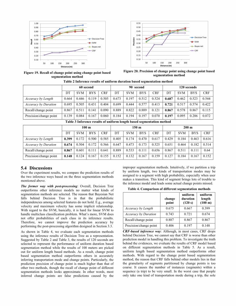
Figure 19. Recall of change point using change point based

segmentation method

Figure 20. Precision of change point using change point based

segmentation method

Table 2 Inference results of uniform duration based segmentation method

60 second 90 second 120 seconds

DT SVM BYS CRF DT SVM BYS CRF DT SVM BYS CRF

Accuracy by Length 0.664 0.446 0.119 0.505 0.673 0.197 0.512 0.524 0.687 0.462 0.523 0.544

Accuracy by Duration 0.695 0.505 0.431 0.404 0.699 0.444 0.577 0.413 0.721 0.517 0.574 0.422

Recall/change point 0.867 0.511 0.141 0.090 0.889 0.822 0.889 0.121 0.867 0.578 0.867 0.115

Precision/change point 0.139 0.084 0.167 0.060 0.184 0.194 0.197 0.070 0.197 0.095 0.206 0.072

Table 3 Inference results of uniform length based segmentation method

100 m 150 m 200 m

DT SVM BYS CRF DT SVM BYS CRF DT SVM BYS CRF

Accuracy by Length 0.399 0.172 0.500 0.585 0.405 0.174 0.470 0.617 0.429 0.184 0.463 0.616

Accuracy by Duration 0.674 0.504 0.172 0.566 0.647 0.473 0.173 0.525 0.651 0.464 0.182 0.514

Recall/change point 0.867 0.601 0.111 0.641 0.889 0.533 0.111 0.656 0.867 0.511 0.111 0.64

Precision/change point 0.148 0.124 0.167 0.155 0.152 0.132 0.167 0.159 0.127 0.184 0.167 0.152

5.4 Discussions Over the experiment results, we compare the prediction results of

the two inference ways based on the three segmentation methods

mentioned above.

The former way with post-processing: Overall, Decision Tree

outperforms other inference models no matter what kinds of

segmentation methods are selected. The reason that Bayesian Net

falls behind Decision Tree is in that the probabilistic

independencies among selected features do not hold. E.g., average

velocity and maximum velocity has some implicit relationship.

With regard to the SVM, basically, it is hard for linear SVM to

handle multiclass classification problem. What’s more, SVM does

not offer probabilities of each class in its inference results.

Therefore, we cannot improve the prediction accuracy by

performing the post-processing algorithm designed in Section 3.3.

As shown in Table 4, we evaluate each segmentation methods

using the inference results of Decision Tree as a representation.

Suggested by Table 2 and Table 3, the results of 120 seconds are

selected to represent the performance of uniform duration based

segmentation method while the results of 100 meters are picked

out for uniform length based methods. As a result, change point

based segmentation method outperforms others in accurately

inferring transportation mode and change points. Particularly, the

prediction precision of change point is much higher than that of

other two methods, though the recall of change point of different

segmentation methods looks approximate. In other words, most

inferred change points are false predictions caused by the

improper segmentation methods. Intuitively, if we partition a trip

by uniform length, two kinds of transportation modes may be

assigned to a segment with high probability, especially when user

makes a transition. This kind of segment brings lots of trouble to

the inference model and leads some actual change points missed.

Table 4. Comparison of different segmentation methods

change

point

uniform

duration

(120 s)

uniform

length

(100 m)

Accuracy by Length 0.675 0.667 0.399

Accuracy by Duration 0.743 0.721 0.674

Recall/change point 0.887 0.867 0.867

Precision/change point 0.406 0.197 0.148

CRF-based inference way: Although, in most cases, CRF drops

behind Decision Tree, we cannot say that CRF is worse than other

prediction model in handling this problem. To investigate the truth

behind the evidences, we evaluate the results of CRF model based

on different segmentation methods in Table 5. As a result,

uniform length based segmentation method outperforms other

methods. With regard to the change point based segmentation

method, the reason that CRF falls behind other models lies in that

the granularity of segments partitioned by change points is too

coarse. It causes the number of instances (segments) within a

sequence (a trip) to be very small. In the worst case that people

only take one kind of transportation mode during a trip, the sole

0.10

0.20

0.30

0.40

0.50

0.60

0.70

0.80

0.90

1.00

50 100 150 200 250 300

Rec

all

Distance (m)

Decision Tree

SVM

Bayes net

CRF

0.10

0.15

0.20

0.25

0.30

0.35

0.40

0.45

0.50

0.55

50 100 150 200 250 300

Pre

cisi

on

Distance (m)

Decision Tree

SVM

Bayes net

CRF

segment cannot compose a sequence. Intuitively, people will not

frequently change their transportation modes within a trip in real

world. Consequently, in most cases, a trip will only be partitioned

into two or three segments. That is not appropriate to develop the

advantages of CRF in labeling sequence data.

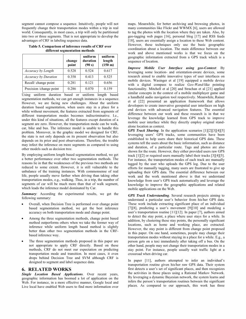
Table 5. Comparison of inference results of CRF over

different segmentation methods

change

point

uniform

duration

(90 s)

uniform

length

(150 m)

Accuracy by Length 0.528 0.524 0.617

Accuracy by Duration 0.358 0.413 0.525

Recall/ change point 0.281 0.121 0.656

Precision /change point 0.286 0.070 0.159

Using uniform duration based or uniform length based

segmentation methods, we can get enough instances in a sequence.

However, we are facing new challenges. About the uniform

duration based segmentation, when users stay in a place for a

while without movement, the features extracted from segments of

different transportation modes becomes indiscriminative. I.e.,

under this kind of situations, all the features except duration of a

segment are zero. However, the transportation mode can be walk,

car, bike and bus. The inference model is unable to handle this

problem. Moreover, in the graphic model we designed for CRF,

the state is not only depends on its present observation but also

depends on its prior and post observations. Therefore, the trouble

may infect the inference on more segments as compared to using

other models such as decision tree.

By employing uniform length based segmentation method, we get

a better performance over other two segmentation methods. The

reasons lie in that the weaknesses of the previous two methods are

reduced to some extent. However, it is still vulnerable to the

unbalance of the training instances. With commonsense of real

life, people usually move farther when driving than taking other

transportation modes, e.g., walking. Thus, in a trip, the number of

segments of car will be much more than that of walk segment,

which leads the inference model dominated by Car.

Summary: According the experimental results, we get the

following summary:

Overall, when Decision Tree is performed over change point

based segmentation method, we get the best inference

accuracy on both transportation mode and change point.

Among the three segmentation methods, change point based

method outperforms others when we take the former way of

inference while uniform length based method is slightly

better than other two segmentation methods in the CRF-

based inference way.

The three segmentation methods proposed in this paper are

not appropriate to apply CRF directly. Based on these

methods, CRF do not meet our expectation on predicting

transportation mode and transition. In most cases, it even

drops behind Decision Tree and SVM although CRF is

designed to segment and label sequence data.

6. RELATED WORKS Single Location Based Applications. Over recent years,

geographic information has boomed a lot of application on the

Web. For instance, in a more effective manner, Google local and

Live local have enabled Web users to find more information over

maps. Meanwhile, for better archiving and browsing photos, in

many communities like Flickr and WWMX [6], users are allowed

to tag the photos with the location where they are taken. Also, by

geo-tagging web pages [16], personal blog [17] and RSS feeds

[18], users are essentially assign a location to these Web content.

However, these techniques only use the basic geographic

coordination about a location. The main difference between our

work and above mentioned works is that we focus on the

geographic information extracted from a GPS track which is a

sequence of location.

Improve Mobile User Interface using geo-Context: By

leveraging some location- and orientation-aware devices, some

research aimed to enable innovative types of user interfaces on

mobile devices. Wasinger et al [19] equipped a mobile device

with a digital compass to realize Geo-Wand-like pointing

functionality. Mitchell et al [20] and Strachan et al [21] applied

similar concepts in the context of a mobile multiplayer game and

a handheld audio navigation tool respectively. Meanwhile, Rainer

et al [22] presented an application framework that allows

developers to create innovative geospatial user interfaces on high

end devices with advanced navigation features. The essential

difference between our work and these research is in that we

leverage the knowledge learned from GPS track to improve

mobile user interface while they directly employ original stand-

alone location as context.

GPS Track Sharing. In the application scenarios [1][2][3][4][5]

leveraging users’ GPS tracks, some communities have been

established to help users share their historical GPS data. These

systems tell the users about the basic information, such as distance

and duration, of a particular route. Tags and photos are also

shown for the route. However, they either provided users raw GPS

track [1][2] or required users manually label their tracks [3][4][5].

For instance, the transportation modes of each track are manually

tagged by the user who uploads the GPS log. Due to the user

efforts for manually tagging, many users are frustrated to give up

uploading their GPS data. The essential difference between our

work and the work mentioned above is that we understand

knowledge from user’s GPS track automatically and leverage the

knowledge to improve the geographic applications and related

mobile applications on the Web.

GPS Track Understanding. Several research projects aiming to

understand a particular user’s behavior from his/her GPS data.

These work include extracting significant place of an individual

[7][8], predicting a user’s movement [9][10] and modeling a

user’s transportation routine [11][12]. In paper [7], authors aimed

to detect the stay point, a place where user stays for a while. In

addition, by clustering these stay points, the personally significant

locations, such as home and working place, are extracted.

However, the stay point is different from change point proposed

in this paper. On one hand, sometimes, people may change their

transportation modes without staying in a place for a while. E.g., a

person gets on a taxi immediately after taking off a bus. On the

other hand, people may not change their transportation modes in a

stay point. For instance, people usually wait traffic light at a

crossroad when driving car.

In paper [11], authors attempted to infer an individual’s

transportation routine given his/her raw GPS data. Their system

first detects a user’s set of significant places, and then recognizes

the activities in those places using a Rational Markov Network.

By leveraging a dynamic Bayesian network, the system learns and

infers the person’s transportation routines between the significant

places. As compared to our approach, this work has three

constraints: 1) It needs the information of road networks, bus

stops and parking lots. 2) It also needs the location of a user’s car,

which implies two GPS receivers are needed. 3) Given above

supplementary information, the model learned from a particular

user’s historical GPS data are customized for the user. I.e., each

user needs a personal model learned from his/her historical GPS

data respectively. Thus, it is not universal and general to be

implemented on the website for public geographic applications.

The main difference between our work and the research

mentioned above is that we mine the knowledge from the GPS

data collected by multi-users while the knowledge can also

contribute to both personal use and public use.

7. CONCLUSIONS In this paper, by using knowledge mined from raw GPS data, we

aim to improve geographic applications on the Web and build

closer connections between locality and mobility. The knowledge

we gained as well as the connections enable more novel

applications and improve user experience in a variety of tasks. An

approach has been proposed to automatically learn transportation

mode from raw GPS data. The inferred transportation mode can

help Web users more deeply understand their own experience

while better sharing other users’ knowledge. It also enables

context-aware computing based on a user’s present transportation

mode and creation of innovative user interface for Web users. The

proposed approach is independent of other information and

devices. Therefore, it is universal to be performed in both mobile

devices and servers.

Our approach consists of three parts: a change point based

segmentation method, an inference model and a post-processing

algorithm based on conditional probability. We evaluated our

approach using the GPS data collected by 45 people over a period

of six months. As compared to uniform duration based and

uniform length based segmentation methods, change point based

method achieved a higher degree of accuracy in predicting

transportation modes. It also obtained better precision in detecting

transitions between different transportation modes. Over the

change point based segmentation method, Decision Tree

outperformed other inference models. However, based on the

three segmentation methods mentioned above, CRF did not

present its advantages in labeling sequence data.

In the future, we will strive for improving the prediction

performance of CRF by designing more reasonable segmentation

methods and more sophisticated graphical model for CRF.

Combing different segmentation methods is also potential work to

do. Meanwhile, we are moving forward to learning more

knowledge from raw GPS and hope to leverage them to improve

geographic applications on the Web.

8. REFERENCES [1] Walk Jog Run. http://www.walkjogrun.net/

[2] Mountain Bike. http://www.mtb-

routes.co.uk/northyorkmoors/default.aspx

[3] SportsDo. http://sportsdo.net/Activity/ActivityBlog.aspx

[4] SlamXR. http://www.msslam.com/slamxr/slamxr.htm

[5] Wikiwalki. http://www.wikiwalki.com

[6] Toyama K., Ron L. and Roseway A.. Geographic location

tags on digital images. In Proceedings of ACM

Multimedia ’03 (New York, 2003), ACM Press: 156-166.

[7] Project lachesis: Parsing and modeling location histories, In

Proceedings of GIScienc’04 (Hariharan Toyama, 2004).

Springer Press.

[8] Ashbrook, D., and Starner, T. Using GPS to learn significant

locations and predict movement across multiple users.

Personal and Ubiquitous Computing 7(5), 275-286.

[9] Krumm J. and Horvitz E. Predestination: Inferring

Destinations from Partial Trajectories. In Proceedings of

UBICOMP’06 (California USA, September 2006), Springer-

Verlag Press: 243-260

[10] Patterson, D. J., Liao and L., Fox, D. Inferring High-Level

Behavior from Low-Level Sensors. In Proceedings of

UBICOMP ’03 (Seattle WA, September 2003), Springer-

Verlag Press: 73-89

[11] Liao L., Patterson D.J., Fox D., and Kautz H. Building

Personal Maps from GPS Data. IJCAI MOO05, 2005

[12] Liao L., Patterson D.J., Fox D., and Kautz H.. Learning and

Inferring Transportation Routines. In Proceedings of the

National Conference on Artificial Intelligence (2004), AAAI

Press: 348-353.

[13] Lafferty, J., McCallum, A., Pereira, F. Conditional random

fields: Probabilistic models for segmenting and labeling

sequence data. In Proceedings of the 18th International Conf.

on Machine Learning (San Francisco CA, 2001). ACM Press:

282–289

[14] Weka. http://www.cs.waikato.ac.nz/ml/weka/

[15] CRF++. http://crfpp.sourceforge.net/#training

[16] Tezuka, T., Kurashima, T., and Tanaka, K. Toward tighter

integration of web search with a geographic information

system. In Proceedings of WWW '06 (Edinburgh Scotland,

May 2006). ACM Press: 277-286

[17] twittervision. http://twittervision.com/

[18] Chen Y. F., Fabbrizio G. D., Gibbon D., Jana R., Jora S.,

Renger B., Wei B. GeoTracker: Geospatial and Temporal

RSS Navigation. In Proceedings of WWW '06 (New

Brunswick Scotland, May 2007). ACM Press: 41-50.

[19] Wasinger, R., Stahl, C., Krüger, A. M3I in a Pedestrian

Navigation & Exploration System. In Proceedings of

MobileHCI '03, (Udine Italy, September 2003). Springer-

Verlag Press: 481-485

[20] Mitchell, K., McCaffery, D., Metaxas, G., Finney, J., Schmid,

S., Scott, A. Six in the City: Introducing Real Tournament –

A Mobile Context-Aware Multiplayer Game. In Proceedings

of the 2nd Workshop on Network and System Support for

Games (California USA, May 2003). ACM Press: 91-100.

[21] Strachan, S., Eslambolchilar, P., Murray-Smith, R. gpsTunes

-Controlling Navigation via Audio Feedback. In Proceedings

of MobileHCI '05, (Salzburg Austria, September 2005).

ACM Press: 275-278.

[22] Simon R., Fröhlich P.. A Mobile Application Framework for

the Geospatial Web. In Proceedings of WWW '07 (Banff

Canada, May 2007). ACM Press: 381-390.