Learning Topology and Dynamics of LargeRecurrent Neural Networks

Yiyuan She, Yuejia He, and Dapeng Wu, Fellow, IEEE

Abstract—Large-scale recurrent networks have drawn increas-ing attention recently because of their capabilities in modeling alarge variety of real-world phenomena and physical mechanisms.This paper studies how to identify all authentic connections andestimate system parameters of a recurrent network, given asequence of node observations. This task becomes extremely chal-lenging in modern network applications, because the availableobservations are usually very noisy and limited, and the associ-ated dynamical system is strongly nonlinear. By formulating theproblem as multivariate sparse sigmoidal regression, we developsimple-to-implement network learning algorithms, with rigorousconvergence guarantee in theory, for a variety of sparsity-promoting penalty forms. A quantile variant of progressiverecurrent network screening is proposed for efficient computationand allows for direct cardinality control of network topology inestimation. Moreover, we investigate recurrent network stabilityconditions in Lyapunov’s sense, and integrate such stabilityconstraints into sparse network learning. Experiments showexcellent performance of the proposed algorithms in networktopology identification and forecasting.

Index Terms—Recurrent networks, topology learning, shrink-age estimation, variable selection, dynamical systems, Lyapunovstability.

I. INTRODUCTION

There has been an increasing interest in identifying networkdynamics and topologies in the emerging scientific disciplineof network science. In a dynamical network, the evolution ofa node is controlled not only by itself, but also by other nodes.For example, in gene regulatory networks [1], the expressionlevels of genes influence each other, following some dynamicrules, such that the genes are connected together to form adynamical system. If the topology and evolution rules of thenetwork are known, we can analyze the regulation betweengenes or detect unusual behaviors to help diagnose and curegenetic diseases. Similarly, the modeling and estimation of dy-namical networks are of great importance in various domainsincluding stock market, brain network and social network[2, 3, 4]. To accurately identify the topology and dynamicsunderlying those networks, scientists are devoted to developingappropriate mathematical models and corresponding estima-tion methods.

In the literature, linear dynamical models are commonly

Copyright (c) 2014 IEEE. Personal use of this material is permitted.However, permission to use this material for any other purposes must beobtained from the IEEE by sending a request to pubs-permissions@ieee.org.

Yiyuan She is with Department of Statistics, Florida State University,Tallahassee, FL 32306. Yuejia He and Dapeng Wu are with Departmentof Electrical and Computer Engineering, University of Florida, Gainesville,FL 32611. Correspondence author: Prof. Dapeng Wu, wu@ece.ufl.edu,http://www.wu.ece.ufl.edu. This work was supported in part by NSF grantsCCF-1117012, CCF-1116447 and DMS-1352259.

used. For example, the human brain connectivity network [5]can be characterized by a set of linear differential equations,where the rate of change of activation/observation of anynode is a weighted sum of the activations/observations of itsneighbors: dxi/dt =

∑j =i αijxj − dixi, 1 ≤ i ≤ n. Here

αij provide the connection weights and di is the decay rate.Nevertheless, a lot of complex dynamical networks clearlydemonstrate nonlinear relationships between the nodes. Forinstance, the strength of influence is unbounded in the previoussimple linear combination, but the so-called “saturation”effect widely exists in physical/biological systems (neurons,genes, and stocks)—the external influence on a node, no matterhow strong the total input activation is, cannot go beyonda certain threshold. To capture the mechanism, nonlinearitymust be introduced into the network system: dxi/dt =liπ(

∑j =i αijxj+ui)−dixi+ci, where π denotes a nonlinear

activation function typically taken to be the sigmoidal functionπ(θ) = 1/(1 + e−θ). It has a proper shape to resemble manyreal-world mechanisms and behaviors.

The model description is associated with a continuous-timerecurrent neural network. The existing feedback loops allowthe network to exhibit interesting dynamic temporal behaviorsto capture many kinds of relationships. It is also biologicallyrealistic in say modeling the effect of an input spike train.Recurrent networks have been successfully applied to a widerange of problems in bioinformatics, financial market forecast,electric circuits, computer vision, and robotics; see, e.g., [6,7, 8, 9, 10] among many others.

In practical applications, it is often necessary to includenoise contamination: dxi = (liπ(

∑j =i αijxj + ui)− dixi +

ci) dt + σ dBt, 1 ≤ i ≤ n, where Bt stands for an n-dimensional Brownian motion. Among the very many un-known parameters, αij might be the most important: the zero-nonzero pattern of αij indicates if there exists a (direct) con-nection from node j to node i. Collecting all such connectionsresults in a directed graph to describe the node interactionstructure.

A fundamental question naturally arises: Given a sequenceof node observations (possibly at very few time points), canone identify all existing connections and estimate all systemparameters of a recurrent network?

This task becomes extremely challenging in modern bignetwork applications, because the available observations areusually very noisy and only available at a relatively smallnumber of time points (say T ), due to budget or equipmentlimitations. One frequently faces applications with n2 muchlarger than T . In addition, in this continuous time setting, noanalytical formula of the likelihood exists for the stochastic

2

model, which increases the estimation difficulty even in largesamples [11]. Instead of considering multi-step ad-hoc pro-cedures, this paper aims at learning the network system as awhole. Multivariate statistical techniques will be developed foridentifying complete topology and recovering all dynamicalparameters. To the best of our knowledge, automatic topologyand dynamics learning in large-scale recurrent networks hasnot been studied before.

In this work, we are interested in networks that are sparse intopology. First, many real-world complex dynamical networksindeed have sparse or approximately sparse structures. Forexample, in regulatory networks, a gene is only regulatedby a handful of others [12]. Second, when the number ofnodes is large or very large compared with the number ofobservations, the sparsity assumption reduces the number ofmodel parameters so that the system is estimable. Third, froma philosophical point of view, a sparse network modeling isconsistent with the principle of Occam’s razor.

Not surprisingly, there is a surge of interest of using com-pressive sensing techniques for parsimonious network topol-ogy learning and dynamics prediction. However, relying onsparsity alone seems to have only limited power in addressingthe difficulties of large-scale network learning from big data.To add more prior knowledge and to further reduce the numberof effective unknowns, we propose to study how to incorporatestructural properties of the network system into learning andestimation, in addition to sparsity. In fact, real-life networks ofinterest usually demonstrate asymptotic stability. This is oneof the main reasons why practitioners only perform limitednumber of measurements of the system, which again providesa type of parsimony or shrinkage in network learning.

In this paper we develop sparse sigmoidal network learningalgorithms, with rigorous convergence guarantee in theory, fora variety of sparsity-promoting penalty forms. A quantile vari-ant, the progressive recurrent network screening, is proposedfor efficient computation and allows for direct cardinalitycontrol of network topology in estimation. Moreover, we in-vestigate recurrent network stability conditions in Lyapunov’ssense, and incorporate such stability constraints into sparsenetwork learning. The remaining of this paper is organized asfollows. Section II introduces the sigmoidal recurrent networkmodel, and formulates a multivariate regularized problembased on the discrete-time approximate likelihood. Section IIIproposes a class of sparse network learning algorithms basedon the study of sparse sigmoidal regressions. A novel andefficient recurrent network screening (RNS) with theoreticalguarantee of convergence is advocated for topology identifica-tion in ultra-high dimensions. Section IV investigates asymp-totic stability conditions in recurrent systems, resulting in astable-sparse sigmoidal (S3) network learning. In Section V,synthetic data experiments and real applications are given. Allproof details are left to the Appendices.

II. MODEL FORMULATION

To describe the evolving state of a continuous-time recurrentneural network, one usually defines an associated dynamicalsystem. Ideally, without any randomness, the network behavior

can be specified by a set of ordinary differential equations:

dxidt

= liπ(∑j =i

αijxj + ui)− dixi + ci, i = 1, · · · , n,

(1)

where xi, short for xi(t), denotes the dynamic process of nodei. Throughout the paper, π is the sigmoidal activation function

π(θ) =1

1 + e−θ, (2)

which is most frequently used in recurrent networks. Thisfunction is smooth and strictly increasing. It has a propershape to resemble many real-world mechanisms and behaviors.Due to noise contamination, a stochastic differential equationmodel is more realistic

dxi = (liπ(∑j =i

αijxj + ui)− dixi + ci) dt+ σ dBt, (3)

where Bt is a standard Brownian motion and reflects thestochastic nature of the system. Typically li > 0, di > 0, andin some applications αii = 0 (no self-regulation) is required.

In the sigmoidal recurrent network model, the coefficientsαij characterize the between-node interactions. In particular,αij = 0 indicates that node j does not directly influencenode i; otherwise, node j regulates node i, and is referredto as a regulator of node i in gene regulatory networks.Such a regulation relationship can be either excitatory (if αij

is positive) or inhibitory (if αij is negative). In this way,A = [αij ] is associated with a directed graph that capturesthe Granger causal relationships between all nodes [13], andthe topology of the recurrent network is revealed by thezero-nonzero pattern of the matrix. Therefore, to identify allsignificant regulation links, it is of great interest to estimateA, given a sequence of node observations (snapshots of thenetwork).

Denote the system state at time t by x(t) =[x1(t) · · ·xn(t)]T or xt (or simply x when there is noambiguity.) Define l = [l1, · · · ln]T, u = [u1, · · · , un]T,c = [c1, · · · , cn]T, D = diag{di}, L = diag{li}, andA = [αij ] = [α1 · · ·αn]

T ∈ Rn×n. Then (3) can berepresented in a multivariate form

dxt = (Lπ(Ax+ u)−Dx+ c) dt+ σ dBt, (4)

where Bt is an n-dimensional standard Brownian motion.While this model is specified in continuous time, in practice,the observations are always collected at discrete time points.Estimating the parameters of an SDE model from few discreteobservations is very challenging. There rarely exists an analyt-ical expression of the exact likelihood. A common treatmentis to discretize (4) and use an approximate likelihood instead.We use the Euler discretization scheme (see, e.g., [14]):

∆x = (Lπ(Ax+ u)−Dx+ c)∆t+ σ∆Bt.

Suppose the system (4) is observed at T + 1 time pointst1, · · · , tT+1. Let xs = [x1(ts), · · · , xn(ts)]T ∈ Rn bethe observed values of all n nodes at ts. Define ∆xs =(xs+1 − xs) and ∆ts = (ts+1 − ts), 1 ≤ s ≤ T . Because∆Bt ∼ N (0,∆tI), the negative conditional log-likelihood

3

for the discretized model is given by

ℓ(x1, · · · ,xT+1|x1) = − logP (∆x1, · · · ,∆xT |x1)

=− logP (∆x1|x1) · · ·P (∆xT |xT )

=

T∑s=1

∥∆xs/∆ts − (Lπ(Axs + u)−Dxs + c)∥22∆ts/(2σ2)

+ C(σ2) =: f(A,u, l,d, c)/σ2 + C(σ2).

C(σ2 is a function that depends on σ2 only. The fitting crite-rion f is separable in α1, . . . ,αn. To see this, let xi,s = xi(ts)and ∆xi,s = xi(ts+1)− xi(ts). Then, it is easy to verify that

f(A,u, l,d, c)

=1

2

n∑i=1

T∑s=1

(∆xi,s∆ts

− (liπ(αTi xs + ui)− dixi,s + ci)

)2

∆ts.

(5)

Conventionally, the unknown parameters can then be estimatedby minimizing f . In modern applications, however, the numberof available observations (T ) is often much smaller thanthe number of variables to be estimated (n2 + 4n), due to,for example, equipment/budget limitations. Classical MLEmethods do not apply well in this high-dimensional setting.

Fortunately, the networks of interest in reality often possesstopology sparsity. For example, a stock price may not bedirectly influenced by all the other stocks in the stock market.A parsimonious network with only significant regulation linksis much more interpretable. Statistically speaking, the sparsityin A suggests the necessity of shrinkage estimation [15]which can be done by adding penalties and/or constraints tothe loss function. The general penalized maximum likelihoodproblem is

minA,u,l,d,c

f(A,u, l,d, c) +∑i,j

P (αij ;λji) (6)

where P is a penalty promoting sparsity and λji are regular-ization parameters. Among the very many possible choices ofP , the ℓ1 penalty is perhaps the popular nowadays to enforcesparsity:

P (t;λ) = λ|t|. (7)

It provides a convex relaxation of the ℓ0 penalty

P (t;λ) =λ2

21t =0. (8)

Taking both topology identification and dynamics predictioninto consideration, we are particularly interested in the ℓ0+ℓ2penalty [16]

P (t;λ, η) =1

2

λ2

1 + η1t =0 +

η

2t2, (9)

where the ℓ2 penalty or Tikhonov regularization can effectivelydeal with large noise and collinearity [17, 18] to enhanceestimation accuracy.

The shrinkage estimation problem (6) is however nontrivial.The loss f is nonconvex, π is nonlinear, and the penaltyP may be nonconvex or even discrete, let alone the high-dimensionality challenge. Indeed, in many practical networks,

the available observations are usually quite limited and noisy.Effective and efficient learning algorithms are in great need tomeet the modern big data challenge.

III. SPARSE SIGMOIDAL REGRESSION FOR RECURRENTNETWORK LEARNING

A. Univariate-response sigmoidal regression

As analyzed previously, to solve (6), it is sufficient to studya univariate-response learning problem

min(β,l,γ)

1

2

T∑s=1

ws

(ys − lπ(xT

sβ)− zTs γ)2

+n∑

k=1

P (βk, λk)

, F (β, l,γ)(10)

where xs, zs, ys, ws are given, and l,γ,β are unknown withβ desired to be sparse. (10) is the recurrent network learningproblem for node i when we set xs = [1,xs]

T, ys =∆xi,s/∆ts, zs = [1, xi,s]

T, and ws = ∆ts (1 ≤ s ≤ T )(note that the intercept β1 is usually subject to no penaliza-tion corresponding to λ1 = 0). For notational ease, defineX = [x1, · · · , xT ]

T, y = [y1, · · · , yT ]T, Z = [z1, · · · , zT ]T,

λ = [λk] ∈ Rn, and W = diag{w} = diag{w1, · · · , ws} (tobe used in this subsection only, unless otherwise specified).

We propose a simple-to-implement and efficient algorithmto solve the general optimization problem in the form of (10).First define two useful auxiliary functions

ξ(θ, y) = π(θ)(1− π(θ))(π(θ)− y), (11)

k0(y,w) = max1≤s≤T

ws

16

(1 +

(1− 2ys)2

2

). (12)

The vector versions of π and ξ are defined compo-nentwise: π(θ) = [π(θ1), · · · , π(θT )]T and ξ(θ,y) =[ξ(θ1, y1), · · · , ξ(θT , yT )]T, and the matrix versions are de-fined similarly. A prototype algorithm is described as follows,starting with an initial estimate β(0), a thresholding rule Θ(an odd, shrinking and nondecreasing function, cf. [19]), andj = 0.

repeat0) j ← j + 11) µ(j) ← π(Xβ(j−1))2) Fit a weighted least-squares model

minl,γ∥W 1/2(y − [µ(j) Z][l γT]T)∥22, (13)

with the corresponding solution denoted by (l(j),γ(j)).3) Construct y(j) ← (y−Zγ(j))/l(j), w(j) ← (l(j))2w,W

(j)= diag{w(j)}. Let K(j) be any constant no less

than k0(y(j), w(j))∥X∥22, where ∥ · ∥2 is the spectral

norm.4) Update β via thresholding:

β(j) = Θ(β(j−1)− 1

K(j)X

TW

(j)ξ(Xβ(j−1), y(j));λ(j)),

(14)where λ(j) = [λ

(j)k ]n×1 is a scaled version of λ satisfying

P (t;λk)/K(j) = P (t;λ

(j)k ) for any t ∈ R , 1 ≤ k ≤ n.

until convergence

4

Before proceeding, we give some examples of Θ and λ(j).The specific form of the thresholding function Θ in (14) isrelated to the penalty P through the following formula [16]:

P (t;λ)− P (0;λ)

=

∫ |t|

0

(sup{s : Θ(s;λ) ≤ u} − u) du+ q(t;λ)(15)

with q(·;λ) nonnegative and q(Θ(s;λ)) = 0 for all s. The reg-ularization parameter(s) are rescaled at each iteration accord-ing to the form of P . Examples include: (i) the ℓ1 penalty (7),and its associated soft-thresholding ΘS(t;λ) = sgn(t)(|t| −λ)1|t|>λ, in which case P (t;λ)/K(j) = P (t;λ(j)), ∀t im-plies λ(j) = λ/K(j), (ii) the ℓ0 penalty (8) and the hard-thresholding ΘH(t) = t1|t|>λ, which determines λ(j) =

λ/√K(j), and (iii) the ℓ0 + ℓ2 penalty (9) and its associated

hard-ridge thresholding ΘHR(t;λ, η) = t1+η1|t|>λ, where

λ(j) = λK(j)

√(η +K(j))/(η + 1), η(j) = η/K(j). The ℓp

(0 < p < 1) penalties, the elastic net penalty, and others[16] are also instances of this framework.

Theorem 1. Given the objective function in (10), supposeΘ and P satisfy (15) for some nonnegative q(t;λ) withq(Θ(t;λ)) = 0 for all t and λ. Then given any ini-tial point β(0), with probability 1 the sequence of iterates(β(j), l(j),γ(j)) generated by the prototype algorithm satisfies

F (β(j−1), l(j−1),γ(j−1)) ≥ F (β(j), l(j),γ(j)). (16)

See Appendix A for the proof.Normalization is usually necessary to make all predictors

equally span in the space before penalizing their coefficientsusing a single regularization parameter λ. We can center andscale all predictor columns but the intercept before calling thealgorithm. Alternatively, it is sometimes more convenient tospecify λk componentwise—e.g., in the ℓ1 penalty

∑λk|βk|

set λk = λ · ∥X[:, k]∥2 for non-intercept coefficients.

B. Cardinality constrained sigmoidal network learning

In the recurrent network setting, one can directly applythe prototype algorithm in Section III-A to solve (6), byupdating the columns in B one at a time. On the otherhand, a multivariate update form is usually more efficientand convenient in implementation. Moreover, it facilitatesintegrating stability into network learning (cf. Section IV).

To formulate the loss in a multivariate form, we introduce

Y = [yi,s] = [∆xi,s/∆ts] ∈ RT×n,

X = [x1, · · · ,xT ]T ∈ RT×n,

B = AT = [α1, · · · ,αn] ∈ Rn×n,

W = diag{w} = diag{∆t1, · · · ,∆tT }.

Then f in (5) can be rewritten as

f(B,u, l,d, c)

=1

2∥W 1/2

{Y − [π(XB + 1uT)L−XD + 1cT]

}∥2F ,

(17)

with ∥ · ∥F denoting the Frobenius norm, and the objec-tive function to minimize becomes ∥W 1/2{Y − [π(XB +

1uT)L−XD + 1cT]}∥2F + P (B,Λ).

One of the main issues is to choose a proper penalty form forsparse network learning. Popular sparsity-promoting penaltiesinclude ℓ1, SCAD, ℓ0, among others. The ℓ0 penalty (8) isideal in pursuing a parsimonious solution. However, the matterof parameter tuning cannot be ignored. Most tuning strategies(such as K-fold cross-validation) require computing a solutionpath for a grid of values of λ, which is quite time-consuming inlarge network estimation. Rather than applying the ℓ0 penalty,we propose an ℓ0 constrained sparse network learning

∥B∥0 ≤ m, (18)

where ∥ · ∥0 denotes the number of nonzero componentsin a matrix. In contrast to the penalty parameter λ in (8),m is more meaningful and customizable. One can directlyspecify its value based on prior knowledge or availabilityof computational resources to have control of the networkconnection cardinality. To account for collinearity and largenoise contamination, we add a further ℓ2 penalty in B,resulting in a new ‘ℓ0 + ℓ2’ regularized criterion

minB,L,D,u,c

1

2∥W 1/2{Y − [π(XB + 1uT)L−XD + 1cT]}∥2F

+η

2∥B∥2F =: F0, s.t. ∥B∥0 ≤ m.

(19)Not only is the cardinality bound m convenient to set, becauseof the sparsity assumption, but the ℓ2 shrinkage parameterη is easy to tune. Indeed, η is usually not a very sensitiveparameter and does not require a large grid of candidate values.Many researchers simply fix it at a small value (say, 1e − 3)which can effectively reduce the prediction error (e.g., [18]).Similarly, to handle the possible collinearity between π and 1,we recommend adding mild ridge penalties ηl

2 ∥l∥22 +

ηc

2 ∥c∥22

in (19) (say, ηl = 1e− 4 and ηc = 1e− 2).The constrained optimization of (19) does not apparently

fall into the penalized framework proposed in Section III-A.However, we can adapt the technique to handle it through aquantile thresholding operator (as a variant of the hard-ridgethresholding (9)). The detailed recurrent network screening(RNS) algorithm is described as follows, where for notationalsimplicity X := [1 X], B := [u BT]T, and we denote byA[I, J ] the submatrix of A consisting of the rows and columnsindexed by I and J , respectively.

Theorem 2. Given any initial point B(0)

, Algorithm 1 con-verges in the sense that with probability 1, the function valuedecreasing property holds:

F0(B(j−1),L(j−1),D(j−1),u(j−1), c(j−1))

≥ F0(B(j),L(j),D(j),u(j), c(j)),

and all B(j) satisfy ∥B(j)∥0 ≤ m, ∀j ≥ 1.

See Appendix B for the proof.Step 2 can be achieved by solving n weighted least squares.

Or, one can re-formulate it as a single-response problem toobtain the solution (l(j),d(j), c(j)) in one step. The latterway is usually more efficient. When there are ridge penaltiesimposed on l and c, the computation is similar.

5

Algorithm 1 Recurrent Network Screening (RNS)

given B(0)

(initial estimate), m (cardinality bound), η (ℓ2shrinkage parameter).j ← 0repeat

0) j ← j + 1

1) µ(j) ← π(XB(j−1)

)2) Update L = diag{l},D = diag{d}, and c by fittinga weighted vector least-squares model:

minL,D,c

∥W 1/2(Y − [µ(j)L−XD + 1cT])∥2F , (20)

with the solution denoted by L(j) = diag{l(j)} =

diag{l(j)1 , · · · , l(j)n }, D(j) = diag{d(j)1 , · · · , d(j)n }, andc(j). (This amounts to solving n separate weighted leastsquares problems.)3) Construct Y ← (Y + XD(j) − 1(c(j))T)(L(j))−,W ← w · (l(j) ◦ l(j))T, where − denotes the Moore-Penrose pseudoinverse and ◦ is the Hadamard product.Let K(j)

i be any constant no less than k0(Y [:, i], W [:

, i]])∥X∥22, and K(j) ← diag{K(j)1 , · · · ,K(j)

n }.4) Update B and u:4.1) Ξ← B

(j−1)−XT{W ◦ξ(XB

(j−1), Y )}(K(j))−,

u(j) ← (Ξ[1, :])T, Ξ ← Ξ[2 : end, :] (the submatrix ofΞ without the first row), η(j) = η · (11T)(K(j))−.4.2) Perform the hard-ridge thresholding B(j) ←ΘHR

(Ξ; ζ(Ξ),η(j)

)(cf. Section III-A for the definition

of ΘHR) with an adaptive threshold matrix ζ(Ξ). Theentries of ζ(Ξ) are all set to the medium of the mth andthe (m + 1)th largest components of vec(|Ξ|). See (21)for other variants when certain links must be maintainedor forbidden.4.3) B

(j) ← [u(j) (B(j))T]T

until the decrease in function value is smalldeliver B = B(j), u = u(j), L = L(j), D = D(j),c = c(j).

In certain applications self-regulations are not allowed. Thenζ(Ξ) should be the medium of the mth and the (m + 1)thlargest elements of |Ξ − Ξ ◦ I| (Ξ in absolute value afterexcluding its diagonal entries).1 Other prohibited links canbe similarly treated in determining the dynamic threshold.In general, given T the index set of the links that must bemaintained and F the index set of the links that are forbidden,the threshold is constructed as follows

Ξ[i]← 0, ∀i ∈ F

ζ[i]←

{0, if i ∈ T|Ξ[T c]|(m+1) , otherwise,

(21)

where |Ξ[T c]|(m+1) is the (m + 1)th largest element (inabsolution value) in Ξ[T c] (all entries of Ξ except thoseindexed by T ). It is easy to show that the convergence resultstill holds based on the argument in Appendix B.

1Throughout the paper |A| is the absolute value of the elements of A. Thatis, for A = [aij ], |A| = [|aij |].

In implementation, we advocate reducing the network car-dinality in a progressive manner to lessen greediness: at thejth step, m is replaced by m(j), where {m(j)} is a monotonesequence of integers decreasing from n(n− 1) (assuming noself-regulation) to m. Empirical study shows that the sigmoidaldecay cooling schedule m(j) =

⌈2n(n − 1)/(1 + eαj)

⌉with

α = 0.01, works well.RNS involves no costly operations at each iteration, and is

simple to implement. It runs efficiently for large networks.The RNS estimate can be directly used for analyzing thenetwork topology. One can also use it for screening (in whichcase a relatively large value of m is specified), followed bya fine network learning algorithm restricted on the screenedconnections. In either case RNS substantially reduces thesearch space of candidate links.

IV. STABLE-SPARSE SIGMOIDAL NETWORK LEARNING

For a general dynamical system possibly nonlinear, stabilityis one of the most fundamental issues [20, 21]. If a system’sequilibrium point is asymptotically stable, then the perturbedsystem must approach the equilibrium point as t increases.Moreover, one of the main reasons many real network applica-tions only have limited number of observations measured afterperturbation is that the associated dynamical systems stabilizefast (e.g., exponentially fast). This offers another importanttype of parsimony/shrinkage in network parameter estimation.

To design a new type of regularization, we first investi-gate stability conditions of sigmoidal recurrent networks inLyapunov’s sense [22, 23]. Then, we develop a stable sparsesigmoidal (S3) network learning approach.

A. Conditions for asymptotic stability

Recall the multivariate representation of (1)

dx

dt= Lπ(Ax+ u)−Dx+ c. (22)

Because A is sparse and typically singular and the degradationrates di are not necessarily identical, in general (22) can not betreated as an instance of the Cohen-Grossberg neural networks[24]. We must first derive its own stability conditions to beconsidered in network estimation.

Hereinafter, A ≽ A′ and A ≻ A′ stand for the posi-tive semi-definiteness and positive definiteness of A − A′,respectively, and the set of eigenvalues of A is spec(A). Ourconditions are stated below:

D ≻ 0, (A1)L ≽ 0, (A2)

Re(λ) < 0 for any λ ∈ Spec(LA− 4D), (A3a)

LA/2 +ATL/2 ≺ 4D, (A3b)

Theorem 3. Suppose (A1) & (A2) hold. Then (A3a) guar-antees the network defined by (22) has a unique equilibriumpoint x∗ and is globally exponentially stable in the sense that∥x(t)−x∗∥22 ≤ e−εt∥x(0)−x∗∥22 for any solution x(t). Thesame conclusion holds if (A3a) is replaced by (A3b).

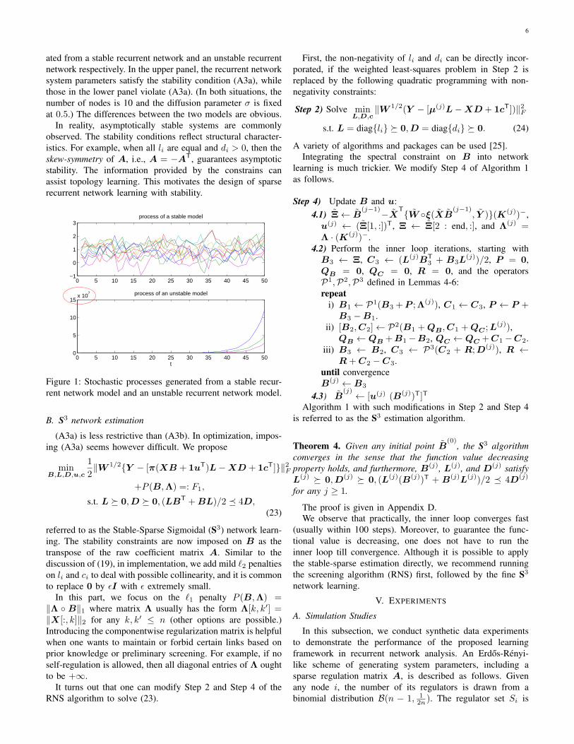
See Appendix C for the detailed proof.Figure 1 shows an example of stochastic processes gener-

6

ated from a stable recurrent network and an unstable recurrentnetwork respectively. In the upper panel, the recurrent networksystem parameters satisfy the stability condition (A3a), whilethose in the lower panel violate (A3a). (In both situations, thenumber of nodes is 10 and the diffusion parameter σ is fixedat 0.5.) The differences between the two models are obvious.

In reality, asymptotically stable systems are commonlyobserved. The stability conditions reflect structural character-istics. For example, when all li are equal and di > 0, then theskew-symmetry of A, i.e., A = −AT, guarantees asymptoticstability. The information provided by the constrains canassist topology learning. This motivates the design of sparserecurrent network learning with stability.

0 5 10 15 20 25 30 35 40 45 50−1

0

1

2

3process of a stable model

0 5 10 15 20 25 30 35 40 45 500

5

10

15x 10

7 process of an unstable model

t

Figure 1: Stochastic processes generated from a stable recur-rent network model and an unstable recurrent network model.

B. S3 network estimation

(A3a) is less restrictive than (A3b). In optimization, impos-ing (A3a) seems however difficult. We propose

minB,L,D,u,c

1

2∥W 1/2{Y − [π(XB + 1uT)L−XD + 1cT]}∥2F

+P (B,Λ) =: F1,

s.t. L ≽ 0,D ≽ 0, (LBT +BL)/2 ≼ 4D,(23)

referred to as the Stable-Sparse Sigmoidal (S3) network learn-ing. The stability constraints are now imposed on B as thetranspose of the raw coefficient matrix A. Similar to thediscussion of (19), in implementation, we add mild ℓ2 penaltieson li and ci to deal with possible collinearity, and it is commonto replace 0 by ϵI with ϵ extremely small.

In this part, we focus on the ℓ1 penalty P (B,Λ) =∥Λ ◦ B∥1 where matrix Λ usually has the form Λ[k, k′] =∥X[:, k]∥2 for any k, k′ ≤ n (other options are possible.)Introducing the componentwise regularization matrix is helpfulwhen one wants to maintain or forbid certain links based onprior knowledge or preliminary screening. For example, if noself-regulation is allowed, then all diagonal entries of Λ oughtto be +∞.

It turns out that one can modify Step 2 and Step 4 of theRNS algorithm to solve (23).

First, the non-negativity of li and di can be directly incor-porated, if the weighted least-squares problem in Step 2 isreplaced by the following quadratic programming with non-negativity constraints:

Step 2) Solve minL,D,c

∥W 1/2(Y − [µ(j)L−XD + 1cT])∥2F

s.t. L = diag{li} ≽ 0,D = diag{di} ≽ 0. (24)

A variety of algorithms and packages can be used [25].Integrating the spectral constraint on B into network

learning is much trickier. We modify Step 4 of Algorithm 1as follows.

Step 4) Update B and u:4.1) Ξ← B

(j−1)−XT{W ◦ξ(XB(j−1)

, Y )}(K(j))−,u(j) ← (Ξ[1, :])T, Ξ ← Ξ[2 : end, :], and Λ(j) =Λ · (K(j))−.

4.2) Perform the inner loop iterations, starting withB3 ← Ξ, C3 ← (L(j)BT

3 + B3L(j))/2, P = 0,

QB = 0, QC = 0, R = 0, and the operatorsP1,P2,P3 defined in Lemmas 4-6:repeat

i) B1 ← P1(B3 +P ;Λ(j)), C1 ← C3, P ← P +B3 −B1.

ii) [B2,C2]← P2(B1 +QB,C1 +QC ;L(j)),QB ← QB +B1−B2, QC ← QC +C1−C2.

iii) B3 ← B2, C3 ← P3(C2 + R;D(j)), R ←R+C2 −C3.

until convergenceB(j) ← B3

4.3) B(j) ← [u(j) (B(j))T]T

Algorithm 1 with such modifications in Step 2 and Step 4is referred to as the S3 estimation algorithm.

Theorem 4. Given any initial point B(0)

, the S3 algorithmconverges in the sense that the function value decreasingproperty holds, and furthermore, B(j), L(j), and D(j) satisfyL(j) ≽ 0,D(j) ≽ 0, (L(j)(B(j))T + B(j)L(j))/2 ≼ 4D(j)

for any j ≥ 1.

The proof is given in Appendix D.We observe that practically, the inner loop converges fast

(usually within 100 steps). Moreover, to guarantee the func-tional value is decreasing, one does not have to run theinner loop till convergence. Although it is possible to applythe stable-sparse estimation directly, we recommend runningthe screening algorithm (RNS) first, followed by the fine S3

network learning.

V. EXPERIMENTS

A. Simulation Studies

In this subsection, we conduct synthetic data experimentsto demonstrate the performance of the proposed learningframework in recurrent network analysis. An Erdos-Renyi-like scheme of generating system parameters, including asparse regulation matrix A, is described as follows. Givenany node i, the number of its regulators is drawn from abinomial distribution B(n − 1, 1

2n ). The regulator set Si is

7

chosen randomly from the rest (n − 1) nodes (excludingnode i itself). If j /∈ Si, aij = 0. Otherwise, aij follows amixture of two Gaussians N (1.5, 0.12) ad N (−1.5, 0.12) withprobability 1/2 for each. Then draw random l, u, c from Gaus-sian distributions (independently) li ∼ N (1.5, 0.12), ui ∼N (0, 0.12), ci ∼ N (0, 0.12). Finally d is generated so thatthe system satisfies the stability condition (A3a).

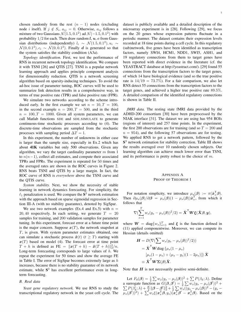
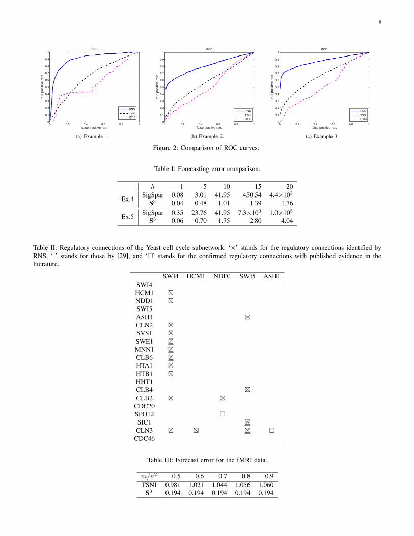
Topology identification. First, we test the performance ofRNS in recurrent network topology identification. We compareit with TSNI [26] and QTIS [27]. TSNI is a popular networklearning approach and applies principle component analysisfor dimensionality reduction. QTIS is a network screeningalgorithm based on sparsity-inducing techniques. To avoid thead-hoc issue of parameter tuning, ROC curves will be used tosummarize link detection results in a comprehensive way, interms of true positive rate (TPR) and false positive rate (FPR).

We simulate two networks according to the scheme intro-duced early. In the first example we set n = 10, T = 100,in the second example n = 200, T = 500, and in the thirdn = 100, T = 1000. Given all system parameters, we cancall Matlab functions SDE and SDE.SIMULATE to generatecontinuous-time stochastic processes according to (4). Thediscrete-time observations are sampled from the stochasticprocesses with sampling period ∆T = 1.

In this experiment, the number of unknowns in either caseis larger than the sample size, especially in Ex.2 which hasabout 41K variables but only 500 observations. Given anyalgorithm, we vary the target cardinality parameter m from 1to n(n−1), collect all estimates, and compute their associatedTPRs and FPRs. The experiment is repeated for 50 times andthe averaged rates are shown in the ROC curves in Figure 2.RNS beats TSNI and QTIS by a large margin. In fact, theROC curve of RNS is everywhere above the TSNI curve andthe QTIS curve.

System stability. Next, we show the necessity of stablelearning in network dynamics forecasting. For simplicity, theℓ1 penalization is used. We compare the S3 network estimationwith the approach based on sparse sigmoidal regression in Sec-tion III-A (with no stability guarantee), denoted by SigSpar.

We use two network examples (Ex.4 and Ex.5) with n =20, 40 respectively. In each setting, we generate T = 20samples for training, and 200 validation samples for parametertuning. In this experiment, forecast error at a future time pointis the major concern. Suppose x(T ), the network snapshot atT , is given. With system parameter estimates obtained, onecan simulate a stochastic process x(t) (t ≥ T ) starting withx(T ) based on model (4). The forecast error at time pointT + h is defined as FE = ∥x(T + h) − x(T + h)∥22/n.Long-term forecasting corresponds to large values of h. Werepeat the experiment for 50 times and show the average FEin Table I. The error of SigSpar becomes extremely large as hincreases, because there is no stability guarantee of its networkestimate, while S3 has excellent performance even in long-term forecasting.

B. Real data

Yeast gene regulatory network. We use RNS to study thetranscriptional regulatory network in the yeast cell cycle. The

dataset is publicly available and a detailed description of themicroarray experiment is in [28]. Following [29], we focuson the 20 genes whose expression patterns fluctuate in aperiodic manner. The dataset contains their expression levelsrecorded at 18 time points during a cell cycle. In this regulatory(sub)network, five genes have been identified as transcriptionfactors, namely SWI4, HCM1, NDD1, SWI5, ASH1, and19 regulatory connections from them to target genes havebeen reported with direct evidence in the literature (cf. theYEASTRACT database at http://yeastract.com/). [29] found 55connections from the transcription factors to the target genes,of which 14 have biological evidence (and so the true positiverate is 14/19 = 73.7%). For a fair comparison, we also letRNS detect 55 connections from the transcription factors to thetarget genes, and achieved a higher true positive rate 89.5%.A detailed comparison of the identified regulatory connectionsis shown in Table II.

fMRI data. The resting state fMRI data provided by theADHD-200 consortium [30] have been preprocessed by theNIAK interface [31]. The dataset we are using has 954 ROIs(regions of interest) and 257 time points. In the experiment,the first 200 observations are for training (and so T = 200 andn = 954), and the following 57 observations are for testing.We applied RNS to get a network pattern, followed by theS3 network estimation for stability correction. Table III showsthe results averaged over 10 randomly chosen subjects. Ourlearning algorithm can achieve much lower error than TSNI,and its performance is pretty robust to the choice of m.

APPENDIX APROOF OF THEOREM 1

For notation simplicity, we introduce µs(β) := π(xTsβ).

Then ∂µs(β)/∂β = µs(β)(1 − µs(β))xTs , from which it

follows that

∇(T∑

s=1

ws(ys − µs(β))2/2) = X

TWξ(Xβ,y),

where W = diag{ws}Ts=1 and ξ is the function defined in(11) applied componentwise. Moreover, we can compute itsHessian (details omitted)

H = D(∇(∑

ws(ys − µs(β))2/2))

= XTW diag {µs(1− µs)

[µs(1− µs) + (µs − ys)(1− 2µs)]} X

≡ XTWΣ(β)X.

Note that H is not necessarily positive semi-definite.

Let F0(β) =12

∑ws(ys − µs(β))

2 +∑P (βk;λ). Define

a surrogate function as G(β,β′) = 12

∑ws(ys − µs(β

′))2 +∑P (β′

k;λ) +K2 ∥β−β′∥22 + 1

2

∑ws((ys − µs(β))

2 − (ys −µs(β

′))2) +∑wsξ(x

Tsβ, ys)(x

Tsβ

′ − xTsβ). Based on the

8

0 0.2 0.4 0.6 0.8 10

0.1

0.2

0.3

0.4

0.5

0.6

0.7

0.8

0.9

1ROC

false positive rate

true

pos

itive

rat

e

RNSTSNIQTIS

(a) Example 1.

0 0.2 0.4 0.6 0.8 10

0.1

0.2

0.3

0.4

0.5

0.6

0.7

0.8

0.9

1ROC

false positive rate

true

pos

itive

rat

e

RNSTSNIQTIS

(b) Example 2.

0 0.2 0.4 0.6 0.8 10

0.1

0.2

0.3

0.4

0.5

0.6

0.7

0.8

0.9

1ROC

false positive rate

true

pos

itive

rat

e

RNSTSNIQTIS

(c) Example 3.

Figure 2: Comparison of ROC curves.

Table I: Forecasting error comparison.

h 1 5 10 15 20

Ex.4 SigSpar 0.08 3.01 41.95 450.54 4.4×103

S3 0.04 0.48 1.01 1.39 1.76

Ex.5 SigSpar 0.35 23.76 41.95 7.3×103 1.0×105

S3 0.06 0.70 1.75 2.80 4.04

Table II: Regulatory connections of the Yeast cell cycle subnetwork. ‘×’ stands for the regulatory connections identified byRNS, ‘ ’ stands for those by [29], and ‘�’ stands for the confirmed regulatory connections with published evidence in theliterature.

SWI4 HCM1 NDD1 SWI5 ASH1SWI4HCM1 �NDD1 �SWI5ASH1 �CLN2 �SVS1 �SWE1 �MNN1 �CLB6 �HTA1 �HTB1 �HHT1CLB4 �CLB2 � �

CDC20SPO12 �SIC1 �CLN3 � � � �

CDC46

Table III: Forecast error for the fMRI data.

m/n2 0.5 0.6 0.7 0.8 0.9TSNI 0.981 1.021 1.044 1.056 1.060

S3 0.194 0.194 0.194 0.194 0.194

9

previous calculation, we have

1

2

∑ws((ys − µs(β))

2 − (ys − µs(β′))2)

=(XTWξ(Xβ,y))T(β − β′)

− 1

2(β − β′)T(X

TWΣ(θβ + (1− θ)β′)X)(β − β′),

for some θ ∈ [0, 1]. Let ζ = θβ + (1− θ)β′. It follows that

K

2∥β − β′∥22 +

1

2

∑ws((ys − µs(β))

2 − (ys − µs(β′))2)

+∑

wsξ(xTsβ, ys)(x

Tsβ

′ − xTsβ)

=1

2(β′ − β)T(KI − X

TΣ(ζ)WX)(β′ − β)

≥K − ∥X∥22∥Σ(ζ)W ∥22

∥β − β′∥22.

Because

wsµs(1− µs)((1− 2µs)(µs − ys) + µs(1− µs))

≤ws

4

(1

2

(1− 2µs + 2µs − 2ys

2

)2

+1

4

)

=ws

4

((1− 2ys)

2

8+

1

4

),

the diagonal entries of WΣ(ζ) are uniformly bounded by

maxs

ws

4

((1− 2ys)

2

8+

1

4

)or k0(y,w) (see (12)). Therefore, choosing K ≥k0(y,w)∥X∥22, we have G(β,β′) = 1

2

∑ws(ys−µs(β

′))2+∑P (β′

k;λ)+12 (K−∥X∥

22∥WΣ∥22) ≥ F0(β) for any β,β′.

On the other hand, based on the definition, it is easy to show(details omitted) that given β, minβ′ G(β,β′) is equivalent to:

minβ′

K

2∥β′ − β +

1

KX

TWξ(Xβ,y)∥22 +

∑P (β′

k;λ).

(25)

Applying Lemma 1 in [16] without requiring uniqueness, thereexists a globally optimal solution

β′o(β) = Θ(β − X

TWξ(Xβ,y)/K;λ′), (26)

provided that P (t;λ′) = P (t;λ)/K for any t. In summary,we obtain F0(β) = G(β,β) ≥ G(β,β′

o(β)) ≥ F0(β′o(β)).

We are now in a position to prove (16). In fact, given γ andl, the optimization problem

minβ

1

2

∑ws(ys − zT

s γ − lπ(xTsβ))

2 +∑

P (βk, λ),

is equivalent to minβ12

∑w′

s(ys − π(xTsβ))

2 +∑P (βk, λ)

with ys = (ys−zTs γ)/l, w

′s = l2ws. (Note that the l obtained

from WLS is nonzero with probability 1.) Therefore, thefunction value decreasing property always holds during theiteration.

APPENDIX BPROOF OF THEOREM 2

Define a quantile thresholding rule Θ#(·;m, η) as a variantof the hard-ridge thresholding rule (9). Given 1 ≤ m ≤ np:

A ∈ Rn×p → B ∈ Rn×p is defined as follows: bij =aij/(1 + η) if |aij | is among the m largest in the set of{|aij | : 1 ≤ i ≤ n, 1 ≤ j ≤ p}, and bij = 0 otherwise.

Lemma 1. B = Θ#(A;m, η) is a globally optimal solutionto

minB

f0(A) =1

2∥A−B∥2F +

η

2∥B∥2F

s.t. ∥B∥0 ≤ m.

Proof: Let I ⊂ {(i, j)|1 ≤ i ≤ n, 1 ≤ j ≤ p} with |I| =m. Assuming BIc = 0, we get the optimal solution B withB = 1

1+ηAI . It follows that f0(B) = 12∥A∥

2F − 1

2

∑i,j∈I a

2ij .

Therefore, the quantile thresholding Θ#(A;m, η) yields aglobal minimizer.

Using Lemma 1, we can prove the function value decreasingproperty; the remaining part follows similar lines of Theorem 1because of the separability of F .

APPENDIX CPROOF OF THEOREM 3

Let f(x) = Lπ(Ax + u) − Dx + c, where x is shortfor x(t). First, we prove the existence of an equilibrium. Itsuffices to show that there is a solution to f(x) = 0 or x =D−1Lπ(Ax+u)+D−1c =: φ(x). Obviously, the mappingφ is continuous and bounded (say ∥φ∥∞ ≤ M ), Brouwer’sfixed point theorem [32] indicates the existence of at least oneequilibrium in [−M,M ]n.

Let x∗ be an equilibrium point, i.e., f(x∗) = 0. Constructa Lyapunov function candidate V (x) = 1

2 (x−x∗)TP (x−x∗)

with P positive definite and to be determined. Then

dV (x)

dt= V ′(x)f(x)

=(x− x∗)TPf(x)

=(x− x∗)TP (f(x)− f(x∗))

=− (x− x∗)TPD(x− x∗)

+ (x− x∗)TPL(π(Ax+ u)− π(Ax∗ + u))

=− (x− x∗)T(PD − PLGA)(x− x∗)

=− (x− x∗)T

(PD +DP T

2− PLGA+ATGLP T

2

)· (x− x∗),

where

G = diag{π(αT

i x+ u)− π(αTi x

∗ + u)

αTi xi −αT

i x∗i

}.

It is easy to verify that G = diag{π′(ξ)} ≼ I/4, and thusPLGA + ATGLP T ≼ (PLA + ATLP T)/4. It is wellknown [21] that under (A3a), the Lyapunov equation

P

(D − LA

4

)+

(D − LA

4

)T

P T = −R (27)

is solvable and uniquely determines a positive definite P forany positive definite R. Therefore, V is indeed a Lyapunovfunction for the nonlinear dynamical system (22). Moreover,

10

(A3a) implies

dV (x)

dt≤ −ε0∥x− x∗∥22 ≤ −εV (x)

for some ε0, ε > 0. By the Lyapunov stability theory—see,e.g., [33] (Chapter 3), (22) must be globally exponentiallystable. The uniqueness of the equilibrium is implied by theglobal exponential stability.

The second result can be shown by setting P = I in (27);details are omitted.

APPENDIX DPROOF OF THEOREM 4

Based on the proof of Theorem 1, the modified Step 2 doesnot affect the convergence of function value because at eachiteration a global optimum of (24) is obtained. It remains toshow that B

(j)generated by the modified Step 4 improves

B(j−1)

in terms of reducing the objective function value, andB(j) obeys the stability condition.

Let Ξ = B(j−1)−X

TWξ(XB

(j−1), Y )(K(j))−, Λ(j) =

Λ · (K(j))−. (The modified Step 2 may result in zeros in Ξto make the associated activation terms in π(XB) vanish;using the pseudoinverse can handle the issue and maintain thedecreasing property.) Based on the argument of Appendix A,the problem in Step 4 reduces to

minB=[u,BT]T

1

2∥B − Ξ∥2F + ∥Λ(j) ◦B∥1,

s.t. (L(j)BT +BL(j))/2 ≼ 4D(j).

(28)

Therefore it suffices to prove Lemma 2 for any given Ξ(=Ξ[2 : end, :]), Λ(j), L(j) ≽ 0, D(j) ≽ 0, and B(j−1). (Infact, the lemma holds given any initialization of C3.)

Lemma 2. For any j ≥ 1, , 12∥B

(j)−Ξ∥2F +∥Λ(j)◦B(j)∥1 ≤12∥B

(j−1) − Ξ∥2F + ∥Λ(j) ◦ B(j−1)∥1, and (L(j)B(j)T +

B(j)L(j))/2 ≼ 4D(j).

Proof: Define f(B) = 12∥B − Ξ∥2F + ∥Λ ◦ B∥1, and

g(B′,C ′,B,C) = 12∥B

′ − Ξ∥2F + ∥Λ ◦ B∥1 + 12∥B −

B′∥2F + 12∥C − C ′∥2F + ⟨B′ − Ξ,B −B′⟩. Then f(B′) =

g(B′,C ′,B′,C ′) and g(B′,C ′,B,C) ≥ f(B).On the other hand, given (B′,C ′), we can write g as a

function of (B,C): 12∥[Ξ,C

′]− [B,C]∥2F +∥Λ◦B∥1 (up toadditive functions of B′ and C ′). Based on Lemma 3, withΞC = C ′, g(B′,C ′,B′,C ′) ≥ g(B′,C ′,Bo,Co) ≥ f(Bo)and (LBoT +BoL)/2 = Co ≼ 4D.

Applying the result to the modified Step 4 in Section IV-Byields the desired result.

Lemma 3. Consider the sequence of (B3,C3) generatedby the following procedure, with the operators P1, P2,P3 defined in Lemma 4, Lemma 5 and Lemma 6, respec-tively:

0) B3 ← ΞB , C3 ← ΞC , P = 0, QB = 0, QC = 0,R = 0repeat

1) B1 ← P1(B3 +P ;Λ), C1 ← C3, P ← P +B3−B1

2) [B2,C2] ← P2(B1 + QB,C1 + QC ;L),[QB,QC ]← [QB,QC ] + [B1,C1]− [B2,C2]3) B3 ← B2, C3 ← P3(C2 +R;D), R← R+C2−C3.

until convergence

Then, the sequence of iterates converges to a globally optimalsolution (Bo,Co) to

minB,C

1

2∥[ΞB,ΞC ]− [B,C]∥2F + ∥Λ ◦B∥1

s.t. C = (LBT +BL)/2,C ≼ 4D.

(29)

Proof: With the following three lemmas, applying Theo-rem 3.2 and Theorem 3.3 in [34] yields the strict convergenceof the iterates and the global optimality of the limit point.

Lemma 4. Let P1(Φ) be the optimal solution to

minB

1

2∥B −Φ∥2F + ∥Λ ◦B∥1. (30)

Then P1(Φ;Λ) = ΘS(Φ;Λ) where ΘS , applied component-wise on Φ, is the soft-thresholding rule given in Section III-A.

Proof: Apply Lemma 1 in [16].

Lemma 5. The optimal solution to

minB,C

1

2∥[B C]−[ΦB ΦC ]∥2F s.t. C = (LBT+BL)/2. (31)

is given by P2(ΦB,ΦC ;L) = [Bo,Co] with Bo = [boi,j ],

boi,j = ψi,j2+l2i

2+l2i+l2j− ψj,i

lilj2+l2i+l2j

, and Co = (LBoT +

BoTL)/2, where Ψ = [ψi,j ] = ΦB + (ΦC +ΦTC)L/2.

Proof: Let f(B) = ∥B−ΦB∥2F /2+∥(LBT+BL)/2−ΦC∥2F /2. It is not difficult to obtain the gradient (detailsomitted): B −ΦB + (LBTL+BL2)/2− (ΦC +ΦT

C)L/2.The optimal B and C can be evaluated accordingly.

Lemma 6. Let P3(Φ;D) be the optimal solution to

minC

1

2∥C −Φ∥2F s.t. C is symmetric and satisfies C ≼ 4D.

(32)Then it is given by Udiag{min(si, 0)}UT + 4D, where S =diag{s1, · · · , sn} and U are from the spectral decompositionof (Φ+ΦT)/2− 4D = USUT.

Proof: Because C is symmetric (but Φ may not be), wehave

∥C −Φ∥2F

=∑

1≤i<j≤p

[(cij − ϕij)2 + (cij − ϕji)2] +p∑

i=1

(cii − ϕii)2

=∑

1≤i<j≤p

2(cij −ϕij + ϕji

2)2 +

p∑i=1

(cii − ϕii)2 + const(Φ)

=∥C − Φ+ΦT

2∥2F + const(Φ),

(33)where const(Φ) is a term that does not depend on C.

11

Therefore, problem (32) is equivalent to

minC

1

2∥C − Φ+ΦT

2∥2F , s.t. C − 4D ≼ 0. (34)

The optimality of P3(Φ;D) can then be argued by vonNeumann’s trace inequality [35, 36].

ACKNOWLEDGEMENT

The authors are grateful to the associate editor and the twoanonymous referees for their careful comments and usefulsuggestions.

REFERENCES

[1] J. J. Faith, B. Hayete, J. T. Thaden, I. Mogno,J. Wierzbowski, G. Cottarel, S. Kasif, J. J. Collins, andT. S. Gardner, “Large-scale mapping and validation ofescherichia coli transcriptional regulation from a com-pendium of expression profiles,” PLoS Biol, vol. 5, no. 1,p. e8, Jan. 2007.

[2] T. Mills and R. Markellos, The econometric modellingof financial time series. Cambridge University Press,2008.

[3] E. Bullmore and O. Sporns, “Complex brain networks:graph theoretical analysis of structural and functionalsystems,” Nature Reviews Neuroscience, vol. 10, pp.186–198, Mar. 2009.

[4] S. Hanneke, W. Fu, and E. P. Xing, “Discrete temporalmodels of social networks,” Electronic Journal of Statis-tics, vol. 4, pp. 585–605, 2010.

[5] A. Roebroeck, E. Formisano, and R. Goebel, “Mappingdirected influence over the brain using granger causalityand fmri,” Neuroimage, vol. 25, no. 1, pp. 230–242, 2005.

[6] R. D. Beer, “The dynamics of adaptive behavior: Aresearch program,” Robotics and Autonomous Systems,vol. 20, no. 2, pp. 257–289, 1997.

[7] J. C. Gallacher and J. M. Fiore, “Continuous timerecurrent neural networks: a paradigm for evolvableanalog controller circuits,” in National Aerospace andElectronics Conference 2000, Proceedings of the IEEE2000. IEEE, 2000, pp. 299–304.

[8] H. Mayer, F. Gomez, D. Wierstra, I. Nagy, A. Knoll, andJ. Schmidhuber, “A system for robotic heart surgery thatlearns to tie knots using recurrent neural networks,” inIntelligent Robots and Systems, 2006 IEEE/RSJ Interna-tional Conference on, 2006, pp. 543–548.

[9] R. Xu, D. Wunsch II, and R. Frank, “Inference of ge-netic regulatory networks with recurrent neural networkmodels using particle swarm optimization,” IEEE/ACMTransactions on Computational Biology and Bioinfor-matics (TCBB), vol. 4, no. 4, pp. 681–692, 2007.

[10] T. T. Vu and J. Vohradsky, “Nonlinear differential equa-tion model for quantification of transcriptional regulationapplied to microarray data of saccharomyces cerevisiae,”Nucleic acids research, vol. 35, no. 1, pp. 279–287, 2007.

[11] S. C. Kou, B. P. Olding, M. Lysy, and J. S. Liu,“A multiresolution method for parameter estimation ofdiffusion processes,” Journal of the American StatisticalAssociation, vol. 107, no. 500, pp. 1558–1574, 2012.

[12] A. Fujita, J. Sato, H. Garay-Malpartida, R. Yamaguchi,S. Miyano, M. Sogayar, and C. Ferreira, “Modeling geneexpression regulatory networks with the sparse vectorautoregressive model,” BMC Systems Biology, vol. 1,no. 1, 2007.

[13] C. W. J. Granger, “Investigating causal relations byeconometric models and cross-spectral methods,” Econo-metrica, vol. 37, no. 3, pp. 424–438, 1969.

[14] V. Bally and D. Talay, “The law of the Euler scheme forstochastic differential equations,” Probability theory andrelated fields, vol. 104, no. 1, pp. 43–60, 1996.

[15] W. James and C. Stein, “Estimation with quadratic loss,”in Proceedings of the fourth Berkeley symposium onmathematical statistics and probability, vol. 1, no. 1961,1961, pp. 361–379.

[16] Y. She, “An iterative algorithm for fitting nonconvexpenalized generalized linear models with grouped predic-tors,” Computational Statistics and Data Analysis, vol. 9,pp. 2976–2990, 2012.

[17] H. Zou and T. Hastie, “Regularization and variable selec-tion via the elastic net,” Journal of the Royal StatisticalSociety: Series B (Statistical Methodology), vol. 67,no. 2, pp. 301–320, 2005.

[18] M. Y. Park and T. Hastie, “L1-regularization path algo-rithm for generalized linear models,” Journal of the RoyalStatistical Society: Series B (Statistical Methodology),vol. 69, no. 4, pp. 659–677, 2007.

[19] Y. She and A. Owen, “Outlier detection using nonconvexpenalized regression,” Journal of the American StatisticalAssociation, vol. 106, no. 494, pp. 626–639, 2011.

[20] S. Sastry, Nonlinear systems: analysis, stability, andcontrol. Springer New York, 1999, vol. 10.

[21] J. P. LaSalle and Z. Artstein, The stability of dynamicalsystems. SIAM, 1976, vol. 25.

[22] A. Lyapunov, The General Problem of the Stability OfMotion. Kharkov Mathematical Society, 1892.

[23] ——, The General Problem of the Stability Of Motion,ser. Control Theory and Applications Series. Taylor &Francis, 1992.

[24] M. A. Cohen and S. Grossberg, “Absolute stability ofglobal pattern formation and parallel memory storageby competitive neural networks,” Systems, Man andCybernetics, IEEE Transactions on, vol. SMC-13, no. 5,pp. 815–826, 1983.

[25] P. Gill, W. Murray, and M. Wright, Practical optimiza-tion. Academic Press, 1981.

[26] M. Bansal, G. Della Gatta, and D. Di Bernardo, “Infer-ence of gene regulatory networks and compound modeof action from time course gene expression profiles,”Bioinformatics, vol. 22, no. 7, pp. 815–822, 2006.

[27] Y. He, Y. She, and D. Wu, “Stationary-sparse causalitynetwork learning,” Journal of Machine Learning Re-search, vol. 14, pp. 3073–3104, 2013.

[28] P. T. Spellman, G. Sherlock, M. Q. Zhang, V. R. Iyer,K. Anders, M. B. Eisen, P. O. Brown, D. Botstein, andB. Futcher, “Comprehensive identification of cell cycle–regulated genes of the yeast saccharomyces cerevisiae bymicroarray hybridization,” Molecular biology of the cell,

12

vol. 9, no. 12, pp. 3273–3297, 1998.[29] H.-C. Chen, H.-C. Lee, T.-Y. Lin, W.-H. Li, and B.-

S. Chen, “Quantitative characterization of the transcrip-tional regulatory network in the yeast cell cycle,” Bioin-formatics, vol. 20, no. 12, pp. 1914–1927, 2004.

[30] M. P. Milham, D. Fair, M. Mennes, and S. H. Mostof-sky, “The adhd-200 consortium: a model to advancethe translational potential of neuroimaging in clinicalneuroscience,” Frontiers in Systems Neuroscience, vol. 6,p. 62, 2012.

[31] S. Lavoie-Courchesne, P. Rioux, F. Chouinard-Decorte,T. Sherif, M.-E. Rousseau, S. Das, R. Adalat, J. Doyon,C. Craddock, D. Margulies et al., “Integration of aneuroimaging processing pipeline into a pan-canadiancomputing grid,” in Journal of Physics: Conference Se-ries, vol. 341, no. 1. IOP Publishing, 2012, p. 012032.

[32] L. E. J. Brouwer, “Uber abbildung von mannig-faltigkeiten,” Mathematische Annalen, vol. 71, no. 1, pp.97–115, 1911.

[33] W. M. Haddad and V. Chellaboina, Nonlinear dynam-ical systems and control: a Lyapunov-based approach.Princeton University Press, 2008.

[34] H. H. Bauschke and P. L. Combettes, “A Dykstra-likealgorithm for two monotone operators,” Pacific Journalof Optimization, vol. 4, no. 3, pp. 383–391, Sep. 2008.

[35] J. von Neumann, “Some matrix inequalities and metriza-tion of matrix space,” Tomsk. Univ. Rev., vol. 1, pp. 153–167, 1937.

[36] Y. She, “Reduced rank vector generalized linear modelsfor feature extraction,” Statistics and Its Interface, vol. 6,pp. 197–209, 2013.

Yiyuan She received B.S. in Mathematics and M.S.in Computer Science from Peking University in2000 and 2003, respectively, and received Ph.D.in Statistics from Stanford University in 2008. Heis currently an Associate Professor in the Depart-ment of Statistics at Florida State University. Hisresearch interests include high-dimensional statis-tics, machine learning, multivariate statistics, robuststatistics, statistics computing, and network science.

Yuejia He received Ph.D. degree in Electrical andComputer Engineering from University of Florida,Gainesville, FL, in 2013. Her research interest ismainly in large scale network learning.

Dapeng Wu (S’98–M’04–SM’06–F’13) receivedPh.D. in Electrical and Computer Engineering fromCarnegie Mellon University, Pittsburgh, PA, in 2003.He is a professor at the Department of Electricaland Computer Engineering, University of Florida,Gainesville, FL. His research interests are in theareas of networking, communications, signal pro-cessing, computer vision, machine learning, smartgrid, and information and network security.