Learning to rank for why-question answering

Suzan Verberne • Hans van Halteren • Daphne Theijssen •

Stephan Raaijmakers • Lou Boves

Received: 7 October 2009 / Accepted: 18 May 2010 / Published online: 5 June 2010� The Author(s) 2010. This article is published with open access at Springerlink.com

Abstract In this paper, we evaluate a number of machine learning techniques for the task

of ranking answers to why-questions. We use TF-IDF together with a set of 36 linguisti-

cally motivated features that characterize questions and answers. We experiment with a

number of machine learning techniques (among which several classifiers and regression

techniques, Ranking SVM and SVMmap) in various settings. The purpose of the experi-

ments is to assess how the different machine learning approaches can cope with our highly

imbalanced binary relevance data, with and without hyperparameter tuning. We find that

with all machine learning techniques, we can obtain an MRR score that is significantly

above the TF-IDF baseline of 0.25 and not significantly lower than the best score of 0.35.

We provide an in-depth analysis of the effect of data imbalance and hyperparameter

tuning, and we relate our findings to previous research on learning to rank for Information

Retrieval.

Keywords Learning to rank � Question answering � Why-questions

1 Introduction

In the field of question answering (QA), abundant attention has been paid to questions with

factive answers such as factoids and definitions. For a long time, the problem of why-

questions was largely neglected by researchers in the QA field. The main reason is that

explanation-type questions are considered one of the most complex question types

(Maybury 2002) and they require a different treatment than questions with factive answers:

S. Verberne (&) � H. van Halteren � L. BovesCentre for Language and Speech Technology, Radboud University, Nijmegen, Netherlandse-mail: s.verberne@let.ru.nl

D. TheijssenDepartment of Linguistics, Radboud University, Nijmegen, Netherlands

S. RaaijmakersTNO Information and Communication Technology, Delft, Netherlands

123

Inf Retrieval (2011) 14:107–132DOI 10.1007/s10791-010-9136-6

Answers to why-questions cannot be stated in a single phrase but they are passages of text

that contain some form of (possibly implicit) explanation (Verberne et al. 2007).

In previous work (Verberne et al. 2010), we described a system for why-QA that

consists of an off-the-shelf passage retrieval engine (Lemur1), and a ranking module that

uses a set of features extracted from the question and each of the candidate answers. Until

now, we have mainly focused on improving the ranking performance of our system by

adapting and expanding the feature set used for ranking. This has led to a set of 37, mostly

linguistically motivated, features representing the degree of overlap between a question

and each of its candidate answers. We have experimented with a genetic algorithm and

with logistic regression for finding the optimal weights for combining the 37 features

(Verberne et al. 2008, 2010).

In the current paper, we aim at finding the optimal ranking function for our feature set to

be applied in the ranking module to the set of candidate answers. We evaluate a number of

learning-to-rank techniques (Liu 2009) in their ability of ranking the answers in our data

set. The problem of answering why-questions is of interest because the length and the

complexity of the answers make it an interesting case study for answer ranking with the use

of linguistically motivated features.

The problem of learning to rank has gained attention in the field of Information

Retrieval (IR) since 2005. It has been boosted by the ongoing development of the LETOR

benchmark data set (Liu et al. 2007). Until now, most learning-to-rank research has been

directed at developing new techniques and evaluating them on the LETOR data collec-

tions. This has resulted in a good understanding of the performance of a range of ranking

techniques for this specific data set. However, it is not yet known to what extent their

performances will change for other data sets. This paper is a step towards understanding to

what extent the results do generalize to other data and applications.

Learning-to-rank experiments are meaningful for applications that produce a ranked list

of items (documents, entities, answers, etc.) that are described by a set of features and a

class label according to which they can be ranked. In IR applications, the class label refers

to the item’s relevance. In the case of QA, relevance is generally defined as a binary

variable (Voorhees et al. 2000). On the other hand, all operational QA systems still present

a ranked list of answer candidates for each individual input question (Shen et al. 2005). For

our system for why-QA, we also use binary relevance labeling while aiming at a ranked

result list. Although we found that it is to some extent possible to label the answers to why-

questions on a multi-level relevance scale, we decided to treat answer relevance as a binary

variable (see Sect. 3.3). This means that our ranking function needs to induce a ranked list

from binary relevance judgments.2

A second challenge that we face in learning to rank our data is the imbalance between

positive and negative instances in the training set: There tend to be much more incorrect

than correct answers (Usunier et al. 2004). This is not unique for QA data (in document

retrieval, for example, the number of irrelevant documents is also much larger than that of

relevant ones) but we will see that this imbalance plays a role in ranking the answers in our

data collection.

In this paper, we evaluate the following techniques for the task of learning a ranking for

why-answers: Naı̈ve Bayes, Support Vector Classification, Support Vector Regression,

Logistic Regression, Ranking SVM, SVMmap and a Genetic Algorithm. Following the

1 See http://www.lemurproject.org.2 In ranking binary relevance data, the goal is to rank the correct answers higher than the incorrect answers.There is no evaluation of the ranking among the (in)correct answers themselves.

108 Inf Retrieval (2011) 14:107–132

123

learning-to-rank literature (Liu 2009), we consider three different approaches to learning to

rank: (1) the so-called pointwise approach, in which candidate answers are classified

individually (over all questions), (2) the pairwise approach, in pairs of two candidate

answers to the same question are classified, and (3) the listwise approach, in which the

complete ranking of all candidate answers to the same question is optimized.

We will discuss the performance of each of these three approaches on our data while

evaluating the machine learning techniques mentioned above. Some of these techniques

require tuning of hyperparameters, others do not. We will pay special attention to the

effects of data imbalance and hyperparameter tuning in the performance of the techniques.

In the remainder of this paper, we will use the term ‘answer cluster’ to refer to the set of

candidate answers to one question. We assume a set-up in which a list of candidate answers

is retrieved by a retrieval engine. Learning to rank is the task of learning the optimal

ranking for the answers within each cluster.

This paper is organized as follows: in Sect. 2, we discuss related work on QA research,

learning to rank and the problem of imbalanced data. In Sect. 3 we describe the resources

that we use for our experiments and we specify the characteristics of the data used in our

experiments. An overview of the experiments that we conducted is in Sect. 4. The results

are presented in Sect. 5, followed by a detailed discussion of the results in Sect. 6. Section

7 contains our conclusions.

2 Related work

In Sect. 2.1, we give a summary of QA research, the role of why-questions in QA and

learning-to-rank experiments for the purpose of QA. In Sect. 2.2, we present a brief

overview of the learning-to-rank approaches in the literature. In Sect. 2.3, we discuss the

challenge of classifying imbalanced data, which is an important aspect of our learning

problem.

2.1 Question answering and the position of why-questions

Question answering research emerged in the field of Information Retrieval in the mid-

1990s. From 1999 to 2007, the TREC-QA track3 has encouraged the development and

evaluation of open-domain QA systems, with the use of common evaluation measures. In

the first years of the TREC-QA track, different question types were included in one and the

same task. The 1999 QA track contained 200 questions, only two of which were why-

questions; all other questions were factoids (asking after who, where, how many, etc.;

Voorhees 2000). From 2002 onwards, why-questions were no longer included in the track’s

main task (Voorhees 2003).

According to the 2002 overview paper by Maybury (2002), why-questions are one of the

most complex question types. This is mainly because the answers to why-questions are not

named entities (which are in general clearly identifiable), but text passages giving a

(possibly implicit) explanation (Verberne et al. 2007). Recently, research by Higashinaka

and Isozaki (2008) has been directed at developing and evaluating QA systems for

answering Japanese why-questions (why-QA). For English why-questions, we have in

previous work developed an approach that combines bag-of-words retrieval techniques

with linguistic and structural knowledge (Verberne et al. 2010). The current paper will

3 See http://www.trec.nist.gov/data/qamain.html.

Inf Retrieval (2011) 14:107–132 109

123

continue this line of work with learning-to-rank experiments for our set of structural and

linguistic features.

Until now, not much research has been directed at learning-to-rank experiments for the

purpose of optimizing QA systems. In 2004, Usunier et al. are the first to apply learning-to-

rank techniques to QA data: they experiment with AdaBoost and RankBoost on a set of

250 questions. Surdeanu et al. (2008) adopted the Ranking Perceptron approach of Shen

and Joshi (2005) for learning to rank in the context of a large QA collection.

2.2 Learning-to-rank approaches

Most approaches to learning to rank consider the problem as a case of supervised learning.

All instances (the items to be ranked) are assigned a (binary or ordinal) score representing

their relevance as determined by an independent judgment process; this score is considered

as the ground truth. In the training stage, a ranking function is learned based on the set of

feature vectors with their ground truth labels. In the testing stage, the function is applied to

new sets of items in order to generate a ranked order. Learning a ranking function is not a

trivial task. In Liu (2009), many approaches to learning to rank are discussed.

Approaches to learning a ranking from a set of labeled instances can be divided in three

categories: (1) learning to classify the instances according to their (binary or ordinal) label

irrespective of the clustering of the answers4 (pointwise approach), (2) classifying pairs of

correct and incorrect answers for their mutual order and optimize the proportion of cor-

rectly ordered pairs (pairwise approach), or (3) optimizing a cost function for the ordering

of answers within one answer cluster (listwise approach). In the remainder of this section,

we discuss the three approaches in more detail.

2.2.1 The pointwise approach

In the pointwise approach, the clustering of answers per question is ignored in the training

stage: The task of the classifier is to learn whether an instance should be classified as

relevant or irrelevant, irrespective of the answer cluster it belongs to. Relations between the

candidate answers to the same question are ignored. A ranked answer list can then be

induced by letting the classifier assign a score to each instance in the test set, expressing the

probability that it should be classified as relevant, and then ordering the answers per

question according to these scores (ordinal sort) (Burges et al. 2005). Techniques that can

be applied in this approach are classifiers (such as Naı̈ve Bayes and Support Vector

Classification) and regression techniques (such as Logistic Regression and Support Vector

Regression; Cossock and Zhang 2006; Herbrich et al. 2002).

In the literature, the pointwise approach is considered the weakest of the three learning-

to-rank approaches, because it ignores the clustering of instances per query. This especially

leads to problems in situations where the number of answers varies largely for different

queries.5 Moreover, pointwise approaches do not take into account the position of each

answer in a ranked list. As a result of that, candidate answers that are in the bottom part of

the result list receive the same attention as the top-ranked candidates while they are

relatively less important for the overall system performance (Liu 2009).

4 We use the word ‘answers’ here because that is the type of data we are working with in our QAexperiments. In learning-to-rank experiments, ‘answers’ can be any type of items to be ranked.5 This type of imbalance was not relevant in our study since we ranked 150 answers for all questions.

110 Inf Retrieval (2011) 14:107–132

123

2.2.2 The pairwise approach

An alternative way of learning a ranking for a list of answers is to classify pairs of relevant

and irrelevant answers within one cluster for their mutual order and optimizing the pro-

portion of correctly ordered answers. This learning principle is called ‘pairwise preference

learning’, and was introduced by Joachims (2002), who proposed the learning algorithm

Ranking SVM based on this principle. Other pairwise algorithms are RankNet (Burges

et al. 2005) and RankBoost (Freund et al. 2003). Pairwise preference learning is studied in

more detail in Furnkranz and Hullermeier (2003) and is applied to several ranking prob-

lems such as combining rankings from multiple retrieval systems in Carterette and Petkova

(2006).

Pairwise approaches are considered more powerful than pointwise approaches because

they consider pairs of instances from the same cluster and do not take into account

unrelated instances (answers to other queries). Furthermore, pairwise approaches tend to

give better results on the LETOR benchmark data than pointwise approaches, although the

differences are small and not always significant (Liu 2009).6

2.2.3 The listwise approach

The third, more recently developed approach to learning to rank answers is the listwise

approach, in which a cost function for the ordering of answers within one answer cluster is

optimized (Xia et al. 2008). There are two subtypes of listwise approaches (Liu 2009). The

first takes into account the relevance labels of all instances within one cluster and opti-

mizes the instance order for an IR evaluation measure such as Mean Average Precision

(MAP), Mean Reciprocal Rank (MRR) or Normalized Discount Cumulative Gain (nDCG).

Examples of techniques that optimize for IR evaluation measures are SVMmap (Yue et al.

2007) and AdaRank (Xu et al. 2007). The second type of listwise learning [e.g. ListNet

(Cao et al. 2007)] takes lists of ranked items as training data, and optimizes for the

difference between this ground truth ranking and the hypothesized ranking. Listwise

techniques are considered promising because they already reach scores similar to or better

than pairwise techniques while they have been developed more recently (Liu 2009).

In Verberne et al. (2008) we implemented a listwise ranking approach using a genetic

algorithm that optimizes answer ranking for MRR. Genetic algorithms have been applied

to learning-to-rank problems and other retrieval optimization problems by several

researchers in the field (Trotman 2004; Yeh et al. 2007; Tiedemann 2007). The ranking

performance can be defined and implemented in the so-called fitness function in different

ways. In Fan et al. (2004), a number of fitness functions that are derived from ranking

evaluation measures (such as MAP) are compared for their effectiveness. The conclusion

was that the best results are obtained when the algorithm is optimized for the same measure

as it is evaluated on.

2.3 The problem of imbalanced data

As mentioned in Sect. 1, class imbalance is a challenge in many learning-to-rank tasks,

also in ranking QA data (Usunier et al. 2004). This especially holds for pointwise tech-

niques because the imbalance hampers the optimization process: If 98% of the instances in

6 All experimental results on the LETOR data can be downloaded from http://www.research.microsoft.com/en-us/um/beijing/projects/letor/.

Inf Retrieval (2011) 14:107–132 111

123

the training set have been labeled irrelevant (or incorrect), then classifying all instances as

incorrect gives an accuracy of 98%.

This problem has been acknowledged by many researchers in the machine learning field

(Japkowicz and Stephen 2002; Usunier et al. 2004; Akbani et al. 2004; Tang et al. 2009).

Because SVMs are very popular for all sorts of classification tasks, much work on tackling

the problem of imbalanced data is focused on making SVMs robust to imbalance. In the

literature, three solutions for curing problematic class imbalances for classifiers are dis-

cussed: undersampling the majority class, oversampling the minority class and cost-

modifying according to the same ratio as the class balance. In general, the latter approach

gives the best results for various classifiers (Japkowicz and Stephen 2002; Tang et al.

2009).

Class imbalance causes fewer problems for regression techniques than for classifiers. In

regression models, the so-called ‘intercept’ value moves the outcome of the regression

function towards the bias in the data. If the class imbalance is not too extreme, the intercept

can be adapted so that the regression function is robust against it (Owen 2007).

Pairwise approaches are less sensitive to class imbalance than pointwise approaches.

The reason is that they classify pairs of correct and incorrect answers from the same

cluster, thereby balancing the training data. For listwise approaches, data imbalance is not

an issue since these techniques are not classification-based but they optimize for instance

order directly.

3 Data and system set-up

In this section, we present the background of our learning to rank task in terms of the

resources that we use for development and evaluation (1), the set-up of our QA system (2),

the ground truth labeling that we apply to the data (3) the features that we extract from the

data (4), and our evaluation set-up (5).

3.1 Resources

Our passage database is extracted from the Wikipedia INEX 2006 corpus (Denoyer and

Gallinari 2006). This corpus consists of all 659,388 articles extracted from the online

Wikipedia in the summer of 2006, converted to XML format. Before indexing the corpus,

we segmented all Wikipedia articles into passages. We used a semi-fixed passage size of

500–600 characters (excluding all XML markup) with an overflow to 800 for the purpose

of completing sentences.7 We created passage overlap by starting each new passage at a

sentence boundary halfway the previous passage. For Wikipedia articles that contain fewer

than 500 characters in total, we included the complete text as one passage. Our segmen-

tation process produced an index of 6,365,890 passages. We separately saved the document

title and section heading as metadata for each passage because they were used in our

feature set.

For our question set, we exploited the Webclopedia question set by Hovy et al. (2002).

This set contains questions that were asked to the online QA system answers.com. Of these

questions, 805 (5% of the total set) are why-questions. For development and testing

7 We assume that answer passages ending in an unfinished sentence are undesirable. However, if the hardmaximum of 800 characters is reached, the passage is cut off between two words to prevent non-sentencecontexts like tables to result in extremely long passages.

112 Inf Retrieval (2011) 14:107–132

123

purposes, we needed a set of questions for which we knew that they had an answer in the

corpus. For 700 randomly selected why-questions from this set we therefore searched for

an answer in the Wikipedia XML corpus by manually formulating queries and browsing

through documents. Three examples illustrate the type of data we are working with:

1. ‘‘Why do most cereals crackle when you add milk?’’—‘‘They are made of a sugary

rice mixture which is shaped into the form of rice kernels and toasted. These kernels

bubble and rise in a manner which forms very thin walls. When the cereal is exposed

to milk or juices, these walls tend to collapse suddenly, creating the famous ‘Snap,

crackle and pop’ sounds.’’

2. ‘‘Why didn’t Socrates leave Athens after he was convicted?’’—‘‘Socrates considered it

hypocrisy to escape the prison: he had knowingly agreed to live under the city’s laws,

and this meant the possibility of being judged guilty of crimes by a large jury.’’

3. ‘‘Why was cobalt named cobalt?’’—‘‘The word cobalt comes from the German kobalt

or kobold, meaning evil spirit, the metal being so called by miners, because it was

poisonous and troublesome (it polluted and degraded the other mined elements, like

nickel).’’

For 186 of the 700 why-questions, we were able to find at least one correct the answer in

the Wikipedia corpus.8 Thus, our data collection consists of 186 why-questions. This is not

very large for machine learning experiments but comparable to the data collections that are

contained in the LETOR benchmark data set (Qin et al. 2008).

3.2 System set-up

Our system consists of three modules that are run in sequence:

1. A question processing module that transforms the input question to a query by

removing stop words and punctuation.

2. An off-the-shelf retrieval module that retrieves passages from the Wikipedia passage

database that share content with the input query. Here, we use Lemur to retrieve 1509

answer passages per question. The selection of these 150 passages was done on the

basis of the TF-IDF weighting scheme as it has been built in in Lemur (Zhai 2001).

This gives us a set of 186 questions with 150 candidate answers per question.

3. A ranking module that ranks the retrieved passages using features extracted from the

question and each of the 150 candidate answers (see Sect. 3.4 below): 27,900

(186*150) question–answer pairs (instances) in total. One of the features that we use is

the TF-IDF score that was assigned to each candidate answer by Lemur.

3.3 Ground truth labeling

For training and testing machine learning techniques, each instance in the data has to be

assigned a label. In IR research, these labels are relevance assessments. In the case of

learning-to-rank experiments, researchers are often faced with large amounts of data that

8 Thus, about 25% of our questions have an answer in the Wikipedia corpus. For the majority of the otherquestions (except for some questions that seem to be jokes rather than a serious information need), thecoverage of Wikipedia in 2006 appeared not to be sufficient. A detailed analysis of Wikipedia’s short-comings for our data is not in the scope of this paper.9 We experimented with a higher number of answer candidates but coverage was hardly improved whenincreasing this number to 500.

Inf Retrieval (2011) 14:107–132 113

123

need to be labeled: a relatively small set of 100 queries with 100 results per query already

gives a set of 10,000 instances. Since it is often too costly to label all instances by hand,

estimations of relevance are generally used instead of complete manual judgments. These

estimations can come from the aggregation of rankings by multiple systems for the same

data, or by cleverly sampling a number of instances per cluster to find some that can be

annotated as relevant; in this case all unannotated instances are considered irrelevant.

A number of aggregation and sampling options for the estimation of relevance assessments

are discussed in Aslam et al. (2009).

Thus, the large amounts of training instances force IR researchers to use estimations

instead of complete manual judgments for labeling the instances. Moreover, in the case of

why-QA, it is not possible to apply fully automatic ground truth labeling (which is often

applied for evaluation in factoid-QA) because the answer to a why-question can have

several textual variants. Therefore, we performed a form of sampling in which an assessor

judged answers for each question, starting with the answer that is ranked first and stopping

at the first correct answer found. We did this for several system settings, which gave

different rankings and therefore different samples of assessments.

Although it is possible to judge the quality of answers to why-questions on a multi-level

scale (ranging from partly relevant to highly relevant), we found that multi-level judgments

are very subjective. Therefore, we decided to use binary relevance assessments: ‘‘Does this

passage answer the question, or not?’’ Judgments by a second assessor on a sample of the

data showed that the annotation task was relatively difficult: the two assessors agreed in

97% of the cases, but taking into account the chance agreement we reached only a

moderate j value of 0.48 (due to the highly imbalanced data). Since the second assessor

only judged a sample of the data that had been annotated by the first assessor, it was not

sensible to try and reach consensus on these data with two annotators. Therefore, we used

the ground truth annotations of the first assessor.

Because we judged a sample of all instances, we supported our manual judgments with

a set of answer patterns similar to the answer patterns used in TREC: a regular expression

for each question that defines which answers should be labeled as correct. With these

answer patterns, we automatically labelled the unannotated instances: the answers that

matched the answer pattern were labelled ‘correct’, the others ‘incorrect’ (instead of

considering all unlabeled instances as incorrect). For example, for question 2 above (‘‘Why

didn’t Socrates leave Athens after he was convicted?’’), we developed the following

answer pattern after assessing a sample of the candidate answers in our set: /(Socrates.*opportunity.* escape.* Athens.* considered.* hypocrisy | leave.* run.* away.* commu-nity.* reputation)/. The pattern is based on two variants of the correct answer that we found

in the set of candidate answers.10

3.4 Feature extraction

From earlier work (Verberne et al. 2010), we compiled a set of 37 features that are

summarized in Table 1. We syntactically parsed the questions with the Pelican parser11

and the candidate answers with the Charniak parser (Charniak 2000). Then we used a Perl

script to extract all feature values from the question, the answer candidate and both their

parse trees.

10 Note that the vertical bar separates the two alternative formulations.11 See http://www.lands.let.ru.nl/projects/pelican.

114 Inf Retrieval (2011) 14:107–132

123

Each feature represents the overlap between two bags of item tokens12: a bag of

question item tokens (for example: all question’s noun phrases, or the question’s main

verb) and a bag of answer item tokens (for example: all noun phrases in the answer, or all

main verbs in the answer). The value that is assigned to a feature is a function of the

overlap between these two bags. We used the following overlap function:

SðQ;AÞ ¼ QA þ AQ

Qþ A; ð1Þ

in which QA is the number of question item tokens that occur in the bag of answer item

tokens, AQ is the number of answer item tokens that occur in the bag of question item

tokens, and Q ? A is the number of item tokens in both bags of items joined together. So

for instance, for the noun phrase overlap, QA is the number of noun phrases in the question

that also occur in the answer. AQ is then the number of noun phrases in the answer that also

occur in the question, and Q ? A is the total number of occurrences of any noun phrase in

the question and any noun phrase in the answer. The result is a value between 0 (none of

the noun phrases in the question and the answer overlap) and 1 (all noun phrases in the

question are present in the answer and the other way around).

3.4.1 Description of the features

Below we give a summary description of the 37 features that we used for ranking (cf.

Table 1).

– Syntactic features. These are features that describe the overlap between a syntactically

defined question part (such as subject, verb or direct object) and the answer passage or

parts of the answer passage (e.g. matching the question’s verb to all verbs in the

answer). The syntactic features that deserve some extra attention here, are the features

related to question focus (e.g. overlap between the question focus and the title of the

answer document). In Verberne et al. (2010), we introduced the term question focus in

analogy to linguistically motivated approaches to factoid QA for the topic of the

question (‘‘What is the question about?’’). We defined three rules for determining the

Table 1 Set of 37 features used in our ranking module

TF-IDF The score that is assigned to a candidate answer by Lemur/TF-IDF in the retrievalmodule

14 Syntactic features Overlap between question and answer constituents (e.g. subject, verb, questionfocus)

14 WordNet expansionfeatures

Overlap between the WordNet synsets of question and answer constituents

1 Cue phrase feature Overlap between candidate answer and a pre-defined set of explanatory cuephrases

6 Document structurefeatures

Overlap between question (focus) words and document title and section heading

1 WordNet Relatednessfeature

Relatedness between question and answer according to the WordNet similaritytool (Pedersen et al. 2004)

12 Note that a ‘bag’ consists of individual tokens, while a ‘set’ consists of types. This makes our overlapmeasure different from the traditional overlap measures that calculate the overlap between sets (e.g. theJaccard index).

Inf Retrieval (2011) 14:107–132 115

123

focus of a why-question: If the subject is semantically poor (people, human or a

pronoun, 15% of why-questions), the question focus is the (verbal or nominal)

predicate: ‘‘Why do peoplesneeze?’’. In case of etymology questions (10% of why-

questions), the focus is the subject complement of the passive sentence: ‘‘Why are

chicken wings calledBuffalo wings?’’. In all other cases, the focus is the syntactic

subject of the question, e.g. ‘‘Why areflamingos pink?’’. These three rules cover all

general domain why-questions, the majority category (75%) being the latter (Verberne

et al. 2010).

– WordNet expansion features. For each of the syntactic overlap features, we included an

additional feature that describes the overlap between the WordNet synonym set

(Fellbaum 1998) of a syntactically defined question part and the answer. This allowed

us to investigate the importance of WordNet expansions for specific parts of the

question, instead of for all question words indistinguishably.

– Cue phrase feature. The cue phrase feature is the overlap between the bag of answer

words and a fixed set of words that suggest some kind of explanation. We found the cue

phrases in a way that is commonly used for finding answer templates: we queried the

key answer words to the one most frequent why-question on the web (‘‘blue sky

rayleigh scattering’’ for ‘‘Why is the sky blue?’’) to MSN’s Live Search13 and crawled

the first 250 answer fragments that are retrieved by the engine. From these, we

manually extracted all phrases that introduce the explanation. This led to 47 cue

phrases such as because, as a result of, which explains why, etc.

– Document structure features. The six document structure features cover information

about the document context of a candidate answer passage, such as: the overlap

between the question and the title of the Wikipedia document, the overlap between the

question and the title of the section in which the candidate answer occurs, and the

relative position of the candidate answer in the document.

– WordNet Relatedness feature. We defined the relatedness between a question and an

answer as the average of the relatedness of each question word with all words in the

answer:

RELðQ;AÞ ¼

Pm

q¼1

Pn

a¼1

RELðwq;waÞ

mð2Þ

in which Q, A is the question–answer pair under consideration, wq represents the question

words, wa the answer words, m is the number of question words, and n is the number of

answer words. As a measure of word relatedness (REL(wq, wa)), we chose the Lesk

measure, which finds overlaps between the glosses of two words, also if they belong to

different word classes (Pedersen et al. 2004). We used the version of Lesk that was adapted

for WordNet by Banerjee and Pedersen (2002).

3.4.2 Resulting feature vectors and normalization

Feature extraction led to a vector comprising 37 feature values for each of the 27,900 items

in the data set. For feature value normalization, we performed a form of clusterwise

normalization that is comparable to the approach by Liu et al. (2007) (‘QueryLevelNorm’

in LETOR).

13 See http://www.live.com.

116 Inf Retrieval (2011) 14:107–132

123

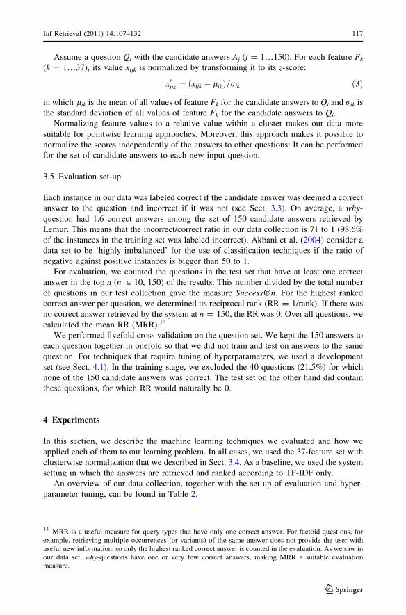
Assume a question Qi with the candidate answers Aj (j = 1…150). For each feature Fk

(k = 1…37), its value xijk is normalized by transforming it to its z-score:

x0ijk ¼ ðxijk � likÞ=rik ð3Þ

in which lik is the mean of all values of feature Fk for the candidate answers to Qi and rik is

the standard deviation of all values of feature Fk for the candidate answers to Qi.

Normalizing feature values to a relative value within a cluster makes our data more

suitable for pointwise learning approaches. Moreover, this approach makes it possible to

normalize the scores independently of the answers to other questions: It can be performed

for the set of candidate answers to each new input question.

3.5 Evaluation set-up

Each instance in our data was labeled correct if the candidate answer was deemed a correct

answer to the question and incorrect if it was not (see Sect. 3.3). On average, a why-

question had 1.6 correct answers among the set of 150 candidate answers retrieved by

Lemur. This means that the incorrect/correct ratio in our data collection is 71 to 1 (98.6%

of the instances in the training set was labeled incorrect). Akbani et al. (2004) consider a

data set to be ‘highly imbalanced’ for the use of classification techniques if the ratio of

negative against positive instances is bigger than 50 to 1.

For evaluation, we counted the questions in the test set that have at least one correct

answer in the top n (n [ 10, 150) of the results. This number divided by the total number

of questions in our test collection gave the measure Success@n. For the highest ranked

correct answer per question, we determined its reciprocal rank (RR = 1/rank). If there was

no correct answer retrieved by the system at n = 150, the RR was 0. Over all questions, we

calculated the mean RR (MRR).14

We performed fivefold cross validation on the question set. We kept the 150 answers to

each question together in onefold so that we did not train and test on answers to the same

question. For techniques that require tuning of hyperparameters, we used a development

set (see Sect. 4.1). In the training stage, we excluded the 40 questions (21.5%) for which

none of the 150 candidate answers was correct. The test set on the other hand did contain

these questions, for which RR would naturally be 0.

4 Experiments

In this section, we describe the machine learning techniques we evaluated and how we

applied each of them to our learning problem. In all cases, we used the 37-feature set with

clusterwise normalization that we described in Sect. 3.4. As a baseline, we used the system

setting in which the answers are retrieved and ranked according to TF-IDF only.

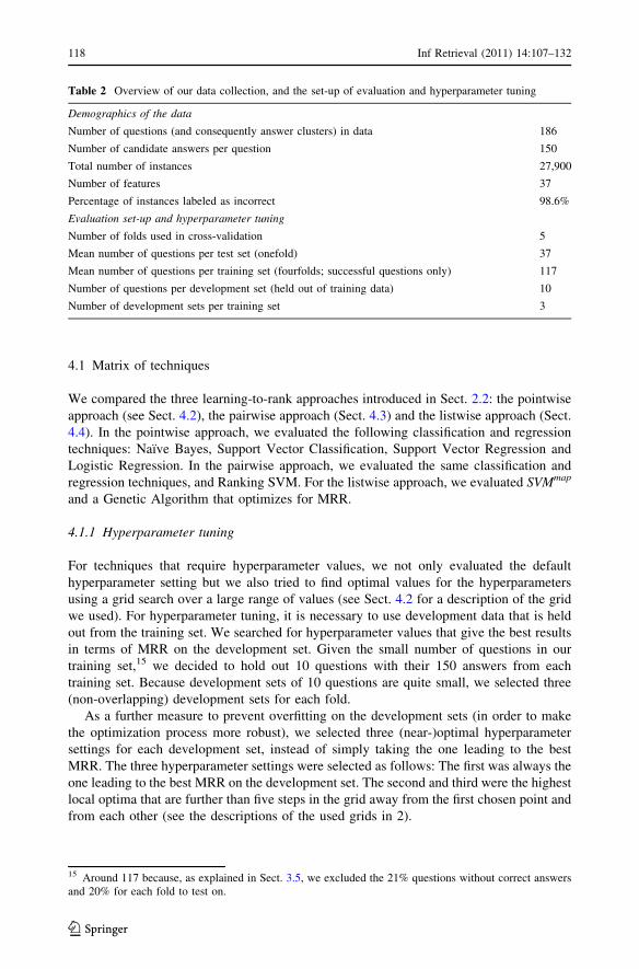
An overview of our data collection, together with the set-up of evaluation and hyper-

parameter tuning, can be found in Table 2.

14 MRR is a useful measure for query types that have only one correct answer. For factoid questions, forexample, retrieving multiple occurrences (or variants) of the same answer does not provide the user withuseful new information, so only the highest ranked correct answer is counted in the evaluation. As we saw inour data set, why-questions have one or very few correct answers, making MRR a suitable evaluationmeasure.

Inf Retrieval (2011) 14:107–132 117

123

4.1 Matrix of techniques

We compared the three learning-to-rank approaches introduced in Sect. 2.2: the pointwise

approach (see Sect. 4.2), the pairwise approach (Sect. 4.3) and the listwise approach (Sect.

4.4). In the pointwise approach, we evaluated the following classification and regression

techniques: Naı̈ve Bayes, Support Vector Classification, Support Vector Regression and

Logistic Regression. In the pairwise approach, we evaluated the same classification and

regression techniques, and Ranking SVM. For the listwise approach, we evaluated SVMmap

and a Genetic Algorithm that optimizes for MRR.

4.1.1 Hyperparameter tuning

For techniques that require hyperparameter values, we not only evaluated the default

hyperparameter setting but we also tried to find optimal values for the hyperparameters

using a grid search over a large range of values (see Sect. 4.2 for a description of the grid

we used). For hyperparameter tuning, it is necessary to use development data that is held

out from the training set. We searched for hyperparameter values that give the best results

in terms of MRR on the development set. Given the small number of questions in our

training set,15 we decided to hold out 10 questions with their 150 answers from each

training set. Because development sets of 10 questions are quite small, we selected three

(non-overlapping) development sets for each fold.

As a further measure to prevent overfitting on the development sets (in order to make

the optimization process more robust), we selected three (near-)optimal hyperparameter

settings for each development set, instead of simply taking the one leading to the best

MRR. The three hyperparameter settings were selected as follows: The first was always the

one leading to the best MRR on the development set. The second and third were the highest

local optima that are further than five steps in the grid away from the first chosen point and

from each other (see the descriptions of the used grids in 2).

Table 2 Overview of our data collection, and the set-up of evaluation and hyperparameter tuning

Demographics of the data

Number of questions (and consequently answer clusters) in data 186

Number of candidate answers per question 150

Total number of instances 27,900

Number of features 37

Percentage of instances labeled as incorrect 98.6%

Evaluation set-up and hyperparameter tuning

Number of folds used in cross-validation 5

Mean number of questions per test set (onefold) 37

Mean number of questions per training set (fourfolds; successful questions only) 117

Number of questions per development set (held out of training data) 10

Number of development sets per training set 3

15 Around 117 because, as explained in Sect. 3.5, we excluded the 21% questions without correct answersand 20% for each fold to test on.

118 Inf Retrieval (2011) 14:107–132

123

During testing, the outputs of the nine models that were created for the three devel-

opment sets (three models per development set) were combined by addition, after scaling

them to a comparable range.

4.2 The pointwise approach

We first investigated the pointwise approach of applying classification and regression

techniques to our learning problem. In the training phase, the classifier or regressor learns

to classify each instance (question answer pair) as either correct or incorrect, irrespective

of the cluster it belongs to.16 In the test phase, we let the model assign a score to each

instance in the data representing the likelihood that this instance should be classified as

correct. The actual ranking is done by a script that sorts the instances per cluster by the

output score of the classifier.

As discussed in Sect. 3.5, our data show a strong imbalance between positive and

negative instances, with a incorrect/correct ratio of 71. This may cause problems for

machine learning techniques that are designed for classification. Therefore, we applied a

balancing strategy to all classification and regression techniques that we evaluated. As

observed in the literature (Japkowicz and Stephen 2002; Tang et al. 2009), applying a cost

factor is the preferred approach to counter imbalance. If a system did not allow for this, we

applied oversampling of the positive instances in such a way that each training set included

approximately as many positive as negative instances.

In the pointwise approach, we trained and tested each machine learning technique both

on the original (imbalanced) data and on the data that was balanced first (by applying a cost

factor or oversampling). For the classifiers that allow for hyperparameter optimization, we

performed the optimization for both these data variants. This led to two (when hyperpa-

rameter optimization is not feasible) or four different settings per machine learning

technique: original default, original tuned, balanced default, and balanced tuned.

4.2.1 Naı̈ve Bayes classifier (NB)

For experiments with Naı̈ve Bayes (NB), we used the e1071 package in R.17 This package

does not allow for tuning of hyperparameters for Naı̈ve Bayes so we only ran the Naı̈ve

Bayes classifier in its default setting, on both the original and the oversampled data.

4.2.2 Support vector classification and support vector regression (SVR)

For standard support vector methods, we used LIBSVM.18 As proposed by the authors of

LIBSVM, we first scaled our data using svm-scale. We experimented with support vector

classification (C-SVC) and support vector regression (e-SVR). For both, we used the RBF

kernel (Hsu et al. 2003).

The RBF kernel expects two hyperparameters: c—the trade-off between training error

and margin, and c—a multiplication factor determining the range of kernel space vector

norms. Their default values are c = 1 and c = 1/k with k being the number of features,

giving a c of 0.027 for our data. For the grid search, we followed the suggestion in Hsu

16 Recall that we did normalize the feature values per cluster, which made our data more suitable forpointwise learning approaches.17 See http://www.cran.r-project.org/web/packages/e1071/index.html.18 See http://www.csie.ntu.edu.tw/*cjlin/libsvm.

Inf Retrieval (2011) 14:107–132 119

123

et al. (2003) to use exponentially growing sequences of c and c. We varied c from 2-13 to

213 in steps of 92 and c from 2-13 to 27 in steps of 94.19

Support vector classification allows us to use a cost factor for training errors on positive

instances, which we did: During hyperparameter tuning, we kept the cost factor unchanged

at 71 (-w1 = 71). For SVR (which does not allow for a cost factor), we oversampled the

positive instances in the training sets.

4.2.3 Logistic regression (LRM)

We used the lrm function from the Design package in R for training and evaluating

models based on logistic regression.20 LRM uses Maximum Likelihood Estimation (MLE)

as optimization function. We used ‘correct’ and ‘incorrect’ as target values in the training

phase. In the test phase, the regression function is applied to the instances in the test set,

predicting for each item the log odds that it should be categorized as ‘correct’.

LRM has a built-in option for data balancing (applying a weight vector to all instances),

of which we found that it has exactly the same effect on the data as oversampling the

positive instances in the training set. The other hyperparameters in LRM (a parameter for

handling collinearity in stepwise approaches21 and a penalty parameter for data with many

features and relatively few instances) are not relevant for our data. Therefore, we refrained

from hyperparameter tuning for LRM: We only trained models using the default parameter

settings for both the original and the balanced data.

4.3 The pairwise approach

For the pairwise approach, we evaluated Joachim’s algorithm Ranking SVM (Joachims

2002). In addition, we evaluated the same classification and regression techniques as in the

pointwise approach. We made this possible by transforming our data into instance pairs

that can be handled by these techniques (as explained below).

4.3.1 Ranking SVM

We used version 6 of SVMlight for our Ranking SVM experiments.22 Ranking SVM con-

siders the training data to be a set of instance pairs, each pair consisting of one correct and

one incorrect answer. On these instances, the system performs pairwise preference learning

(Joachims 2002). The ranking order of a set of training instances is optimized according to

Kendall Tau:

s ¼ ðNc � NdÞðNc þ NdÞ

ð4Þ

in which Nc is the number of concordant item pairs (the two items are ordered cor-

rectly) and Nd is the number of discordant item pairs (the two items are ordered

incorrectly).

19 This means that each next value is 4 times as high as the previous, so we go from 2-13 to 2-11 to 2-9, etc.20 See http://www.cran.r-project.org/web/packages/Design/index.html.21 We only built regression models that contained all features as predictors.22 See http://www.svmlight.joachims.org.

120 Inf Retrieval (2011) 14:107–132

123

Similar to the other SVM techniques, we used the RBF kernel in Ranking SVM, which

takes both the hyperparameters c and c. For both, the default value is 1. For tuning these

parameters, we searched over the same grid as for SVC.

4.3.2 Classification and regression techniques

To enable the use of other classifiers than Ranking SVM and regression techniques in a

pairwise approach, we transformed our data into a set of instance pairs, similarly to the

approach implemented by Joachims in Ranking SVM. We presented the answers in pairs of

one correct and one incorrect answer to the same question. We kept the number of features

constant (at 37), but we transformed each feature value to the difference between the

values of the two answers in the pair. In other words, we created feature vectors consisting

of 37 difference values.

In the training data, each instance pair is included twice: ‘correct minus incorrect’ with

label ‘correctly ordered’ and ‘incorrect minus correct’ with label ‘incorrectly ordered’. In

the testing phase, we let the classifier assign to each instance pair the probability that it is

correctly ordered. Then we transform the data back to normal answer instances by sum-

ming the scores for each answer i over all pairs [i, j] in which i is ranked first.

We evaluated the same classifiers and regression techniques in the pairwise approach as

we evaluated for the pointwise approach: Naı̈ve Bayes, Support Vector Classification,

Support Vector Regression and Logistic Regression. Although our implementation of

pairwise classification for SVC is conceptually equal to Ranking SVM, there are some

implementational differences (such as the use of LIBSVM vs. SVMlight).23 We decided to

evaluate both so that we could maintain a link to previous work as well as get more direct

comparability with the other pairwise classification and regression methods.

4.4 The listwise approach

In the listwise approach there is no classification of instances or instance pairs; instead, the

ordering of an answer cluster as a whole is optimized. As explained in Sect. 2.2, the

implementation of listwise ranking approaches is a recent development and the results

obtained with these techniques are promising (Yue et al. 2007; Xu and Li 2007). We

evaluated two listwise optimization algorithms: SVMmap, and our own implementation of a

genetic algorithm that optimizes the order of answers per question using MRR as fitness

function.24

4.4.1 SVMmap

SVMmap is a freely available algorithm25 that takes clusters of instances with binary rel-

evance labels as input and optimizes the instance order within each cluster for Mean

Average Precision (MAP) (Yue et al. 2007). Average precision is calculated as:

23 The default value for c is 1/k in LIBSVM and 1 in SVMlight.24 To our knowledge, there are no implementations of AdaRank and ListNet available for download and toexperiment with.25 See http://www.projects.yisongyue.com/svmmap.

Inf Retrieval (2011) 14:107–132 121

123

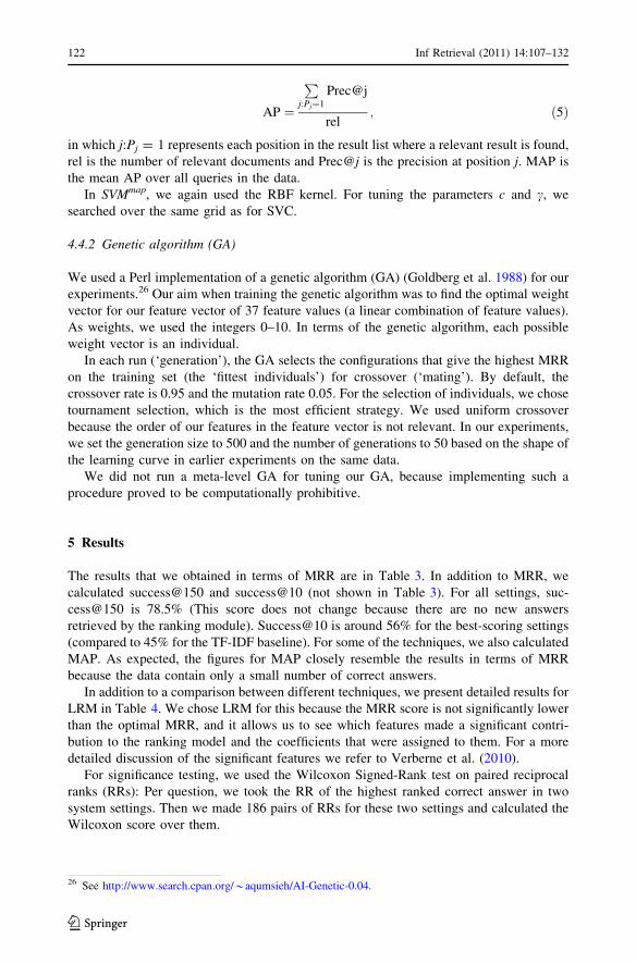
AP ¼

P

j:Pj¼1

Prec@j

rel; ð5Þ

in which j:Pj = 1 represents each position in the result list where a relevant result is found,

rel is the number of relevant documents and Prec@j is the precision at position j. MAP is

the mean AP over all queries in the data.

In SVMmap, we again used the RBF kernel. For tuning the parameters c and c, we

searched over the same grid as for SVC.

4.4.2 Genetic algorithm (GA)

We used a Perl implementation of a genetic algorithm (GA) (Goldberg et al. 1988) for our

experiments.26 Our aim when training the genetic algorithm was to find the optimal weight

vector for our feature vector of 37 feature values (a linear combination of feature values).

As weights, we used the integers 0–10. In terms of the genetic algorithm, each possible

weight vector is an individual.

In each run (‘generation’), the GA selects the configurations that give the highest MRR

on the training set (the ‘fittest individuals’) for crossover (‘mating’). By default, the

crossover rate is 0.95 and the mutation rate 0.05. For the selection of individuals, we chose

tournament selection, which is the most efficient strategy. We used uniform crossover

because the order of our features in the feature vector is not relevant. In our experiments,

we set the generation size to 500 and the number of generations to 50 based on the shape of

the learning curve in earlier experiments on the same data.

We did not run a meta-level GA for tuning our GA, because implementing such a

procedure proved to be computationally prohibitive.

5 Results

The results that we obtained in terms of MRR are in Table 3. In addition to MRR, we

calculated success@150 and success@10 (not shown in Table 3). For all settings, suc-

cess@150 is 78.5% (This score does not change because there are no new answers

retrieved by the ranking module). Success@10 is around 56% for the best-scoring settings

(compared to 45% for the TF-IDF baseline). For some of the techniques, we also calculated

MAP. As expected, the figures for MAP closely resemble the results in terms of MRR

because the data contain only a small number of correct answers.

In addition to a comparison between different techniques, we present detailed results for

LRM in Table 4. We chose LRM for this because the MRR score is not significantly lower

than the optimal MRR, and it allows us to see which features made a significant contri-

bution to the ranking model and the coefficients that were assigned to them. For a more

detailed discussion of the significant features we refer to Verberne et al. (2010).

For significance testing, we used the Wilcoxon Signed-Rank test on paired reciprocal

ranks (RRs): Per question, we took the RR of the highest ranked correct answer in two

system settings. Then we made 186 pairs of RRs for these two settings and calculated the

Wilcoxon score over them.

26 See http://www.search.cpan.org/*aqumsieh/AI-Genetic-0.04.

122 Inf Retrieval (2011) 14:107–132

123

Table 3 Results for the pointwise, pairwise and listwise approaches in terms of MRR

Technique Pointwise approach

Original default Original tuned Balanced default Balanced tuned

TF-IDF 0.25

NB 0.19 – 0.20 –

SVC 0.10 0.32*,� 0.32*,� 0.33*,�

SVR 0.34*,� 0.30* 0.33*,� 0.32*,�

LRM 0.34*,� – 0.31* –

Technique Pairwise approach

Default Tuned

NB 0.32*,� –

SVC 0.32*,� 0.34*,�

SVR 0.32*,� 0.35*

LRM 0.31* –

Ranking SVM 0.13 0.33*,�

Technique Listwise approach

Default Tuned

GA-MRR 0.32*,� –

SVMmap 0.33*,� 0.34*,�

The highest score is printed in boldface. An asterisk (*) on an MRR score indicates a statistically significantimprovement (P \ 0.01 according to the Wilcoxon signed-rank test) over the TF-IDF baseline. A dagger (�)indicates that the MRR score is not significantly lower than the highest MRR score (0.35)

Table 4 Detailed results for LRM on original data in terms of MRR, MAP, Success@10, Success@150,and the coefficients of the features that significantly contribute to the re-ranking score (P \ 0.05), ranked bytheir coefficient in LRM (representing their strength)

Mean reciprocal rank (MRR) 0.34

Mean average precision (MAP) 0.32

Success@10 57.0%

Success@150 78.5%

Significant features Coefficient

TF-IDF 0.39**

Overlap between question focus synonyms and document title 0.25**

Overlap between question object synonyms and answer words 0.22

Overlap between question object and answer objects 0.18*

Overlap between question words and document title synonyms 0.17

Overlap between question verb synonyms and answer words 0.16

WordNet Relatedness 0.16*

Cue phrases 0.15*

Asterisks on coefficients denote the level of significance for the feature: ** means P \ 0.001, * means0.001 \ P \ 0.01, no asterisk means 0.01 \ P \ 0.05

Inf Retrieval (2011) 14:107–132 123

123

The highest MRR score that we obtained is 0.35 (by SVR for pairwise classification).27

We will call this the optimum in the remainder of this section.

5.1 Comparing pointwise, pairwise and listwise approaches

We obtained good results with techniques following either of the three approaches:

pointwise, pairwise and listwise. The results for the pairwise approach much resemble the

results for balanced data in the pointwise approach. This finding confirms the results found

by other researchers on LETOR data: pairwise approaches are in some cases slightly better

than pointwise approaches but pointwise approaches can reach good results if the data are

balanced and the hyperparameters are tuned properly.

For Naı̈ve Bayes, however, the results for the pointwise and pairwise approaches are

very different. Here we see that presenting the problem as a pairwise classification problem

is essential for Naı̈ve Bayes to predict the data correctly. We suspect that this is because the

simplicity of the Naı̈ve Bayes model, which is based on the probability of each feature

value given the class of the instance. When presenting the data in pairs, we apply a form of

bagging: Each positive answer is included in the data many times, but each time as part of

a different instance pair. As a result, all positive instance pairs are different from each other

and the algorithm has more more quasi-independent data points available for learning to

make the right decision for one answer. Not surprisingly, the Naı̈ve Bayes classifier

depends on the availability of (quasi-)independent training data for learning a proper

classifier.

In the bottom part of Table 3, we see that both our listwise approaches (GA-MRR and

SVMmap) lead to scores that are not significantly lower than the optimum, but also not

higher than the results for the pointwise and pairwise techniques. From the literature on

listwise techniques one would expect a result that is better than the pointwise and pairwise

approaches. We speculate that the failure of our GA approach to outperform pointwise and

pairwise approaches is because the linear feature combination with integer weights that we

implemented in the Genetic Algorithm is not sophisticated enough for learning the data

properly. The results for SVMmap may be suboptimal because the optimization is done on a

different function (MAP) than the evaluation measure (MRR). We [and others (Liu 2009)]

have found before that the best results with listwise techniques are obtained with a loss

function that optimally resembles the evaluation measure. In that respect, it would be

interesting to experiment with the lesser known algorithm SVMmrr (Chakrabarti et al.

2008).

5.2 The effect of data imbalance

As pointed out in the machine learning literature (see Sect. 2.3), classifiers are in general

sensitive to data imbalance. Table 3 shows that especially pointwise SVC gives very poor

results in its default setting on our imbalanced data. If we balance the data, SVC reaches

good results with the default settings of LIBSVM. As opposed to SVC, the results for

Naı̈ve Bayes are not improved by balancing the data.

27 The 21% of questions without a correct answer in the top 150 all have an RR of 0; the MRR for thesuccessful questions only is 0.45. This is quite high considering the Success@10 score of 56%. A furtherinvestigation of the results shows us that this is because a large proportion of successful questions has acorrect answer at position 1 (Success@1 for all questions including the unsuccessful questions is 24.2%).

124 Inf Retrieval (2011) 14:107–132

123

We find that for regression techniques (SVR and LRM), balancing the data by over-

sampling or applying a cost factor leads to slightly (not significantly) lower MRR scores. In

Sect. 6.2 we provide an analysis of the regression models for the original and balanced

data.

5.3 The effect of hyperparameter tuning

The effects of hyperparameter tuning on the ability of a technique to model our data varies

much between the different techniques. The results for pointwise SVC show that with

optimal hyperparameter settings SVC is able to reach a good result, even for the highly

imbalanced data, on which the default settings performed very poorly. Ranking SVM, for

which the default settings also give a result below baseline, also profits significantly from

hyperparameter optimization (P \ .0001).

On the other hand, for those settings where default hyperparameters already give good

results (most pointwise approaches on the balanced data and most pairwise approaches),

we see that hyperparameter tuning does not lead to significantly better MRR scores. The

only exception is pairwise SVR with P = 0.01 according to Wilcoxon.

There is one setting where we even observe a significant (P = 0.0003) lower MRR

score after hyperparameter tuning compared to the default setting: pointwise SVR on the

original data. In Sect. 6.3, we will provide an analysis of the tuning process in order to see

if our experiments suffer from overfitting. Additionally, we will analyze the differences

between individual questions in Sect. 6.4.

6 Discussion

6.1 Relating our findings to previous work

Although our feature set is different from the feature sets that are used in previous work on

learning to rank for Information Retrieval, there are also similarities between our data and

more commonly used data in learning-to-rank research: in all data, the instances are

clustered by query, and there is often a strong imbalance between positive and negative

instances.

The performance differences that we find between pointwise, pairwise and listwise

approaches are small, especially after balancing the data. We argue that this is largely in

line with earlier findings in learning-to-rank for Information Retrieval, where differences

between the three approaches on smaller datasets are not always significant (Liu 2009).

We can identify four distinct reasons why some of our findings are different from the

findings in the learning-to-rank literature. First of all, our data collection is relatively small

(186 questions), as a result of which it is difficult to get differences that are statistically

significant. The same pattern of listwise methods being not significantly better than pair-

wise and pointwise methods can be observed for some of the smaller LETOR collections

such as OHSUMED, which contains only 106 queries (Liu et al. 2007).

Secondly, we performed clusterwise normalization on the data for all techniques. As a

result, the feature values of one candidate answer in the training set are related to the

feature values of other candidate answers to the same question. This gives pointwise

techniques ‘awareness’ of the clustering of the answers per question. Thirdly, in hyper-

parameter tuning, we optimized for MRR on the development set. This means that all

techniques profit from the advantage of optimizing for the measure that is used for

Inf Retrieval (2011) 14:107–132 125

123

evaluation as well. Finally, the listwise techniques that we evaluated are suboptimal: the

genetic algorithm only performs a linear combination of feature values using integer

weights; SVMmap optimizes for a different measure than our main evaluation measure.

6.2 Analyzing the effect of data imbalance

In Sect. 5.2, we found that for regression techniques, balancing the data by oversampling or

applying a cost factor leads to slightly (not significantly) lower MRR scores. In Sect. 2.3,

we concluded from the literature that class imbalance causes fewer problems for regression

techniques than for classifiers because in the regression model, the intercept value moves

the outcome of the regression function towards the bias in the data.

An analysis of the regression models that were created by LRM for the original and the

balanced data showed that the model for the balanced data contains much more significant

effects (features that significantly contribute to the ranking model) than the model for the

original data. Due to oversampling the positive instances in the training set, the regression

function was strongly influenced by the heavy data points that each represent 71 positive

instances. Misclassifying some of the negative instances during training does not influence

the model fit too badly because there are much more positive data points. However, when

applying the model to generate a ranking, the few negative instances that are misclassified

are ranked above the positive instances. The MRR, which only considers the positive

instance that is ranked highest, has therefore decreased.

6.3 Analyzing the effect of hyperparameter tuning

In Sect. 5.3, we reported that for those settings where default hyperparameters already give

good results, hyperparameter tuning does not lead to better MRR scores. To examine

whether overfitting on the development sets was the cause of this, we analyzed the results

for one of the methods where a slight deterioration in MRR was observed between default

and tuned hyperparameter settings: pointwise SVR on balanced data. For this setting, we

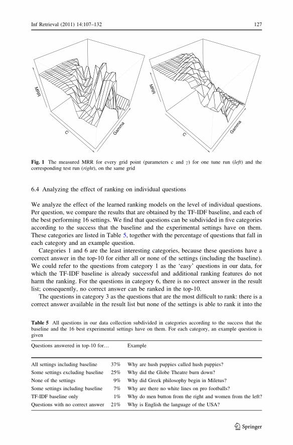
plotted the measured MRR for every grid point for all tune and test runs. We then com-

pared the surfaces for corresponding tune and test runs.

In the ideal situation, the surfaces would not need to coincide, but at least the highest

peaks should be close to each other in the grid. Although this is the case for a few runs, the

typical situation is that in Fig. 1, where the tune and test surfaces for fold 4, development

set A are shown. The grid area where the peak occurs in the tune run has a lower than

average MRR in the test run.

We also observe that the surfaces are not very smooth and sometimes show strong local

jumps. This means that for a determination of the real optimal hyperparameters for each

run, a denser grid would be preferable. However, seeing the mismatch between the surfaces

for tune and test runs, we expect that this would not solve the problem of lower MRR

scores after tuning. Thus, the process of hyperparameter tuning is hampered by the

sparseness of our data.

The large differences between the optimal hyperparameter values that are found for

different development sets shows that the optimal hyperparameter values are highly

influenced by the individual questions in each development set. We conclude that for

tuning purposes, a development set size of ten questions is clearly too small. Our strategy

of using three development sets per training set has probably alleviated, but certainly not

solved this problem.

126 Inf Retrieval (2011) 14:107–132

123

6.4 Analyzing the effect of ranking on individual questions

We analyze the effect of the learned ranking models on the level of individual questions.

Per question, we compare the results that are obtained by the TF-IDF baseline, and each of

the best performing 16 settings. We find that questions can be subdivided in five categories

according to the success that the baseline and the experimental settings have on them.

These categories are listed in Table 5, together with the percentage of questions that fall in

each category and an example question.

Categories 1 and 6 are the least interesting categories, because these questions have a

correct answer in the top-10 for either all or none of the settings (including the baseline).

We could refer to the questions from category 1 as the ‘easy’ questions in our data, for

which the TF-IDF baseline is already successful and additional ranking features do not

harm the ranking. For the questions in category 6, there is no correct answer in the result

list; consequently, no correct answer can be ranked in the top-10.

The questions in category 3 as the questions that are the most difficult to rank: there is a

correct answer available in the result list but none of the settings is able to rank it into the

C Gam

ma

MR

R

C

Gam

ma

MR

R

Fig. 1 The measured MRR for every grid point (parameters c and c) for one tune run (left) and thecorresponding test run (right), on the same grid

Table 5 All questions in our data collection subdivided in categories according to the success that thebaseline and the 16 best experimental settings have on them. For each category, an example question isgiven

Questions answered in top-10 for… Example

All settings including baseline 37% Why are hush puppies called hush puppies?

Some settings excluding baseline 25% Why did the Globe Theatre burn down?

None of the settings 9% Why did Greek philosophy begin in Miletus?

Some settings including baseline 7% Why are there no white lines on pro footballs?

TF-IDF baseline only 1% Why do men button from the right and women from the left?

Questions with no correct answer 21% Why is English the language of the USA?

Inf Retrieval (2011) 14:107–132 127

123

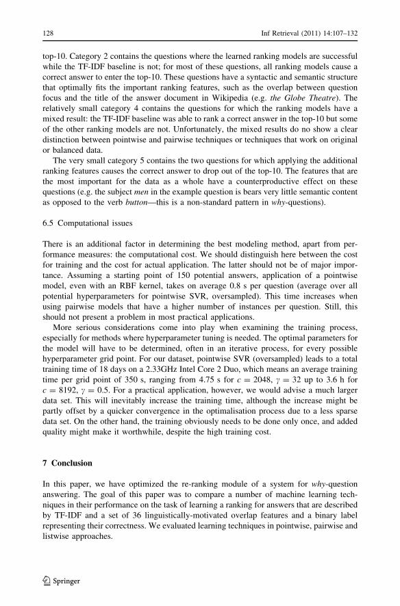
top-10. Category 2 contains the questions where the learned ranking models are successful

while the TF-IDF baseline is not; for most of these questions, all ranking models cause a

correct answer to enter the top-10. These questions have a syntactic and semantic structure

that optimally fits the important ranking features, such as the overlap between question

focus and the title of the answer document in Wikipedia (e.g. the Globe Theatre). The

relatively small category 4 contains the questions for which the ranking models have a

mixed result: the TF-IDF baseline was able to rank a correct answer in the top-10 but some

of the other ranking models are not. Unfortunately, the mixed results do no show a clear

distinction between pointwise and pairwise techniques or techniques that work on original

or balanced data.

The very small category 5 contains the two questions for which applying the additional

ranking features causes the correct answer to drop out of the top-10. The features that are

the most important for the data as a whole have a counterproductive effect on these

questions (e.g. the subject men in the example question is bears very little semantic content

as opposed to the verb button—this is a non-standard pattern in why-questions).

6.5 Computational issues

There is an additional factor in determining the best modeling method, apart from per-

formance measures: the computational cost. We should distinguish here between the cost

for training and the cost for actual application. The latter should not be of major impor-

tance. Assuming a starting point of 150 potential answers, application of a pointwise

model, even with an RBF kernel, takes on average 0.8 s per question (average over all

potential hyperparameters for pointwise SVR, oversampled). This time increases when

using pairwise models that have a higher number of instances per question. Still, this

should not present a problem in most practical applications.

More serious considerations come into play when examining the training process,

especially for methods where hyperparameter tuning is needed. The optimal parameters for

the model will have to be determined, often in an iterative process, for every possible

hyperparameter grid point. For our dataset, pointwise SVR (oversampled) leads to a total

training time of 18 days on a 2.33GHz Intel Core 2 Duo, which means an average training

time per grid point of 350 s, ranging from 4.75 s for c = 2048, c = 32 up to 3.6 h for

c = 8192, c = 0.5. For a practical application, however, we would advise a much larger

data set. This will inevitably increase the training time, although the increase might be

partly offset by a quicker convergence in the optimalisation process due to a less sparse

data set. On the other hand, the training obviously needs to be done only once, and added

quality might make it worthwhile, despite the high training cost.

7 Conclusion

In this paper, we have optimized the re-ranking module of a system for why-question

answering. The goal of this paper was to compare a number of machine learning tech-

niques in their performance on the task of learning a ranking for answers that are described

by TF-IDF and a set of 36 linguistically-motivated overlap features and a binary label

representing their correctness. We evaluated learning techniques in pointwise, pairwise and

listwise approaches.

128 Inf Retrieval (2011) 14:107–132

123

We found that with all machine learning techniques, we can get to an MRR score that is

significantly above the TF-IDF baseline of 0.25 and not significantly lower than the best

score of 0.35.

We are able to obtain good results with all three types of approaches for our data:

pointwise, pairwise and listwise. The optimum score was reached by Support Vector

Regression for the pairwise representation, but some of the pointwise settings reached

scores that were not significantly lower than this optimum. We argue that pointwise

approaches can reach good results for learning-to-rank problems if (a) data imbalance is

solved before training by applying a cost factor or oversampling the positive instances, (b)

feature value normalization is applied per answer cluster (query-level normalization) and/

or (c) proper hyperparameter tuning is performed.

We obtained reasonable results with two listwise techniques: SVMmap and a Genetic

Algorithm (GA) optimizing for MRR. With these techniques, we obtained results that are

comparable to those obtained with the pointwise and pairwise approaches. Given our

suboptimal choice of optimization function (SVMmap vs. SVMmrr) and our relatively simple

implementation with a linear combination of feature values in the GA, we think that our

results confirm the earlier findings that listwise approaches to learning-to-rank are

promising.

We found that for our imbalanced data set, some of the techniques with hyperparam-

eters heavily depend on tuning. However, if we solve the class imbalance by balancing our

data or presenting the problem as a pairwise classification task then the default hyperpa-

rameter values are well applicable to the data and tuning is less important. The pairwise

transformation enables even Naı̈ve Bayes to classify and rank the data properly. Since

hyperparameter tuning is a process that takes much time and computational power, a

technique without hyperparameters, or a technique for which tuning can be done easily

without heavy computing, should be preferred if it reaches equal performance to tech-

niques with (more heavy) tuning. In this respect, regression techniques seem the best

option for our learning problem: logistic regression reaches a score very close to the

optimum (MRR is 0.34) without tuning. Pairwise support vector regression reaches optimal

performance (MRR is 0.35) with tuning.

It seems that with the current feature set we have reached a ceiling as far as individual

rankers are concerned. We might still achieve an improvement with a combination of

rankers or second level classifiers, but the overlap between the results for individual

systems is such that this improvement can never be very big.28

Moreover, given the experimental result of 0.35 and the theoretical optimum of 0.79 (if

for all questions with at least one correct answer a correct answer is ranked at position 1),

we can conclude that our features are suboptimal for distinguishing correct from incorrect

answers. Since we already invested much time in previous work in finding the best features

for describing our data, we conclude that the problem of distinguishing correct and

incorrect answers to why-questions is more complex than an approach based on textual

(overlap) features can solve.

Our future work will review the problem of answering why-questions in detail. In

automatically answering complex questions such as why-questions, human reasoning and

28 In fact, we did some preliminary experiments with a linear combination of answer scores from combi-nations of rankers. By use of a hill-climbing mechanism we were able to find a set of weights that leads to anMRR on the test set of 0.38. This is significantly better than the best-scoring individual technique(P = 0.03). We have not attempted second level classification, since this would mean repeating all ourexperiments with a nested cross-validation in order to do a proper training and tuning of the second levelclassifier.

Inf Retrieval (2011) 14:107–132 129

123

world knowledge seem to play an important role. We will investigate the limitations of an

Information Retrieval-based approach that relies on word overlap for complex question

answering.

Open Access This article is distributed under the terms of the Creative Commons Attribution Noncom-mercial License which permits any noncommercial use, distribution, and reproduction in any medium,provided the original author(s) and source are credited.

References

Akbani, R., Kwek, S., & Japkowicz, N. (2004). Applying support vector machines to imbalanced datasets. InLecture notes in computer science: Machine learning: ECML 2004 (Vol. 3201, pp. 39–50). New York:Springer.

Aslam, J. A., Kanoulas, E., Pavlu, V., Savev, S., & Yilmaz, E. (2009). Document selection methodologiesfor efficient and effective learning-to-rank. In Proceedings of the 32nd annual international ACMSIGIR conference on research and development in information retrieval (pp. 468–475). New York,NY: ACM.

Banerjee, S., & Pedersen, T. (2002). An adapted Lesk algorithm for word sense disambiguation usingWordNet. In Lecture notes in computer science: Computational linguistics and intelligent text pro-cessing (pp. 136–145). New York: Springer.

Burges, C., Shaked, T., Renshaw, E., Lazier, A., Deeds, M., Hamilton, N., et al. (2005). Learning to rankusing gradient descent. In Proceedings of the 22nd international conference on machine learning(pp. 89–96)

Cao, Z., Qin, T., Liu, T., Tsai, M., & Li, H. (2007). Learning to rank: from pairwise approach to listwiseapproach. In Proceedings of the 24th international conference on machine learning (pp. 129–136).New York, NY: ACM.

Carterette, B., & Petkova, D. (2006). Learning a ranking from pairwise preferences. In Proceedings of the29th annual international ACM SIGIR conference on research and development in informationretrieval (pp. 629–630). New York, NY: ACM.

Chakrabarti, S., Khanna, R., Sawant, U., & Bhattacharyya, C. (2008). Structured learning for non-smoothranking losses. In Proceedings of the 14th ACM SIGKDD international conference on knowledgediscovery and data mining (pp. 88–96). New York, NY: ACM.

Charniak, E. (2000). A maximum-entropy-inspired parser. ACM International Conference ProceedingsSeries, 4, 132–139.

Cossock, D., & Zhang, T. (2006) Subset ranking using regression. In Lecture notes in computer science:Learning theory (Vol. 4005, p. 605). New York: Springer.

Denoyer, L., & Gallinari, P. (2006). The Wikipedia XML corpus. ACM SIGIR Forum, 40(1), 64–69.Fan, W., Fox, E., Pathak, P., & Wu, H. (2004). The effects of fitness functions on genetic programming-

based ranking discovery for web search. Journal of the American Society for Information Science andTechnology, 55(7), 628–636.

Fellbaum, C. (eds) (1998) WordNet: An electronic lexical database. Cambridge, MA: MIT Press.Freund, Y., Iyer, R., Schapire, R., & Singer, Y. (2003). An efficient boosting algorithm for combining

preferences. The Journal of Machine Learning Research, 4, 933–969.Furnkranz, J., & Hullermeier, E. (2003). Pairwise preference learning and ranking. In Lecture notes in

computer science: Machine learning: ECML 2003 (pp. 145–156). New York: Springer.Goldberg, D., & Holland, J. (1988). Genetic algorithms and machine learning. Machine Learning, 3(2), 95–99Herbrich, R., Graepel, T., & Obermayer, K. (2002). Large margin rank boundaries for ordinal regression. In

Proceedings of the 8th ACM SIGKDD international conference on knowledge discovery and datamining (pp. 133–142). New York, NY: ACM.

Higashinaka, R., & Isozaki, H. (2008). Corpus-based question answering for why-questions. In Proceedingsof the international joint conference on natural language processing (IJCNLP) (pp. 418–425).

Hovy, E., Hermjakob, U., & Ravichandran, D. (2002). A question/answer typology with surface textpatterns. In Proceedings of the human language technology conference (HLT), San Diego, CA, USA,pp. 247–251.

Hsu, C., Chang, C., & Lin, C., et al. (2003). A practical guide to support vector classification. Technicalreport, Department of Computer Science, National Taiwan University, Taipei 106, Taiwan.

130 Inf Retrieval (2011) 14:107–132

123

Japkowicz, N., & Stephen, S. (2002). The class imbalance problem: A systematic study. Intelligent DataAnalysis, 6(5), 429–449.

Joachims, T. (2002) Optimizing search engines using clickthrough data. In Proceedings of the 8th ACMSIGKDD international conference on knowledge discovery and data mining (pp. 133–142). New York,NY: ACM.

Liu, T. (2009). Learning to rank for information retrieval. Foundations and Trends in Information Retrieval,3(3), 225–331.

Liu, T., Xu, J., Qin, T., Xiong, W., & Li, H. (2007). Letor: Benchmark dataset for research on learning torank for information retrieval. In Proceedings of the workshop on learning to rank for informationretrieval (LR4IR) at SIGIR 2007 (pp. 3–10).

Maybury, M. (2002). Toward a question answering roadmap. Technical report, Mitre Corporation, Bedford,MA, USA.

Owen, A. (2007). Infinitely imbalanced logistic regression. The Journal of Machine Learning Research, 8,761–77.

Pedersen, T., Patwardhan, S., & Michelizzi, J. (2004). WordNet::Similarity—Measuring the relatedness ofconcepts. In Proceedings of the national conference on artificial intelligence (pp. 1024–1025). MenloPark: AAAI Press.

Qin, T., Liu, T., Xu, J., & Li, H. (2008) LETOR: A benchmark collection for learning to rank for infor-mation retrieval. Technical report, Microsoft Research Asia

Shen, L., & Joshi, A. (2005). Ranking and reranking with perceptron. Machine Learning, 60(1), 73–96.Surdeanu, M., Ciaramita, M., & Zaragoza, H. (2008). Learning to rank answers on large online QA

collections. In Proceedings of the 46th annual meeting on association for computational linguistics(pp. 719–727).

Tang, Y., Zhang, Y., Chawla, N., & Krasser, S. (2009). SVMs modeling for highly imbalanced classifi-cation. IEEE Transactions on Systems, Man, and Cybernetics, Part B, 39(1), 281–288.

Tiedemann, J. (2007). A comparison of genetic algorithms for optimizing linguistically informed IR inquestion answering. In Lecture notes in computer science: AI*IA 2007: Artificial intelligence andhuman-oriented computing (Vol. 4733, pp. 398). New York: Springer.

Trotman, A. (2004). An artificial intelligence approach to information retrieval. In Proceedings of the 27thannual international ACM SIGIR conference on research and development in information retrieval(p. 603). New York, NY: ACM.

Usunier, N., Amini, M., & Gallinari, P. (2004). Boosting weak ranking functions to enhance passageretrieval for question answering. In Proceedings of the workshop on information retrieval for questionanswering (IR4QA) at SIGIR 2004 (pp. 1–6).

Verberne, S., Boves, L., Oostdijk N., & Coppen, P. (2007). Evaluating discourse-based answer extraction forwhy-question answering. In Proceedings of the 30th annual international ACM SIGIR conference onresearch and development in information retrieval (pp. 735–736). New York, NY: ACM.

Verberne, S., Boves, L., Oostdijk, N., & Coppen, P. (2008). Using syntactic information for improving why-question answering. In Proceedings of the 22nd international conference on computational linguistics(COLING) (pp. 953–960).

Verberne, S., Boves, L., Oostdijk, N., & Coppen, P. (2010). What is not in the bag of words for why-QA?Computational Linguistics, 32(2), 229–245.

Voorhees, E. (2000). Overview of the TREC-9 question answering track. In Proceedings of TREC-9 (Vol. 7,pp. 1–80).

Voorhees, E. (2003). Overview of the TREC 2003 question answering track. In Proceedings of the twelfthtext retrieval conference (TREC 2003) (Vol. 142, pp. 54–68).

Voorhees, E., & Tice, D. (2000). Building a question answering test collection. In Proceedings of the 23rdannual international ACM SIGIR conference on research and development in information retrieval(pp. 200–207). New York, NY: ACM.

Xia, F., Liu, T., Wang, J., Zhang, W., & Li, H. (2008). Listwise approach to learning to rank: Theory andalgorithm. In Proceedings of the 25th international conference on machine learning (pp. 1192–1199).New York, NY: ACM

Xu, J., & Li, H. (2007) Adarank: A boosting algorithm for information retrieval. In Proceedings of the 30thannual international ACM SIGIR conference on research and development in information retrieval(pp. 391–398). New York, NY: ACM.

Yeh, J., Lin, J., Ke, H., Yang, W. (2007). Learning to rank for information retrieval using genetic pro-gramming. In Proceedings of the workshop on learning to rank for information retrieval (LR4IR) atSIGIR 2007.

Inf Retrieval (2011) 14:107–132 131

123

Yue, Y., Finley, T., Radlinski, F., & Joachims, T. (2007). A support vector method for optimizing averageprecision. In Proceedings of the 30th annual international ACM SIGIR conference on research anddevelopment in information retrieval (pp. 271–278). New York, NY: ACM.

Zhai, C. (2001). Notes on the Lemur TFIDF model. Technical report, School of Computer Science, CarnegieMellon University.

132 Inf Retrieval (2011) 14:107–132

123