Learning to Group and Label Fine-Grained Shape Components

Learning to Group and Label Fine-Grained Shape Components

XIAOGANG WANG, Beihang UniversityBIN ZHOU, Beihang UniversityHAIYUE FANG, Beihang UniversityXIAOWU CHEN, Beihang UniversityQINPING ZHAO, Beihang UniversityKAI XU∗, National University of Defense Technology and Princeton University

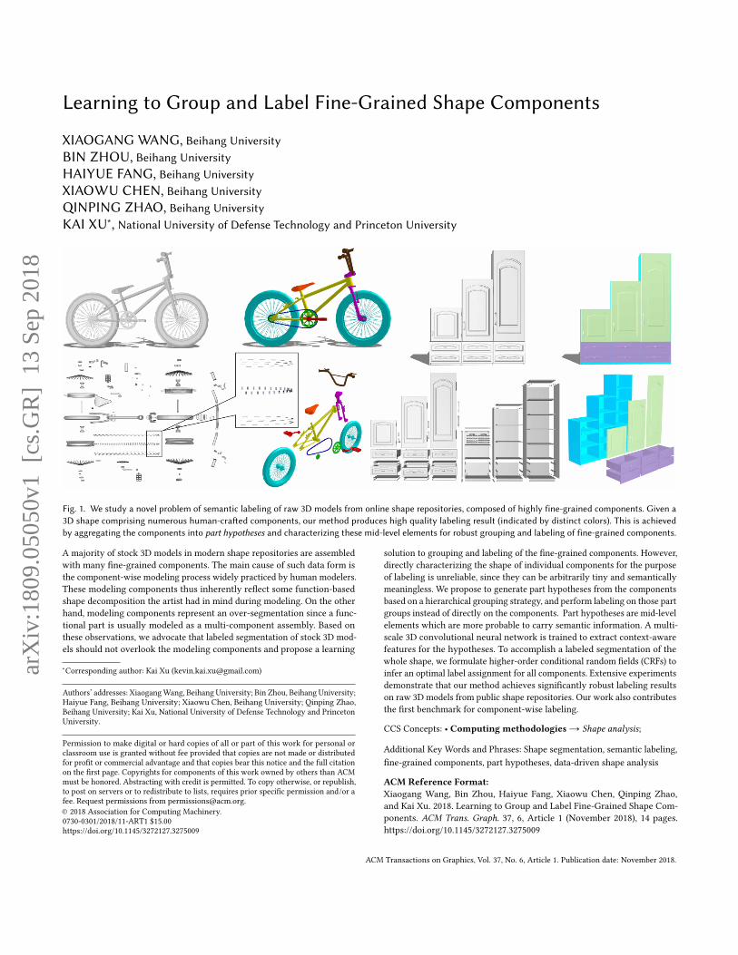
Fig. 1. We study a novel problem of semantic labeling of raw 3D models from online shape repositories, composed of highly fine-grained components. Given a3D shape comprising numerous human-crafted components, our method produces high quality labeling result (indicated by distinct colors). This is achievedby aggregating the components into part hypotheses and characterizing these mid-level elements for robust grouping and labeling of fine-grained components.

A majority of stock 3D models in modern shape repositories are assembledwith many fine-grained components. The main cause of such data form isthe component-wise modeling process widely practiced by human modelers.These modeling components thus inherently reflect some function-basedshape decomposition the artist had in mind during modeling. On the otherhand, modeling components represent an over-segmentation since a func-tional part is usually modeled as a multi-component assembly. Based onthese observations, we advocate that labeled segmentation of stock 3D mod-els should not overlook the modeling components and propose a learning

∗Corresponding author: Kai Xu ([email protected])

Authors’ addresses: XiaogangWang, Beihang University; Bin Zhou, Beihang University;Haiyue Fang, Beihang University; Xiaowu Chen, Beihang University; Qinping Zhao,Beihang University; Kai Xu, National University of Defense Technology and PrincetonUniversity.

Permission to make digital or hard copies of all or part of this work for personal orclassroom use is granted without fee provided that copies are not made or distributedfor profit or commercial advantage and that copies bear this notice and the full citationon the first page. Copyrights for components of this work owned by others than ACMmust be honored. Abstracting with credit is permitted. To copy otherwise, or republish,to post on servers or to redistribute to lists, requires prior specific permission and/or afee. Request permissions from [email protected].© 2018 Association for Computing Machinery.0730-0301/2018/11-ART1 $15.00https://doi.org/10.1145/3272127.3275009

solution to grouping and labeling of the fine-grained components. However,directly characterizing the shape of individual components for the purposeof labeling is unreliable, since they can be arbitrarily tiny and semanticallymeaningless. We propose to generate part hypotheses from the componentsbased on a hierarchical grouping strategy, and perform labeling on those partgroups instead of directly on the components. Part hypotheses are mid-levelelements which are more probable to carry semantic information. A multi-scale 3D convolutional neural network is trained to extract context-awarefeatures for the hypotheses. To accomplish a labeled segmentation of thewhole shape, we formulate higher-order conditional random fields (CRFs) toinfer an optimal label assignment for all components. Extensive experimentsdemonstrate that our method achieves significantly robust labeling resultson raw 3D models from public shape repositories. Our work also contributesthe first benchmark for component-wise labeling.

CCS Concepts: • Computing methodologies→ Shape analysis;

Additional Key Words and Phrases: Shape segmentation, semantic labeling,fine-grained components, part hypotheses, data-driven shape analysis

ACM Reference Format:Xiaogang Wang, Bin Zhou, Haiyue Fang, Xiaowu Chen, Qinping Zhao,and Kai Xu. 2018. Learning to Group and Label Fine-Grained Shape Com-ponents. ACM Trans. Graph. 37, 6, Article 1 (November 2018), 14 pages.https://doi.org/10.1145/3272127.3275009

ACM Transactions on Graphics, Vol. 37, No. 6, Article 1. Publication date: November 2018.

arX

iv:1

809.

0505

0v1

[cs

.GR

] 1

3 Se

p 20

18

https://doi.org/10.1145/3272127.3275009

https://doi.org/10.1145/3272127.3275009

1:2 • Xiaogang Wang, Bin Zhou, Haiyue Fang, Xiaowu Chen, Qinping Zhao, and Kai Xu

># Components

Fig. 2. Statistics on component count (left) and size (right) of the models inShapeNetCore. The left histogram is measured only for car models. In theright one, size is measured by the ratio of bounding box volume between acomponent and the whole shape.

1 INTRODUCTIONSemantic or labeled segmentation of 3D shapes has gained signifi-cant performance boost over recent years, benefiting from the ad-vances of machine learning techniques [Hu et al. 2012; Kalogerakiset al. 2010], and more recently of deep neural networks [Kalogerakiset al. 2017; Su et al. 2017]. Existing methods have so far been dealingwith manifold meshes, point clouds, or volumes. They are, however,not specifically designed to handle most stock 3Dmodels, which typ-ically assembles up to hundreds of highly fine-grained components(Figure 1). Multi-component assembly is the most commonly seendata form in modern 3D shape repositories (e.g., Trimble 3D Ware-house [Tri 2017] and ShapeNet [Chang et al. 2015]). See Figure 2(left)for the statistics of component counts in ShapeNetCore.

Multi-view projective segmentation [Kalogerakis et al. 2017;Wanget al. 2013] is perhaps the most feasible approach for handling multi-component shapes, among all existing techniques. View-based meth-ods are representation independent, making them applicable to non-manifold models. However, a major drawback of this approach isthat it cannot handle shapes with severe self-occlusion. Componentshidden from the surface are invisible to any view, thus cannot belabeled. Figure 3(a) shows such an example: The seats in the car arecompletely occluded by the car shell and thus cannot be segmentedor labeled correctly by view-based methods.

Most off-the-shelf 3D models are created by human modelers ina component-by-component fashion. Generally, human modelerstend to have in mind a meaningful decomposition of the targetobject before starting. Such decomposition is inherently related tofunctionality, mimicking the actual production of the man-madeobjects, e.g., a car is decomposed into shell, hood, wheels, seats, etc.Therefore, we advocate that the segmentation of such models shouldnot overlook the components coming with the models. Meanwhile,these components usually represent an over-segmentation – a func-tional part might be modeled as an assembly of multiple sub-parts.A natural solution to semantic segmentation thus seems to be alabeled grouping of the modeling components.A few facts about the components of stock models, however,

make their grouping and labeling especially difficult. First, the de-composition of these models is often highly fine-grained. See thetiny components the bicycle model in Figure 1 contains. Taking thecar models in ShapeNetCore for example, about 85% contains over100 components. Second, the size of components varies significantly;see Figure 2(right). Third, different modelers may have differentopinions about shape composition, making the components of the

Fig. 3. Hidden components, e.g., car seats in (a), and various fine-graineddecompositions of vehicle wheels (b) found in the ShapeNet.

same functional part highly inconsistent across different shapes.The example in Figure 3(b) shows that the wheel parts from differ-ent vehicle models have very different composition. Due to thesereasons, it is very unreliable to directly characterize the shape ofindividual components for the purpose of labeling.

These facts motivate us to consider larger and more meaningfulelements, for achieving a robust semantic labeling of fine-grainedcomponents. In particular, we propose to generate part hypothesesfrom the components, representing potential functional or semanticparts of the object. This is achieved by a series of effective groupingstrategies, which is proven robust with extensive evaluation. Ourtask then becomes labeling the true part hypotheses while pruningthose false ones, instead of directly labeling the individual com-ponents. Working with part hypotheses enables us to learn moreinformative shape representation, based on which reliable labelingcan be conducted. Part hypothesis is similar in spirit to mid-levelpatch for image understanding which admits more discriminativedescriptors than feature points [Singh et al. 2012].To achieve a powerful part hypotheses labeling, we adopt 3D

Convolutional Neural Networks (CNN) to extract features fromthe volumetric representation of part hypotheses. In order to learnfeatures that capture not only local part geometry but also global,contextual information, we design a network that takes two scalesof 3D volume as input. The local scale encodes the part hypothesisof interest itself, through feature extraction over the voxelizationof the part within its bounding box. The global volume takes thebounding box of the whole shape as input, and encodes the contextwith two channels contrasting the volume occupancy of the parthypothesis itself and that of the remaining parts. The network out-puts the labeling probabilities of the part hypothesis over differentpart categories, which are used for final labeled segmentation.To accomplish a labeled segmentation of the whole shape, we

formulate higher-order Conditional Random Fields (CRFs) to inferan optimal label assignment for each component. Our CRF-basedmodel achieves highly accurate labeling, while saving the effort onpreparing large amount of high-order relational data for training


Learning to Group and Label Fine-Grained Shape Components • 1:3

a deep model. Consequently, our design choice, combining CNN-based part hypothesis feature and higher-order CRFs, achieves agood balance between model generality and complexity.

We validate our approach on ourmulti-component labeling (MCL)benchmark dataset. The multi-component 3D models are collectedfrom both ShapeNet and 3D Warehouse, with all components man-ually labeled. Our method achieves significantly higher accuracyin grouping and labeling highly fine-grained components than al-ternative approaches. We also demonstrate how our method can beapplied to fine-grained part correspondence for 3D shapes, achiev-ing state-of-the-art results.The main contributions of our paper include:

• We study a new problem of labeled segmentation of stock3D models based on the pre-existing, highly fine-grainedcomponents, and approach the problem with a novel solutionof part hypothesis generation and characterization.

• We propose a multi-scale 3D CNN for encoding both localand contextual information for part hypothesis labeling, aswell as a CRF-based formulation for component labeling.

• We build the first benchmark for multi-component labelingwith component-wise ground-truth labels and conduct exten-sive evaluation over the benchmark.

2 RELATED WORKShape segmentation and labeling is one of the most classical andlong-standing problems in shape analysis, with numerous methodshaving been proposed. Early studies [Au et al. 2012; Huang et al.2009; Katz and Tal 2003; Shapira et al. 2010; Zhang et al. 2012] mostutilize hand-crafted geometry features. One geometric feature usu-ally captures very limited aspects about shape decomposition and awider practiced approach is to combine multiple features [Kaloger-akis et al. 2010].To tackle the limitation of hand-crafted features, data-driven

feature learning methods are proposed [Xu et al. 2016]. Guo etal. [2015] learned a compact representation of triangle for 3D meshlabeling by non-linearly combining and hierarchically compressingvarious geometry features with the deep CNNs. Xie et al. [2014]proposed a fast method for 3D mesh segmentation and labelingbased on Extreme Learning Machine. Yi et al. [2017b] proposed amethod, named SyncSpecCNN, to label the semantic part of 3Dmesh.SyncSpecCNN trains vertex functions using CNNS, and conductsspectral analysis to enable kernel weight sharing by using localizedinformation of mesh graphs. These methods achieve promisingperformance, while largely focusing on manifold and/or watertightsurface mesh, but not suited for raw 3D models from modern shaperepositories.Recently, Kalogerakis et al. [2017] proposed a deep architecture

for segmenting and labeling semantic parts of 3D shape by com-bining multi-view fully convolutional networks and surface-basedCRFs. Projection-based methods [Kalogerakis et al. 2017; Wang et al.2013] are suitable for imperfect (e.g., incomplete, self-intersecting,and noisy) 3D shapes, but inherently have a hard time on shapeswith severe self-occlusion. Su et al. [2017] designed a novel type of

neural network, named PointNet, for directly segmenting and label-ing 3D point clouds while respecting the permutation invariance,obtaining state-of-the-art performance on point data.Several unsupervised or semi-supervised methods are proposed

for the co-segmentation and/or co-labeling of a collection of 3Dshapes belonging to the same category [Hu et al. 2012; Huang et al.2011; Lv et al. 2012; Sidi et al. 2011; van Kaick et al. 2013; Wanget al. 2012; Xu et al. 2010]. Most of these methods are based on anover-segmentations of the input shapes. A grouping process is thenconducted to form semantic segmentation and labeling. Such initialover-segments (e.g., superfaces) are analogy to our ‘part hypotheses’.However, they are still too low level to capture meaningful partinformation. Our method benefits from the pre-existing fine-grainedcomponents, which makes part hypothesis based analysis possible.

Fewworks studied on semantic segmentation of multi-componentmodels. Liu et al. [2014] proposed to label and organize 3D scenesobtained from the Trimble 3D Warehouse into consistent hierar-chies capturing semantic and functional substructures. The labelingis based on over-segmentation of the 3D input, and guided by alearned probabilistic grammar. Yi et al. [2017a] proposed a methodof converting the scene-graph of a multi-component shape intosegmented parts by learning a category-specific canonical part hi-erarchy. Their method achieves fine-grained component labeling,while scene graphs are not always available.

3 METHODPlease refer to Figure 4 for an overview of our algorithm pipeline.In the next, we describe the three algorithmic components, includ-ing part hypothesis generation, part hypothesis classification andscoring, and part composition inference and component labeling.

3.1 Generating part hypothesisPart hypothesis. In our work, a semantic part, or part for short,

refers to a semantically independent or functionally complete groupof components. A part hypothesis is a component group which po-tentially represents a semantic part. When searching for a part hy-pothesis, we follow two principles. Firstly, a part hypothesis shouldcover as many as possible components of the corresponding ground-truth part. Secondly, the component coverage of a part hypothesisshould be conservative, meaning that a hypothesis with missingcomponents is preferred over that encompassing components acrossdifferent semantic parts.

Grouping strategy. It is a non-trivial task to generate part hy-potheses meeting the above requirements exactly. It is very likelythat there is not a single optimal criterion that can be applied togenerate hypotheses for any semantic part from a set of compo-nents. For example, the many components of a car wheel can seem-ingly grouped based on a compactness criterion. For bicycle chain,however, the tiny chain links are not compactly stacked at all, forwhich size based grouping might be more appropriate. Therefore,we design a grouping strategy encompassing three heuristic criteria,which are intuitively interpretable and computationally efficient.The grouping for each criterion is performed in a bottom-up fash-ion, based on a nested hierarchy. After that, a hypotheses selection



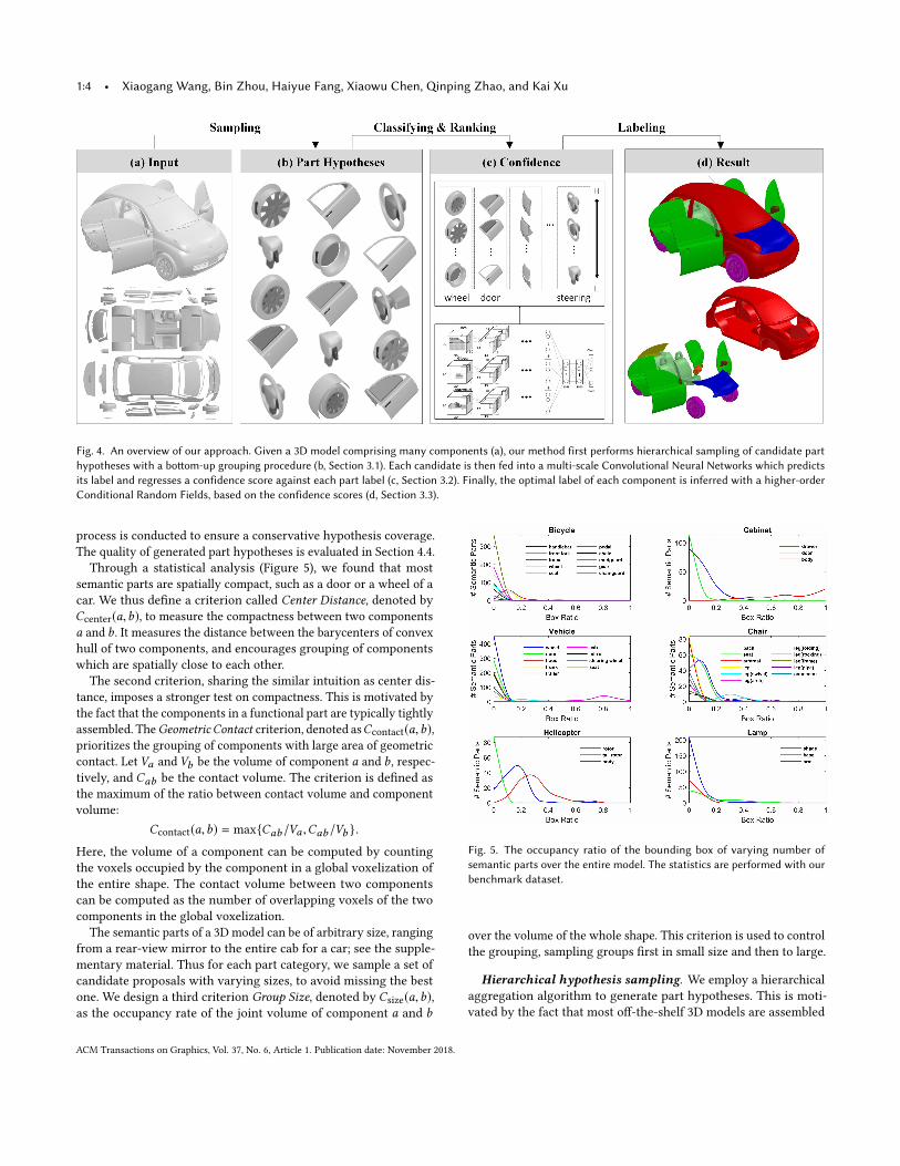
Fig. 4. An overview of our approach. Given a 3D model comprising many components (a), our method first performs hierarchical sampling of candidate parthypotheses with a bottom-up grouping procedure (b, Section 3.1). Each candidate is then fed into a multi-scale Convolutional Neural Networks which predictsits label and regresses a confidence score against each part label (c, Section 3.2). Finally, the optimal label of each component is inferred with a higher-orderConditional Random Fields, based on the confidence scores (d, Section 3.3).

process is conducted to ensure a conservative hypothesis coverage.The quality of generated part hypotheses is evaluated in Section 4.4.

Through a statistical analysis (Figure 5), we found that mostsemantic parts are spatially compact, such as a door or a wheel of acar. We thus define a criterion called Center Distance, denoted byCcenter(a,b), to measure the compactness between two componentsa and b. It measures the distance between the barycenters of convexhull of two components, and encourages grouping of componentswhich are spatially close to each other.

The second criterion, sharing the similar intuition as center dis-tance, imposes a stronger test on compactness. This is motivated bythe fact that the components in a functional part are typically tightlyassembled. TheGeometric Contact criterion, denoted asCcontact(a,b),prioritizes the grouping of components with large area of geometriccontact. Let Va and Vb be the volume of component a and b, respec-tively, and Cab be the contact volume. The criterion is defined asthe maximum of the ratio between contact volume and componentvolume:

Ccontact(a,b) = max{Cab/Va ,Cab/Vb }.Here, the volume of a component can be computed by countingthe voxels occupied by the component in a global voxelization ofthe entire shape. The contact volume between two componentscan be computed as the number of overlapping voxels of the twocomponents in the global voxelization.

The semantic parts of a 3D model can be of arbitrary size, rangingfrom a rear-view mirror to the entire cab for a car; see the supple-mentary material. Thus for each part category, we sample a set ofcandidate proposals with varying sizes, to avoid missing the bestone. We design a third criterion Group Size, denoted by Csize(a,b),as the occupancy rate of the joint volume of component a and b

Fig. 5. The occupancy ratio of the bounding box of varying number ofsemantic parts over the entire model. The statistics are performed with ourbenchmark dataset.

over the volume of the whole shape. This criterion is used to controlthe grouping, sampling groups first in small size and then to large.

Hierarchical hypothesis sampling. We employ a hierarchicalaggregation algorithm to generate part hypotheses. This is moti-vated by the fact that most off-the-shelf 3D models are assembled



Fig. 6. Hierarchical sampling of part hypotheses based on the three group-ing criteria, center distance (a), group size (b) and geometric contact (c),respectively.

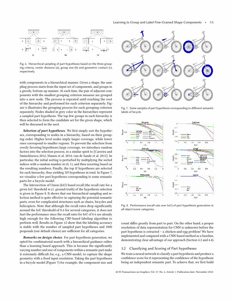
with components in a hierarchical manner. Given a shape, the sam-pling process starts from the input set of components, and groups ina greedy, bottom-up manner. At each time, the pair of adjacent com-ponents with the smallest grouping criterion measure are groupedinto a new node. The process is repeated until reaching the rootof the hierarchy and performed for each criterion separately. Fig-ure 6 illustrates the grouping process for each grouping criterionseparately. Nodes shaded in grey color in the hierarchies representa sampled part hypothesis. The top few groups in each hierarchy isthen selected to form the candidate set for the given shape, whichwill be discussed in the next.

Selection of part hypotheses. We first simply sort the hypothe-ses, corresponding to nodes in a hierarchy, based on their group-ing order. Higher level nodes imply larger coverage, while lowerones correspond to smaller regions. To prevent the selection fromoverly favoring hypotheses large coverage, we introduce randomfactors into the selection process, in a similar spirit to [Carreira andSminchisescu 2012; Manen et al. 2014; van de Sande et al. 2011]. Inparticular, the initial sorting is perturbed by multiplying the sortedindices with a random number in (0, 1), and then resorting based onthe resulting numbers. Finally, the top H hypotheses are selectedfor each hierarchy, thus yielding 3H hypotheses in total. In Figure 7,we visualize a few part hypotheses corresponding to some semanticparts for a bicycle model.

The Intersection of Union (IoU) based recall (the recall rate for agiven IoU threshold w.r.t. ground-truth) of the hypothesis selectionis given in Figure 8. It shows that our hierarchical sampling and se-lection method is quite effective in capturing the potential semanticparts, even for complicated structures such as chairs, bicycles andhelicopters. Note that although the recall rates drop significantlyaround the IoU threshold of 0.6 for several categories, it does nothurt the performance since the recall rates for IoU of 0.6 are alreadyhigh enough for the following CRF-based labeling algorithm toperform well. Results in Figure 12 show that the labeling accuracyis stable with the number of sampled part hypotheses and 1000proposals (our default choice) are sufficient for all categories.

Remarks on design choice. For part hypothesis generation, weopted for combinatorial search with a hierarchical guidance ratherthan a learning based approach. This is because the significantlyvarying number and size of components within a semantic part makeit extremely difficult for, e.g., a CNN model, to capture the shapegeometry with a fixed input resolution. Taking the part hypothesesin a bicycle model (Figure 7) for example, the component size and

Fig. 7. Some samples of part hypothesis corresponding to different semanticlabels of bicycle.

Fig. 8. Performance (recall rate over IoU) of part hypothesis generation inall object/scene categories.

count differ greatly from part to part. On the other hand, a properresolution of data representation for CNN is unknown before thepart hypothesis is extracted – a chicken-and-egg problem! We haveimplemented and compared with a CNN-based method as a baseline,demonstrating clear advantage of our approach (Section 4.2 and 4.4).

3.2 Classifying and Scoring of Part hypothesesWe train a neural network to classify a part hypothesis and produce aconfidence score for it representing the confidence of the hypothesisbeing an independent semantic part. To achieve that, we first build



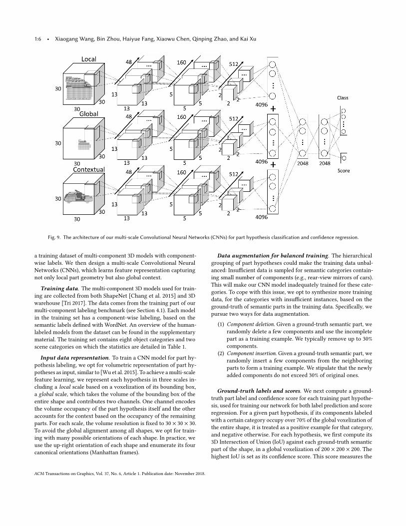
Fig. 9. The architecture of our multi-scale Convolutional Neural Networks (CNNs) for part hypothesis classification and confidence regression.

a training dataset of multi-component 3D models with component-wise labels. We then design a multi-scale Convolutional NeuralNetworks (CNNs), which learns feature representation capturingnot only local part geometry but also global context.

Training data. The multi-component 3D models used for train-ing are collected from both ShapeNet [Chang et al. 2015] and 3Dwarehouse [Tri 2017]. The data comes from the training part of ourmulti-component labeling benchmark (see Section 4.1). Each modelin the training set has a component-wise labeling, based on thesemantic labels defined with WordNet. An overview of the human-labeled models from the dataset can be found in the supplementarymaterial. The training set contains eight object categories and twoscene categories on which the statistics are detailed in Table 1.

Input data representation. To train a CNN model for part hy-pothesis labeling, we opt for volumetric representation of part hy-potheses as input, similar to [Wu et al. 2015]. To achieve amulti-scalefeature learning, we represent each hypothesis in three scales in-cluding a local scale based on a voxelization of its bounding box,a global scale, which takes the volume of the bounding box of theentire shape and contributes two channels. One channel encodesthe volume occupancy of the part hypothesis itself and the otheraccounts for the context based on the occupancy of the remainingparts. For each scale, the volume resolution is fixed to 30 × 30 × 30.To avoid the global alignment among all shapes, we opt for train-ing with many possible orientations of each shape. In practice, weuse the up-right orientation of each shape and enumerate its fourcanonical orientations (Manhattan frames).

Data augmentation for balanced training. The hierarchicalgrouping of part hypotheses could make the training data unbal-anced: Insufficient data is sampled for semantic categories contain-ing small number of components (e.g., rear-view mirrors of cars).This will make our CNN model inadequately trained for these cate-gories. To cope with this issue, we opt to synthesize more trainingdata, for the categories with insufficient instances, based on theground-truth of semantic parts in the training data. Specifically, wepursue two ways for data augmentation.

(1) Component deletion. Given a ground-truth semantic part, werandomly delete a few components and use the incompletepart as a training example. We typically remove up to 30%components.

(2) Component insertion. Given a ground-truth semantic part, werandomly insert a few components from the neighboringparts to form a training example. We stipulate that the newlyadded components do not exceed 30% of original ones.

Ground-truth labels and scores. We next compute a ground-truth part label and confidence score for each training part hypothe-sis, used for training our network for both label prediction and scoreregression. For a given part hypothesis, if its components labeledwith a certain category occupy over 70% of the global voxelization ofthe entire shape, it is treated as a positive example for that category,and negative otherwise. For each hypothesis, we first compute its3D Intersection of Union (IoU) against each ground-truth semanticpart of the shape, in a global voxelization of 200 × 200 × 200. Thehighest IoU is set as its confidence score. This score measures the



confidence of a hypothesis being an independent semantic part,which will be utilized in the final label inference in Section 3.3.

Network architecture. We design a multi-scale ConvolutionalNeural Networks (CNNs). The architecture of our network is givenin Figure 9. The network has three towers, taking the inputs cor-responding to the local and the two global channels mentionedabove. We refer to these towers as local, global and contextual, re-spectively; see Figure 9. The feature maps output by the three towersare concatenated into one feature vector, and then fed into a fewfully connected layers, yielding a 2048 feature vector. The final fullyconnected layer predicts a label and regresses a score for the inputpart hypothesis. In particular, our network produces a probabilitydistribution over K + 1 part labels, p = (p0, . . . ,pK ), with label 0being null label. An unrecognized part is assigned with a null label.The second output is confidence score r . We use a joint loss L forboth hypothesis classification and score regression:

L(p, r , c, s) = Lcls(p, c) + Lreg(r , s), (1)

where Lcls(p, c) = − logpc is cross-entropy loss for label c . and Lregis smooth L1 loss.

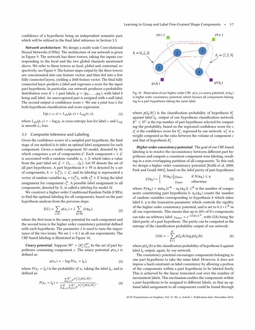
3.3 Composite Inference and LabelingGiven the confidence scores of a sampled part hypothesis, the finalstage of our method is to infer an optimal label assignment for eachcomponent. Given a multi-component 3D model, denoted by M ,which comprises a set of components C. Each component c ∈ Cis associated with a random variable xc ∈ X which takes a valuefrom the part label set L = {l1, . . . , lK }. Let H denote the set ofall part hypotheses. A part hypothesis h ∈ H is denoted by a setof components, h B {chi }i ⊂ C, and its labeling is represented avector of random variables xh = (xhi )i , with xhi ∈ X being the labelassignment for component chi . A possible label assignment to allcomponents, denoted by X , is called a labeling for modelM .We construct a higher-order Conditional Random Fields (CRFs),

to find the optimal labeling for all components, based on the parthypothesis analysis from the previous steps:

E(L) =∑c ∈C

φ(xc ) + λ∑h∈H

ψ (xh ), (2)

where the first term is the unary potential for each component andthe second term is the higher order consistency potential definedwith each hypothesis. The parameter λ is used to tune the impor-tance of the two terms. We set λ = 0.1 in all our experiments. TheCRF-based labeling is illustrated in Figure 10,

Unary potential. Suppose Hc = {hci }H c

i=1 be the set of part hy-potheses containing component c . The unary potential φ(xc ) isdefined as:

φ(xc ) = − log P(xc = lk ), (3)

where P(xc = lk ) is the probability of xc taking the label lk , and isdefined as:

P(xc = lk ) =∑Kc

i=1ewci s

ci p(lk |hci )∑K

k=1∑Kc

j=1ewcj s

cj p(lk |hcj )

, (4)

Fig. 10. Illustration of our higher-order CRF. φ(xi ) is unary potential.ψ (xh )is higher order consistency potential, which favours all components belong-ing to a part hypothesis taking the same label.

where p(lk |hci ) is the classification probability of hypothesis hciagainst label lk , output of our hypothesis classification network.Kc ⩽ Hc is the top number of part hypotheses selected for comput-ing the probability, based on the regressed confidence score for c .sci is the confidence score for hci , regressed by our network.wc

i is aweight computed as the ratio between the volume of component cand that of hypothesis hci .

Higher order consistency potential. The goal of our CRF-basedlabeling is to resolve the inconsistency between different part hy-potheses and compute a consistent component-wise labeling, result-ing in a non-overlapping partition of all components. To this end,we design a higher order consistency potential [Kohli et al. 2008;Park and Gould 2003], based on the label purity of part hypotheses:

ψ (xh ) ={

N (xh ) 1ηγmax, if N (xh ) ≤ η

γmax, otherwise(5)

where N (xh ) = mink {Ch − nk (xh )}. Ch is the number of compo-nents constituting part hypothesis h. nk (xh ) counts the numberof random variables corresponding to hypothesis h which takeslabel k . η is the truncation parameter which controls the rigidityof the higher order consistency potential, and is set to 0.2 ∗Ch inall our experiments. This means that up to 20% of h’s componentscan take an arbitrary label. γmax = e−G(h)/Ch

, with G(h) being thelabel purity of a part hypothesis. The purity can be computed as theentropy of the classification probability output of our network:

G(h) = −K∑k=1

p(lk |h) logp(lk |h). (6)

where p(lk |h) is the classification probability of hypothesis h againstlabel lk output, again, by our network.The consistency potential encourages components belonging to

one part hypothesis to take the same label. However, it does notimpose a hard constraint on label consistency by allowing a portionof the components within a part hypothesis to be labeled freely.This is achieved by the linear truncated cost over the number ofinconsistent labels. This mechanism enables the components withina part hypothesis to be assigned to different labels, so that an op-timal label assignment to all components could be found through



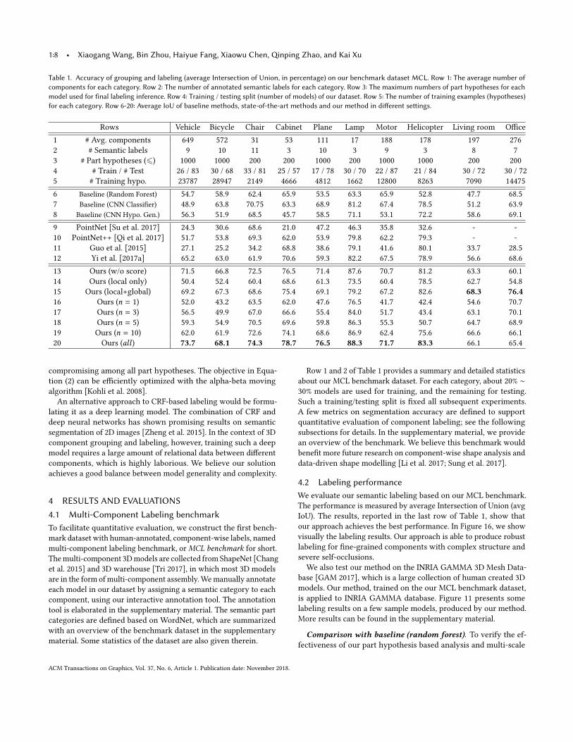
Table 1. Accuracy of grouping and labeling (average Intersection of Union, in percentage) on our benchmark dataset MCL. Row 1: The average number ofcomponents for each category. Row 2: The number of annotated semantic labels for each category. Row 3: The maximum numbers of part hypotheses for eachmodel used for final labeling inference. Row 4: Training / testing split (number of models) of our dataset. Row 5: The number of training examples (hypotheses)for each category. Row 6-20: Average IoU of baseline methods, state-of-the-art methods and our method in different settings.

Rows Vehicle Bicycle Chair Cabinet Plane Lamp Motor Helicopter Living room Office1 # Avg. components 649 572 31 53 111 17 188 178 197 2762 # Semantic labels 9 10 11 3 10 3 9 3 8 73 # Part hypotheses (⩽) 1000 1000 200 200 1000 200 1000 1000 200 2004 # Train / # Test 26 / 83 30 / 68 33 / 81 25 / 57 17 / 78 30 / 70 22 / 87 21 / 84 30 / 72 30 / 725 # Training hypo. 23787 28947 2149 4666 4812 1662 12800 8263 7090 144756 Baseline (Random Forest) 54.7 58.9 62.4 65.9 53.5 63.3 65.9 52.8 47.7 68.57 Baseline (CNN Classifier) 48.9 63.8 70.75 63.3 68.9 81.2 67.4 78.5 51.2 63.98 Baseline (CNN Hypo. Gen.) 56.3 51.9 68.5 45.7 58.5 71.1 53.1 72.2 58.6 69.19 PointNet [Su et al. 2017] 24.3 30.6 68.6 21.0 47.2 46.3 35.8 32.6 - -10 PointNet++ [Qi et al. 2017] 51.7 53.8 69.3 62.0 53.9 79.8 62.2 79.3 - -11 Guo et al. [2015] 27.1 25.2 34.2 68.8 38.6 79.1 41.6 80.1 33.7 28.512 Yi et al. [2017a] 65.2 63.0 61.9 70.6 59.3 82.2 67.5 78.9 56.6 68.613 Ours (w/o score) 71.5 66.8 72.5 76.5 71.4 87.6 70.7 81.2 63.3 60.114 Ours (local only) 50.4 52.4 60.4 68.6 61.3 73.5 60.4 78.5 62.7 54.815 Ours (local+global) 69.2 67.3 68.6 75.4 69.1 79.2 67.2 82.6 68.3 76.416 Ours (n = 1) 52.0 43.2 63.5 62.0 47.6 76.5 41.7 42.4 54.6 70.717 Ours (n = 3) 56.5 49.9 67.0 66.6 55.4 84.0 51.7 43.4 63.1 70.118 Ours (n = 5) 59.3 54.9 70.5 69.6 59.8 86.3 55.3 50.7 64.7 68.919 Ours (n = 10) 62.0 61.9 72.6 74.1 68.6 86.9 62.4 75.6 66.6 66.120 Ours (all ) 73.7 68.1 74.3 78.7 76.5 88.3 71.7 83.3 66.1 65.4

compromising among all part hypotheses. The objective in Equa-tion (2) can be efficiently optimized with the alpha-beta movingalgorithm [Kohli et al. 2008].An alternative approach to CRF-based labeling would be formu-

lating it as a deep learning model. The combination of CRF anddeep neural networks has shown promising results on semanticsegmentation of 2D images [Zheng et al. 2015]. In the context of 3Dcomponent grouping and labeling, however, training such a deepmodel requires a large amount of relational data between differentcomponents, which is highly laborious. We believe our solutionachieves a good balance between model generality and complexity.

4 RESULTS AND EVALUATIONS

4.1 Multi-Component Labeling benchmarkTo facilitate quantitative evaluation, we construct the first bench-mark dataset with human-annotated, component-wise labels, namedmulti-component labeling benchmark, orMCL benchmark for short.Themulti-component 3Dmodels are collected from ShapeNet [Changet al. 2015] and 3D warehouse [Tri 2017], in which most 3D modelsare in the form of multi-component assembly.Wemanually annotateeach model in our dataset by assigning a semantic category to eachcomponent, using our interactive annotation tool. The annotationtool is elaborated in the supplementary material. The semantic partcategories are defined based on WordNet, which are summarizedwith an overview of the benchmark dataset in the supplementarymaterial. Some statistics of the dataset are also given therein.

Row 1 and 2 of Table 1 provides a summary and detailed statisticsabout our MCL benchmark dataset. For each category, about 20% ∼30% models are used for training, and the remaining for testing.Such a training/testing split is fixed all subsequent experiments.A few metrics on segmentation accuracy are defined to supportquantitative evaluation of component labeling; see the followingsubsections for details. In the supplementary material, we providean overview of the benchmark. We believe this benchmark wouldbenefit more future research on component-wise shape analysis anddata-driven shape modelling [Li et al. 2017; Sung et al. 2017].

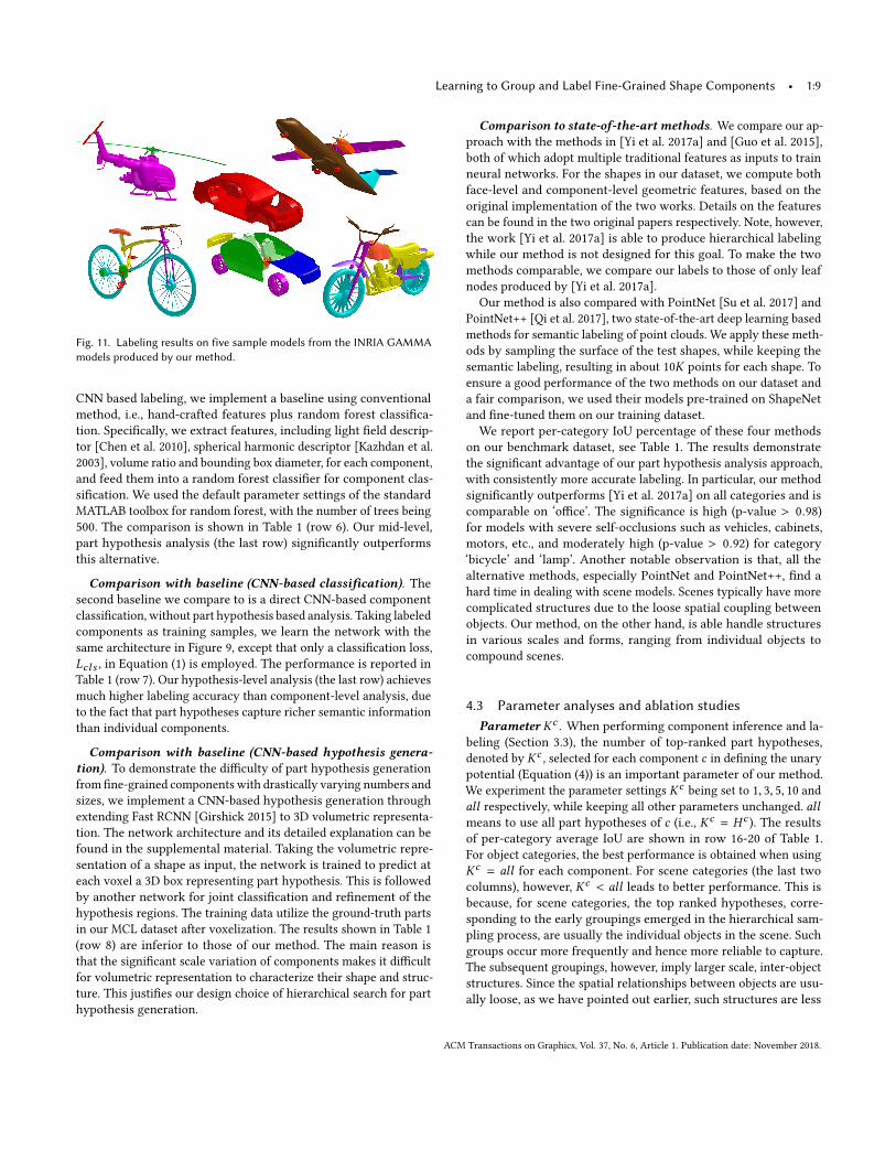
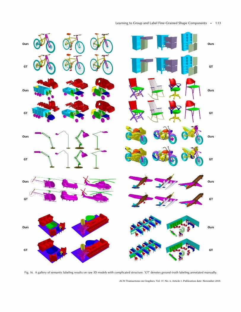
4.2 Labeling performanceWe evaluate our semantic labeling based on our MCL benchmark.The performance is measured by average Intersection of Union (avgIoU). The results, reported in the last row of Table 1, show thatour approach achieves the best performance. In Figure 16, we showvisually the labeling results. Our approach is able to produce robustlabeling for fine-grained components with complex structure andsevere self-occlusions.We also test our method on the INRIA GAMMA 3D Mesh Data-

base [GAM 2017], which is a large collection of human created 3Dmodels. Our method, trained on the our MCL benchmark dataset,is applied to INRIA GAMMA database. Figure 11 presents somelabeling results on a few sample models, produced by our method.More results can be found in the supplementary material.

Comparison with baseline (random forest). To verify the ef-fectiveness of our part hypothesis based analysis and multi-scale



Fig. 11. Labeling results on five sample models from the INRIA GAMMAmodels produced by our method.

CNN based labeling, we implement a baseline using conventionalmethod, i.e., hand-crafted features plus random forest classifica-tion. Specifically, we extract features, including light field descrip-tor [Chen et al. 2010], spherical harmonic descriptor [Kazhdan et al.2003], volume ratio and bounding box diameter, for each component,and feed them into a random forest classifier for component clas-sification. We used the default parameter settings of the standardMATLAB toolbox for random forest, with the number of trees being500. The comparison is shown in Table 1 (row 6). Our mid-level,part hypothesis analysis (the last row) significantly outperformsthis alternative.

Comparison with baseline (CNN-based classification). Thesecond baseline we compare to is a direct CNN-based componentclassification, without part hypothesis based analysis. Taking labeledcomponents as training samples, we learn the network with thesame architecture in Figure 9, except that only a classification loss,Lcls , in Equation (1) is employed. The performance is reported inTable 1 (row 7). Our hypothesis-level analysis (the last row) achievesmuch higher labeling accuracy than component-level analysis, dueto the fact that part hypotheses capture richer semantic informationthan individual components.

Comparison with baseline (CNN-based hypothesis genera-tion). To demonstrate the difficulty of part hypothesis generationfrom fine-grained components with drastically varying numbers andsizes, we implement a CNN-based hypothesis generation throughextending Fast RCNN [Girshick 2015] to 3D volumetric representa-tion. The network architecture and its detailed explanation can befound in the supplemental material. Taking the volumetric repre-sentation of a shape as input, the network is trained to predict ateach voxel a 3D box representing part hypothesis. This is followedby another network for joint classification and refinement of thehypothesis regions. The training data utilize the ground-truth partsin our MCL dataset after voxelization. The results shown in Table 1(row 8) are inferior to those of our method. The main reason isthat the significant scale variation of components makes it difficultfor volumetric representation to characterize their shape and struc-ture. This justifies our design choice of hierarchical search for parthypothesis generation.

Comparison to state-of-the-art methods. We compare our ap-proach with the methods in [Yi et al. 2017a] and [Guo et al. 2015],both of which adopt multiple traditional features as inputs to trainneural networks. For the shapes in our dataset, we compute bothface-level and component-level geometric features, based on theoriginal implementation of the two works. Details on the featurescan be found in the two original papers respectively. Note, however,the work [Yi et al. 2017a] is able to produce hierarchical labelingwhile our method is not designed for this goal. To make the twomethods comparable, we compare our labels to those of only leafnodes produced by [Yi et al. 2017a].

Our method is also compared with PointNet [Su et al. 2017] andPointNet++ [Qi et al. 2017], two state-of-the-art deep learning basedmethods for semantic labeling of point clouds. We apply these meth-ods by sampling the surface of the test shapes, while keeping thesemantic labeling, resulting in about 10K points for each shape. Toensure a good performance of the two methods on our dataset anda fair comparison, we used their models pre-trained on ShapeNetand fine-tuned them on our training dataset.We report per-category IoU percentage of these four methods

on our benchmark dataset, see Table 1. The results demonstratethe significant advantage of our part hypothesis analysis approach,with consistently more accurate labeling. In particular, our methodsignificantly outperforms [Yi et al. 2017a] on all categories and iscomparable on ‘office’. The significance is high (p-value > 0.98)for models with severe self-occlusions such as vehicles, cabinets,motors, etc., and moderately high (p-value > 0.92) for category‘bicycle’ and ‘lamp’. Another notable observation is that, all thealternative methods, especially PointNet and PointNet++, find ahard time in dealing with scene models. Scenes typically have morecomplicated structures due to the loose spatial coupling betweenobjects. Our method, on the other hand, is able handle structuresin various scales and forms, ranging from individual objects tocompound scenes.

4.3 Parameter analyses and ablation studiesParameter Kc . When performing component inference and la-

beling (Section 3.3), the number of top-ranked part hypotheses,denoted by Kc , selected for each component c in defining the unarypotential (Equation (4)) is an important parameter of our method.We experiment the parameter settings Kc being set to 1, 3, 5, 10 andall respectively, while keeping all other parameters unchanged. allmeans to use all part hypotheses of c (i.e., Kc = Hc ). The resultsof per-category average IoU are shown in row 16-20 of Table 1.For object categories, the best performance is obtained when usingKc = all for each component. For scene categories (the last twocolumns), however, Kc < all leads to better performance. This isbecause, for scene categories, the top ranked hypotheses, corre-sponding to the early groupings emerged in the hierarchical sam-pling process, are usually the individual objects in the scene. Suchgroups occur more frequently and hence more reliable to capture.The subsequent groupings, however, imply larger scale, inter-objectstructures. Since the spatial relationships between objects are usu-ally loose, as we have pointed out earlier, such structures are less



Fig. 12. Labeling accuracy (average IoU) vs. number of part hypotheses.

reliable (hard to learn), especially when the grouping scale becomesvery large.

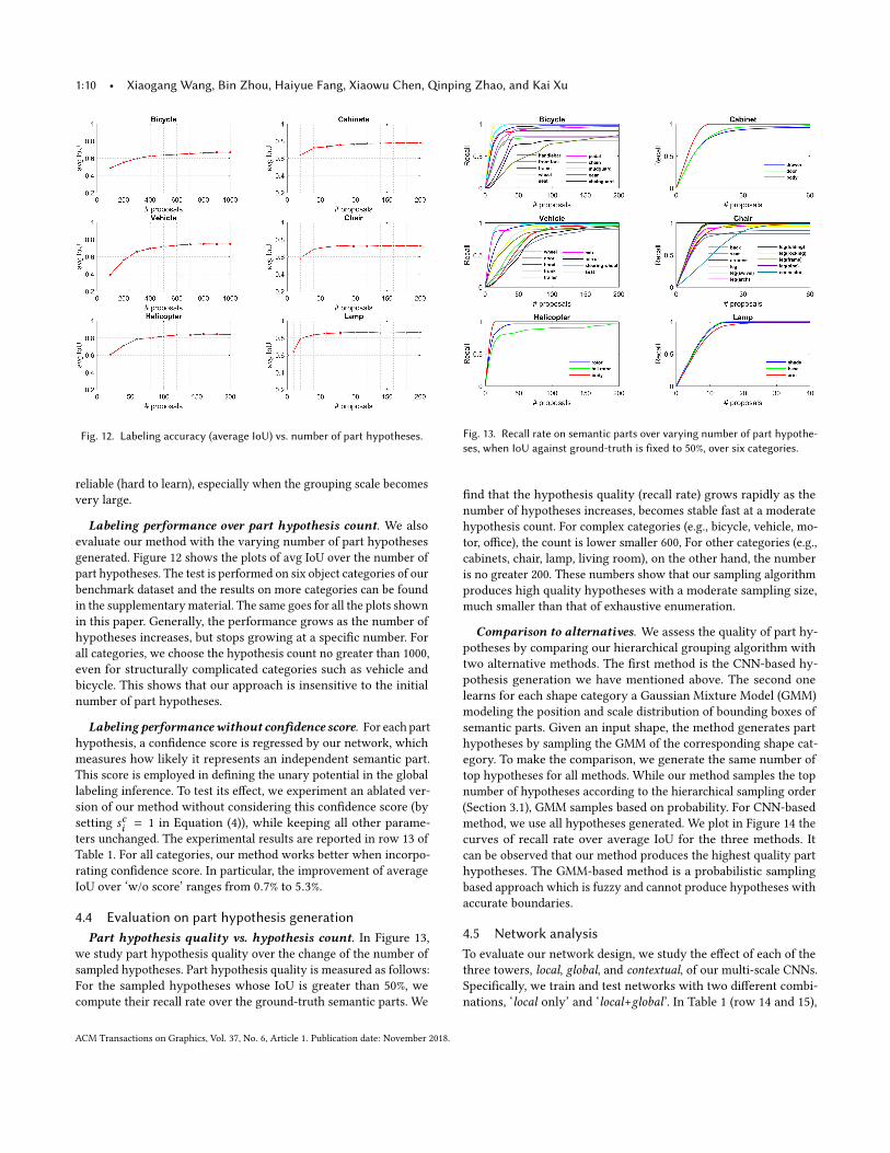
Labeling performance over part hypothesis count. We alsoevaluate our method with the varying number of part hypothesesgenerated. Figure 12 shows the plots of avg IoU over the number ofpart hypotheses. The test is performed on six object categories of ourbenchmark dataset and the results on more categories can be foundin the supplementarymaterial. The same goes for all the plots shownin this paper. Generally, the performance grows as the number ofhypotheses increases, but stops growing at a specific number. Forall categories, we choose the hypothesis count no greater than 1000,even for structurally complicated categories such as vehicle andbicycle. This shows that our approach is insensitive to the initialnumber of part hypotheses.

Labeling performancewithout confidence score. For each parthypothesis, a confidence score is regressed by our network, whichmeasures how likely it represents an independent semantic part.This score is employed in defining the unary potential in the globallabeling inference. To test its effect, we experiment an ablated ver-sion of our method without considering this confidence score (bysetting sci = 1 in Equation (4)), while keeping all other parame-ters unchanged. The experimental results are reported in row 13 ofTable 1. For all categories, our method works better when incorpo-rating confidence score. In particular, the improvement of averageIoU over ‘w/o score’ ranges from 0.7% to 5.3%.

4.4 Evaluation on part hypothesis generationPart hypothesis quality vs. hypothesis count. In Figure 13,

we study part hypothesis quality over the change of the number ofsampled hypotheses. Part hypothesis quality is measured as follows:For the sampled hypotheses whose IoU is greater than 50%, wecompute their recall rate over the ground-truth semantic parts. We

Fig. 13. Recall rate on semantic parts over varying number of part hypothe-ses, when IoU against ground-truth is fixed to 50%, over six categories.

find that the hypothesis quality (recall rate) grows rapidly as thenumber of hypotheses increases, becomes stable fast at a moderatehypothesis count. For complex categories (e.g., bicycle, vehicle, mo-tor, office), the count is lower smaller 600, For other categories (e.g.,cabinets, chair, lamp, living room), on the other hand, the numberis no greater 200. These numbers show that our sampling algorithmproduces high quality hypotheses with a moderate sampling size,much smaller than that of exhaustive enumeration.

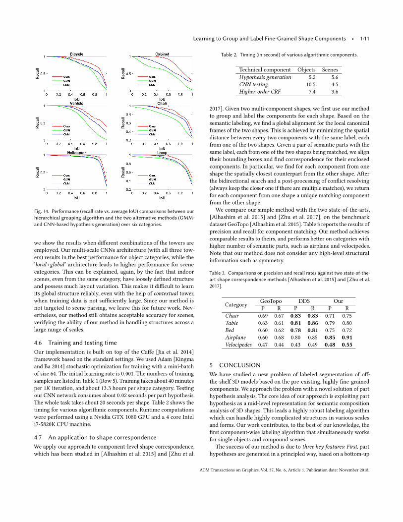
Comparison to alternatives. We assess the quality of part hy-potheses by comparing our hierarchical grouping algorithm withtwo alternative methods. The first method is the CNN-based hy-pothesis generation we have mentioned above. The second onelearns for each shape category a Gaussian Mixture Model (GMM)modeling the position and scale distribution of bounding boxes ofsemantic parts. Given an input shape, the method generates parthypotheses by sampling the GMM of the corresponding shape cat-egory. To make the comparison, we generate the same number oftop hypotheses for all methods. While our method samples the topnumber of hypotheses according to the hierarchical sampling order(Section 3.1), GMM samples based on probability. For CNN-basedmethod, we use all hypotheses generated. We plot in Figure 14 thecurves of recall rate over average IoU for the three methods. Itcan be observed that our method produces the highest quality parthypotheses. The GMM-based method is a probabilistic samplingbased approach which is fuzzy and cannot produce hypotheses withaccurate boundaries.

4.5 Network analysisTo evaluate our network design, we study the effect of each of thethree towers, local, global, and contextual, of our multi-scale CNNs.Specifically, we train and test networks with two different combi-nations, ‘local only’ and ‘local+global’. In Table 1 (row 14 and 15),



Fig. 14. Performance (recall rate vs. average IoU) comparisons between ourhierarchical grouping algorithm and the two alternative methods (GMM-and CNN-based hypothesis generation) over six categories.

we show the results when different combinations of the towers areemployed. Our multi-scale CNNs architecture (with all three tow-ers) results in the best performance for object categories, while the‘local+global’ architecture leads to higher performance for scenecategories. This can be explained, again, by the fact that indoorscenes, even from the same category, have loosely defined structureand possess much layout variation. This makes it difficult to learnits global structure reliably, even with the help of contextual tower,when training data is not sufficiently large. Since our method isnot targeted to scene parsing, we leave this for future work. Nev-ertheless, our method still obtains acceptable accuracy for scenes,verifying the ability of our method in handling structures across alarge range of scales.

4.6 Training and testing timeOur implementation is built on top of the Caffe [Jia et al. 2014]framework based on the standard settings. We used Adam [Kingmaand Ba 2014] stochastic optimization for training with a mini-batchof size 64. The initial learning rate is 0.001. The numbers of trainingsamples are listed in Table 1 (Row 5). Training takes about 40minutesper 1K iteration, and about 13.3 hours per shape category. Testingour CNN network consumes about 0.02 seconds per part hypothesis.The whole task takes about 20 seconds per shape. Table 2 shows thetiming for various algorithmic components. Runtime computationswere performed using a Nvidia GTX 1080 GPU and a 4 core Inteli7-5820K CPU machine.

4.7 An application to shape correspondenceWe apply our approach to component-level shape correspondence,which has been studied in [Alhashim et al. 2015] and [Zhu et al.

Table 2. Timing (in second) of various algorithmic components.

Technical component Objects ScenesHypothesis generation 5.2 5.6CNN testing 10.5 4.5Higher-order CRF 7.4 3.6

2017]. Given two multi-component shapes, we first use our methodto group and label the components for each shape. Based on thesemantic labeling, we find a global alignment for the local canonicalframes of the two shapes. This is achieved by minimizing the spatialdistance between every two components with the same label, eachfrom one of the two shapes. Given a pair of semantic parts with thesame label, each from one of the two shapes being matched, we aligntheir bounding boxes and find correspondence for their enclosedcomponents. In particular, we find for each component from oneshape the spatially closest counterpart from the other shape. Afterthe bidirectional search and a post-processing of conflict resolving(always keep the closer one if there are multiple matches), we returnfor each component from one shape a unique matching componentfrom the other shape.We compare our simple method with the two state-of-the-arts,

[Alhashim et al. 2015] and [Zhu et al. 2017], on the benchmarkdataset GeoTopo [Alhashim et al. 2015]. Table 3 reports the results ofprecision and recall for component matching. Our method achievescomparable results to theirs, and performs better on categories withhigher number of semantic parts, such as airplane and velocipedes.Note that our method does not consider any high-level structuralinformation such as symmetry.

Table 3. Comparisons on precision and recall rates against two state-of-the-art shape correspondence methods [Alhashim et al. 2015] and [Zhu et al.2017].

Category GeoTopo DDS OurP R P R P R

Chair 0.69 0.67 0.83 0.83 0.71 0.75Table 0.63 0.61 0.81 0.86 0.79 0.80Bed 0.60 0.62 0.78 0.81 0.75 0.72Airplane 0.60 0.68 0.80 0.85 0.85 0.91Velocipedes 0.47 0.44 0.43 0.49 0.48 0.55

5 CONCLUSIONWe have studied a new problem of labeled segmentation of off-the-shelf 3D models based on the pre-existing, highly fine-grainedcomponents. We approach the problem with a novel solution of parthypothesis analysis. The core idea of our approach is exploiting parthypothesis as a mid-level representation for semantic compositionanalysis of 3D shapes. This leads a highly robust labeling algorithmwhich can handle highly complicated structures in various scalesand forms. Our work contributes, to the best of our knowledge, thefirst component-wise labeling algorithm that simultaneously worksfor single objects and compound scenes.

The success of our method is due to three key features: First, parthypotheses are generated in a principled way, based on a bottom-up



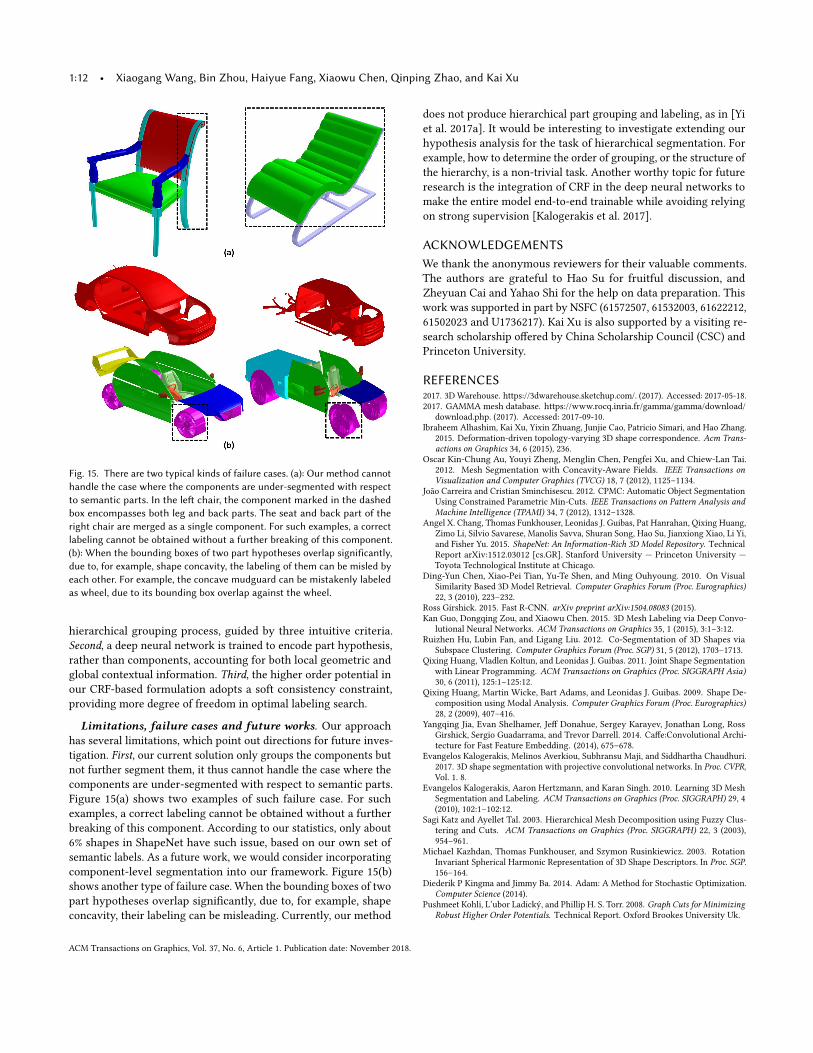
Fig. 15. There are two typical kinds of failure cases. (a): Our method cannothandle the case where the components are under-segmented with respectto semantic parts. In the left chair, the component marked in the dashedbox encompasses both leg and back parts. The seat and back part of theright chair are merged as a single component. For such examples, a correctlabeling cannot be obtained without a further breaking of this component.(b): When the bounding boxes of two part hypotheses overlap significantly,due to, for example, shape concavity, the labeling of them can be misled byeach other. For example, the concave mudguard can be mistakenly labeledas wheel, due to its bounding box overlap against the wheel.

hierarchical grouping process, guided by three intuitive criteria.Second, a deep neural network is trained to encode part hypothesis,rather than components, accounting for both local geometric andglobal contextual information. Third, the higher order potential inour CRF-based formulation adopts a soft consistency constraint,providing more degree of freedom in optimal labeling search.

Limitations, failure cases and future works. Our approachhas several limitations, which point out directions for future inves-tigation. First, our current solution only groups the components butnot further segment them, it thus cannot handle the case where thecomponents are under-segmented with respect to semantic parts.Figure 15(a) shows two examples of such failure case. For suchexamples, a correct labeling cannot be obtained without a furtherbreaking of this component. According to our statistics, only about6% shapes in ShapeNet have such issue, based on our own set ofsemantic labels. As a future work, we would consider incorporatingcomponent-level segmentation into our framework. Figure 15(b)shows another type of failure case. When the bounding boxes of twopart hypotheses overlap significantly, due to, for example, shapeconcavity, their labeling can be misleading. Currently, our method

does not produce hierarchical part grouping and labeling, as in [Yiet al. 2017a]. It would be interesting to investigate extending ourhypothesis analysis for the task of hierarchical segmentation. Forexample, how to determine the order of grouping, or the structure ofthe hierarchy, is a non-trivial task. Another worthy topic for futureresearch is the integration of CRF in the deep neural networks tomake the entire model end-to-end trainable while avoiding relyingon strong supervision [Kalogerakis et al. 2017].

ACKNOWLEDGEMENTSWe thank the anonymous reviewers for their valuable comments.The authors are grateful to Hao Su for fruitful discussion, andZheyuan Cai and Yahao Shi for the help on data preparation. Thiswork was supported in part by NSFC (61572507, 61532003, 61622212,61502023 and U1736217). Kai Xu is also supported by a visiting re-search scholarship offered by China Scholarship Council (CSC) andPrinceton University.

REFERENCES2017. 3DWarehouse. https://3dwarehouse.sketchup.com/. (2017). Accessed: 2017-05-18.2017. GAMMA mesh database. https://www.rocq.inria.fr/gamma/gamma/download/

download.php. (2017). Accessed: 2017-09-10.Ibraheem Alhashim, Kai Xu, Yixin Zhuang, Junjie Cao, Patricio Simari, and Hao Zhang.

2015. Deformation-driven topology-varying 3D shape correspondence. Acm Trans-actions on Graphics 34, 6 (2015), 236.

Oscar Kin-Chung Au, Youyi Zheng, Menglin Chen, Pengfei Xu, and Chiew-Lan Tai.2012. Mesh Segmentation with Concavity-Aware Fields. IEEE Transactions onVisualization and Computer Graphics (TVCG) 18, 7 (2012), 1125–1134.

João Carreira and Cristian Sminchisescu. 2012. CPMC: Automatic Object SegmentationUsing Constrained Parametric Min-Cuts. IEEE Transactions on Pattern Analysis andMachine Intelligence (TPAMI) 34, 7 (2012), 1312–1328.

Angel X. Chang, Thomas Funkhouser, Leonidas J. Guibas, Pat Hanrahan, Qixing Huang,Zimo Li, Silvio Savarese, Manolis Savva, Shuran Song, Hao Su, Jianxiong Xiao, Li Yi,and Fisher Yu. 2015. ShapeNet: An Information-Rich 3D Model Repository. TechnicalReport arXiv:1512.03012 [cs.GR]. Stanford University — Princeton University —Toyota Technological Institute at Chicago.

Ding-Yun Chen, Xiao-Pei Tian, Yu-Te Shen, and Ming Ouhyoung. 2010. On VisualSimilarity Based 3D Model Retrieval. Computer Graphics Forum (Proc. Eurographics)22, 3 (2010), 223–232.

Ross Girshick. 2015. Fast R-CNN. arXiv preprint arXiv:1504.08083 (2015).Kan Guo, Dongqing Zou, and Xiaowu Chen. 2015. 3D Mesh Labeling via Deep Convo-

lutional Neural Networks. ACM Transactions on Graphics 35, 1 (2015), 3:1–3:12.Ruizhen Hu, Lubin Fan, and Ligang Liu. 2012. Co-Segmentation of 3D Shapes via

Subspace Clustering. Computer Graphics Forum (Proc. SGP) 31, 5 (2012), 1703–1713.Qixing Huang, Vladlen Koltun, and Leonidas J. Guibas. 2011. Joint Shape Segmentation

with Linear Programming. ACM Transactions on Graphics (Proc. SIGGRAPH Asia)30, 6 (2011), 125:1–125:12.

Qixing Huang, Martin Wicke, Bart Adams, and Leonidas J. Guibas. 2009. Shape De-composition using Modal Analysis. Computer Graphics Forum (Proc. Eurographics)28, 2 (2009), 407–416.

Yangqing Jia, Evan Shelhamer, Jeff Donahue, Sergey Karayev, Jonathan Long, RossGirshick, Sergio Guadarrama, and Trevor Darrell. 2014. Caffe:Convolutional Archi-tecture for Fast Feature Embedding. (2014), 675–678.

Evangelos Kalogerakis, Melinos Averkiou, Subhransu Maji, and Siddhartha Chaudhuri.2017. 3D shape segmentation with projective convolutional networks. In Proc. CVPR,Vol. 1. 8.

Evangelos Kalogerakis, Aaron Hertzmann, and Karan Singh. 2010. Learning 3D MeshSegmentation and Labeling. ACM Transactions on Graphics (Proc. SIGGRAPH) 29, 4(2010), 102:1–102:12.

Sagi Katz and Ayellet Tal. 2003. Hierarchical Mesh Decomposition using Fuzzy Clus-tering and Cuts. ACM Transactions on Graphics (Proc. SIGGRAPH) 22, 3 (2003),954–961.

Michael Kazhdan, Thomas Funkhouser, and Szymon Rusinkiewicz. 2003. RotationInvariant Spherical Harmonic Representation of 3D Shape Descriptors. In Proc. SGP.156–164.

Diederik P Kingma and Jimmy Ba. 2014. Adam: A Method for Stochastic Optimization.Computer Science (2014).

Pushmeet Kohli, L’ubor Ladický, and Phillip H. S. Torr. 2008. Graph Cuts for MinimizingRobust Higher Order Potentials. Technical Report. Oxford Brookes University Uk.


https://3dwarehouse.sketchup.com/

https://www.rocq.inria.fr/gamma/gamma/download/download.php

https://www.rocq.inria.fr/gamma/gamma/download/download.php


Fig. 16. A gallery of semantic labeling results on raw 3D models with complicated structure. ‘GT’ denotes ground-truth labeling annotated manually.



Jun Li, Kai Xu, Siddhartha Chaudhuri, Ersin Yumer, Hao Zhang, and Leonidas Guibas.2017. GRASS: Generative Recursive Autoencoders for Shape Structures. ACMTransactions on Graphics (Proc. of SIGGRAPH) 36, 4 (2017), 52.

Tianqiang Liu, Siddhartha Chaudhuri, Vladimir G. Kim, Qi-Xing Huang, Niloy J. Mitra,and Thomas Funkhouser. 2014. Creating Consistent Scene Graphs Using a Proba-bilistic Grammar. ACM Transactions on Graphics (Proc. SIGGRAPH Asia) 33, 6 (2014),211:1–211:12.

Jiajun Lv, Xinlei Chen, Jin Huang, and Hujun Bao. 2012. Semi-supervised Mesh Seg-mentation and Labeling. Computer Graphics Forum (Proc. Pacific Graphics) 31, 7(2012), 2241–2248.

Santiago Manen, Matthieu Guillaumin, and Luc Van Gool. 2014. Prime Object Propos-als with Randomized Prim’s Algorithm. In Proc. IEEE International Conference onComputer Vision (ICCV). 2536–2543.

Kyoungup Park and Stephen Gould. 2003. On Learning Higher-Order ConsistencyPotentials for Multi-class Pixel Labeling. In Proc. European Conference on ComputerVision (ECCV). 202–215.

Charles R Qi, Li Yi, Hao Su, and Leonidas J Guibas. 2017. PointNet++: Deep HierarchicalFeature Learning on Point Sets in a Metric Space. arXiv preprint arXiv:1706.02413(2017).

Lior Shapira, Shy Shalom, Ariel Shamir, Daniel Cohen-Or, and Hao Zhang. 2010. Con-textual Part Analogies in 3D Objects. International Journal of Computer Vision (IJCV)89, 1-2 (2010), 309–326.

Oana Sidi, Oliver van Kaick, Yanir Kleiman, Hao Zhang, and Daniel Cohen-Or. 2011.Unsupervised Co-Segmentation of a Set of Shapes via Descriptor-Space SpectralClustering. ACM Transactions on Graphics (Proc. SIGGRAPH Asia) 30, 6 (2011),126:1–126:10.

Saurabh Singh, Abhinav Gupta, and Alexei A. Efros. 2012. Unsupervised Discoveryof Mid-level Discriminative Patches. In European Conference on Computer Vision.arXiv:cs.CV/1205.3137 http://arxiv.org/abs/1205.3137

Hao Su, Charles Ruizhongtai Qi, Kaichun Mo, and Leonidas J. Guibas. 2017. PointNet:Deep Learning on Point Sets for 3D Classification and Segmentation. In Proc. IEEEConference on Computer Vision and Pattern Recognition (CVPR). to appear.

Minhyuk Sung, Hao Su, Vladimir G. Kim, Siddhartha Chaudhuri, and Leonidas Guibas.2017. ComplementMe:Weakly-Supervised Component Suggestions for 3DModeling.ACM Transactions on Graphics (Proc. of SIGGRAPH Asia) 36, 6 (2017).

Koen E. A. van de Sande, Jasper R. R. Uijlings, Theo Gevers, and Arnold W. M. Smeul-ders. 2011. Segmentation as Selective Search for Object Recognition. In Proc. IEEEInternational Conference on Computer Vision (ICCV). 1879–1886.

Oliver van Kaick, Kai Xu, Hao Zhang, Yanzhen Wang, Shuyang Sun, Ariel Shamir,and Daniel Cohen-Or. 2013. Co-Hierarchical Analysis of Shape Structures. ACMTransactions on Graphics (Proc. SIGGRAPH) 32, 4 (2013), 69:1–69:10.

Yunhai Wang, Shmulik Asafi, Oliver van Kaick, Hao Zhang, Daniel Cohen-Or, andBaoquan Chen. 2012. Active Co-Analysis of a Set of Shapes. ACM Transactions onGraphics (Proc. SIGGRAPH Asia) 31, 6 (2012), 165:1–165:10.

Yunhai Wang, Minglun Gong, Tianhua Wang, Daniel Cohen-Or, Hao Zhang, and Bao-quan Chen. 2013. Projective Analysis for 3D Shape Segmentation. ACM Transactionson Graphics (Proc. SIGGRAPH Asia) 32, 6 (2013), 192:1–192:12.

Zhirong Wu, Shuran Song, Aditya Khosla, Fisher Yu, Linguang Zhang, Xiaoou Tang,and Jianxiong Xiao. 2015. 3D ShapeNets: A Deep Representation for VolumetricShapes. In Proc. IEEE Conference on Computer Vision and Pattern Recognition (CVPR).1912–1920.

Zhige Xie, Kai Xu, and Ligang Liu abd Yueshan Xiong. 2014. 3D Shape Segmentationand Labeling via Extreme Learning Machine. Computer Graphics Forum (Proc. SGP)33, 5 (2014), 85–95.

Kai Xu, Vladimir G Kim, Qixing Huang, Niloy Mitra, and Evangelos Kalogerakis. 2016.Data-driven shape analysis and processing. In SIGGRAPH ASIA 2016 Courses. ACM,4.

Kai Xu, Honghua Li, Hao Zhang, Daniel Cohen-Or, Yueshan Xiong, and Zhi-QuanCheng. 2010. Style-content separation by anisotropic part scales. ACM Transactionson Graphics (TOG) 29, 6 (2010), 184.

Li Yi, Leonidas Guibas, Aaron Hertzmann, Vladimir G. Kim, Hao Su, and Ersin Yumer.2017a. Learning Hierarchical Shape Segmentation and Labeling from Online Repos-itories. SIGGRAPH (2017).

Li Yi, Hao Su, Xingwen Guo, and Leonidas J. Guibas. 2017b. SyncSpecCNN: Syn-chronized Spectral CNN for 3D Shape Segmentation. In Proc. IEEE Conference onComputer Vision and Pattern Recognition (CVPR). to appear.

Juyong Zhang, Jianmin Zheng, Chunlin Wu, and Jianfei Cai. 2012. Variational MeshDecomposition. ACM Transactions on Graphics 31, 3 (2012), 21:1–31:15.

Shuai Zheng, Sadeep Jayasumana, Bernardino Romera-Paredes, Vibhav Vineet,Zhizhong Su, Dalong Du, Chang Huang, and Philip HS Torr. 2015. Conditionalrandom fields as recurrent neural networks. In Proceedings of the IEEE InternationalConference on Computer Vision. 1529–1537.

Chenyang Zhu, Renjiao YI, Wallace LIRA, Ibraheem ALHASHIM, Kai XU, and HaoZHANG. 2017. Deformation-driven shape correspondence via shape recognition.Acm Transactions on Graphics 36, 4 (2017), 51.


http://arxiv.org/abs/cs.CV/1205.3137

http://arxiv.org/abs/1205.3137

Documents

Learning to Group and Label Fine-Grained Shape Components