Embed Size (px)
Citation preview
Learning to Forecast Price1
Hugh Kelley2 and Daniel Friedman
January 1999
1Acknowledgments. This work is supported by NSF grants SBR 9310347 and
SBR 9617917. It bene�tted from the comments of Jules Leichter, Dominic Mas-
saro, Rachel Croson, Vai-Lam Mui and especially Arlington Williams, as well
as participants at the Economics Science Association and Public Choice Society
meetings at Tucson and New Orleans.2Psychology Department, Indiana University Bloomington, Bloomington, IN
47405. For correspondence contact Hugh Kelley, email: [email protected],
Phone: 812-856-4678.

Abstract
We study human learning in a individual choice laboratory task called Or-ange Juice Futures price forecasting (OJF), in which subjects must implic-itly learn the coe�cients of two independent variables in a stationary linearstochastic process. The 99 subjects each forecast in 480 trials with feedbackafter each trial. Learning is tracked for each subject by �tting the forecaststo the independent variables in a rolling regression. Results include: (1)learning is fairly consistent in that coe�cient estimates for most subjectsconverge closely to the objective values, but there is a mild general tendencytoward over-response. (2) Typically learning is noticeable slower than theMarcet-Sargent ideal. Among the more striking treatment e�ects are a gen-eral tendency towards (3) over-response with high background noise and (4)under-response with asymmetric coe�cients.
1 Introduction
Economists in recent years have begun to model how people might learnequilibrium behavior. Microeconomists following Binmore (1987) and Fu-denberg and Kreps (1988) consider learning models with roots in Cournot(1838) and Brown (1951). Numerous laboratory studies test and re�ne themicroeconomists' learning models; see Camerer (1998) for a recent survey.There is also a separate theoretical macroeconomics literature on learningfollowing Marcet and Sargent (1989a,b,c) and Sargent (1994); see Evans andHonkapohja (1997) for a recent survey. Here the focus is on how people mightlearn to forecast relevant prices, and whether the learning process permitsconvergence to rational expectations equilibrium. We are not aware of anylaboratory work intended to test and re�ne the learning models favored bymacroeconomists.1
The work presented below examines human learning in an individualchoice laboratory task called Orange Juice Futures price forecasting (OJF).The OJF task has a form and complexity similar to the forecasting tasks inmacroeconomists' models: subjects must implicitly learn the coe�cients oftwo independent variables in a linear stochastic process. We study stationaryversions of the OJF task here in order to sharpen the evidence on learningper se, and leave for future work the nonstationary (or "self-referential") as-pect of the macroeconomists' models that prices are endogenous and perhapsa�ected by individuals' learning processes.
The OJF task is based on the observation of Roll (1984) that the priceof Florida orange juice futures depends systematically on only two exoge-nous variables, the local weather hazard and the competing supply fromBrazil. The laboratory experiment consists of many independent trials inwhich human subjects forecast the OJF price after observing values of thetwo variables. After each trial the subject receives feedback in the form ofthe "actual" price generated from a linear stochastic model using the ob-served values of the two variables. We report results for 99 subjects, each
1We hasten to add that several important laboratory investigations have been inspiredby other strands of macroeconomic theory. For example, Van Huyck et al (1997) andrelated work studies equilibrium convergence in coordination games, and Marimon andSunder (1994) and related work studies sunspot equilibria in overlapping generationseconomies. Later in this introduction we discuss three laboratory studies of rational ex-pectations equilibrium.
1
forecasting in 480 trials. Several treatments are varied across subjects, suchas the noise amplitude and the relative impact of the two variables.
We are interested in two aspects of learning: consistency and speed.Roughly speaking, learning is consistent to the extent that subjects even-tually respond correctly to the exogenous variables, and learning is speedyto the extent that subjects settle quickly into a systematic pattern of responseto the variables. To measure learning speed and consistency, we introduce arolling regression (or sequential least squares) technique inspired by Marcetand Sargent (1989a,b,c). The technique gives us trial-by-trial estimates ofsubjects' implicit coe�cient values or responsiveness to the two exogenousvariables. We deem learning to be consistent if these estimates converge bythe last trial to the objective values, and say that there is under (or over)response if the absolute values of the coe�cients are below (or above) the ob-jective values. We measure learning speed mainly by comparing a subject'spath of coe�cient estimates to an ideal Bayesian (or Marcet-Sargent) path.
The OJF task is a continuous analogue of the discrete response MedicalDiagnosis (MD) task studied intensively by psychologists such as Gluck andBower (1988) and more recently by Kitzis et. al. (1998). The older psycho-logical literature from Thorndike (1898) emphasizes reinforcement learning{ actions that do well now are "reinforced" and chosen more frequently inthe future. Naive reinforcement models do not extend naturally to our OJFtask since it is not clear what reinforcement means in the context of con-tinuous stimuli (weather and supply information) and continuous response(price forecast). The MD literature considers more sophisticated models oferror-driven learning, including neural network or connectionist models andgeneralized discrete Bayesian models. The most striking �nding of Kitziset. al. (1998) is that a generalized Bayesian model outperforms alternativepsychological models in the version of the MD task closest to the presentOJF task. That paper also justi�es reliance on least squares (as opposedto maximum likelihood) �tting techniques. The MD results encourage us topursue rolling regression techniques in the OJF task.
There is also a related strand of experimental economics literature thatexamines rational expectations. Garner (1982) presents twelve subjects over44 periods with a continuous forecasting task that implicitly requires the es-timation of seven coe�cients in a third order autoregressive linear stochasticmodel. He rejects stronger versions of rational expectations but �nds somepredictive power in weaker versions. Williams (1987) �nds autocorrelated
2
and adaptive forecast errors by traders in simple asset markets. Dwyer etal (1993) test subjects' forecasts of an exogenous random walk. They �ndexcess forecast variance but no systematic positive or negative forecast bias.
Section 2 below describes our experiment. Section 3 presents the mainresults: (1) learning is fairly consistent in that most subjects' coe�cientestimates converge closely to the objective values but there is a mild generaltendency toward over-response. (2) Typically learning is noticably slowerthan the Marcet-Sargent ideal. Among the more striking treatment e�ectsare a general tendency (3) towards over-response in the high noise treatmentand (4) towards under-response in the asymmetric impact treatment.
Section 4 summarizes the results and discusses implications and exten-sions. Appendices A and B document the instructions to subjects and theidenti�cation of unresponsive subjects. Kelley and Friedman (1998) brie ysummarize the recent MD results together with preliminary OJF results.Kelley (1998) reports additional OJF results, as described in section 4 be-low.
2 Laboratory Procedures
We induce the following linear stochastic relationship of price p to contem-poraneous values of two exogenous variables, x1 and x2:
pt = a1x1t + a2x2t + et: (1)
Subjects are told that p refers to the local orange juice futures price relative toits normal level. They are also told that x1 refers to the local weather hazardwhich could potentially destroy part of the domestic orange production, andthat x2 refers to the competing supply of oranges from Brazil. The realizedprice pt in trial t depends on the realized value of x1t 2 [0; 100] and itscoe�cient a1 (approximately 0.4 in the baseline treatment), and on x2t 2
[0; 100] and its coe�cient a2 (approximately -0.4 in the baseline treatment).The coe�cient signs re ect the economic reality that loss of domestic cropstends to increase price and that increased foreign supply tends to decreaseprice. The noise term e re ects the unpredictability of prices in �eld markets.Its value et is drawn independently each trial from the uniform distributionon [�v; v], where the (maximum) noise amplitude v is a treatment variable(approximately 8 in the baseline treatment).
3

Subjects are instructed on the general nature of the task but are notspeci�cally told the functional form or the coe�cient values. Subjects aretold that the experiment is a learning experience in which the goal is tolearn the relationship between information (weather and competing supply)and the price of OJF. The instructions (attached as Appendix A) state innontechnical language that the relationship is stable but subject to randomevents that are independent across trials. Treatments described in the nextsubsection are held constant for each subject and are varied across subjects.
Subject Pool. We have tested 99 undergraduates from the University ofCalifornia at Santa Cruz, most of them from the pool of psychology studentswho need to ful�l a class requirement. Salient cash payments were o�ered inone treatment described below.
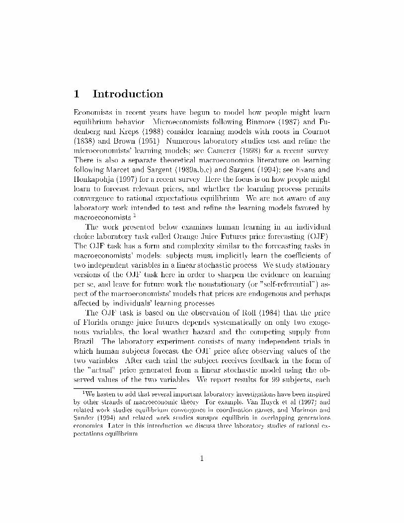
Apparatus. The experiment uses a graphics computer program writtenin C++, run on power Macintosh 7500/100 computers with full color moni-tors. Subjects in four sound dampened isolated testing rooms view controlledevents on the monitor screen and respond via clicking the mouse on variousicons on the display. See Figures 1.1-1.3 for examples of screen displays.This setup was chosen to minimize boredom and to eliminate the possibilityof peer pressure.
Stimuli. The realized values for weather x1t and supply x2t are indepen-dently drawn each period from the uniform distribution on [0; 100], so thevariables are orthogonal. The noise term is independently drawn each periodfrom a di�erent uniform distribution, U [�v; v]. The realized values then arecombined using equation (1) and chosen parameter values (a1; a2; and v) toproduce a 480 trial sequence of prices. The same sequence of realized valuesand prices is used for all subjects in any given treatment condition.
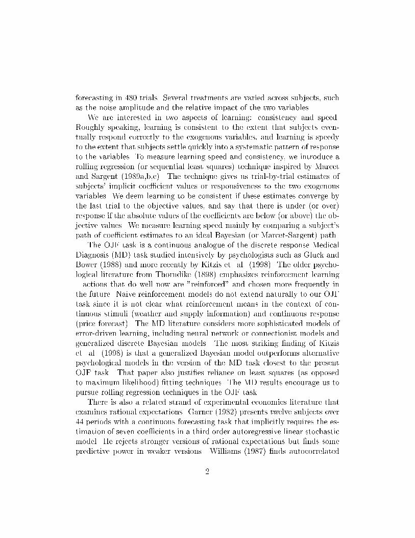
Method. Each trial begins with the graphical presentation of the weatherand supply values using two thermometer icons (labeled weather hazard andBrazilian supply) on the left side of the monitor display as in Figure 1.1(A). Each thermometer is partially �lled in red to indicate the realized value.Except in the no history treatment described below, the subject could alsoaccess (by clicking Previous Cases icon labelled (C) in Figure 1.1) the historyof prices in previous trials with similar weather and supply levels, as in Figure1.2 (D).2
2The history box (D) displays numerically the current realization of both variables, thenumber of previous trials for each variable whose realization is within 10 of the current
4

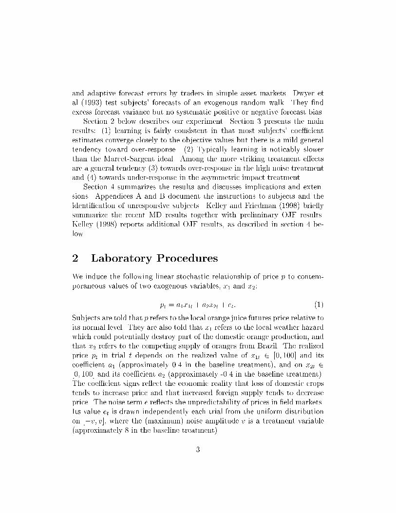
Subjects enter their forecast each period by moving slide (B) in Figure1.1 up or down within the possible price range. After the price predictionis entered and con�rmed, a blue line appears on the slide bar to indicatethe actual price in that trial as in Figure 1.3 (E). Except in the no scoretreatment described below, the score box then appears as in Figure 1.3 (F).3
After viewing the score box (if present) the subject advances to the next trialvia a mouse click.
Each subject completes 480 self-paced trials. The session is broken into3 blocks of 160 trials and subjects are permitted �ve minute breaks betweenblocks. Subjects generally �nish in less than the allotted two hours.
2.1 Treatments.
Baseline. The baseline parameter values are a1 = 0:417, a2 = �0:417 andv = 8:33. The history and score boxes appear as described above. Each trialthe score is calculated from the continuous price forecast c and the realizedprice p using the quadratic scoring rule S(p; c) = A�B(p� c)2, with A = 80and B = 280. Thus the maximum score (for a perfect forecast) is A = 80points and the minimum is �B = �200 points. See Friedman and Massaro(1998) for a recent discussion of this scoring rule. The box also displays the"expert" score of a forecaster with nothing left to learn, i.e., the score earnedby forecasting a1x1t + a2x2t in trial t, using objective values of ai. Subjects,of course, do not observe the expert forecast, just the expert score.
Paid. This treatment di�ers from baseline only in that subjects are paidaccording to their �nal scores. Each subject receives a $5.00 show up feecovering the �rst 30,000 points of �nal cumulative score. (Actual �nal scoresalways exceeded 30,000 with the top scores over 37,000.) Subjects also receivean additional dollar for each 700 points scored above 30,000. The medianpayment was about $15.00 with top payments about $16.50. Subjects aretold the payment procedures on arrival.
No Score. This treatment di�ers from baseline only in that subjects donot have access to the Results or Score box icon and box (F).
realization, and the average realized price in those previous trials. The box remains onthe screen until the subject clicks the OK icon.
3The score box (F) displays the subject's score on the current trial and the cumulativescore through the current trial. The calculation is explained in section 2.1 below.
5
No History. This treatment di�ers from baseline only in that subjects donot have access to the Previous Cases or History icon and box (C) and (D).
Asymmetric. Here the coe�cient values are a1 = 0:250 and a2 = �0:583.Thus the weather and the competing supply information no longer have equal(or symmetric) impact on OJF price.
High Noise. Here the noise amplitude is almost doubled, to v = 14:3, andthe coe�cient values ai are scaled to �0:357, as described below. All otherfeatures are as in the baseline treatment.
2.2 Data Processing.
The baseline values of ai are scaled as follows. Begin with unscaled valuesa�1 = 0:5 and a�2 = �0:5. Given noise amplitude v�, equation (1) implies thatthe unscaled price ranges from p� = 0:5(0) � 0:5(100) � v� = �[50 + v�] top� = 0:5(100)� 0:5(0) + v� = [50 + v�]. To �t in the screen's range [�50; 50]we display the scaled price p = 50p�
[50+v�]. The scaled coe�cients therefore are
ai =50a�
i
[50+v�]and the scaled noise amplitude is v = 50v�
[50+v�]. For the baseline
noise value v� = 10 we have v = 8:33 and ai = 0:833a�i = 0:417. The scaledcoe�cients used in the high noise (v� = 20) and asymmetric treatments arederived in a similar fashion.
For a given subsequence of trials (pt; x1t; x2t), t = t0; :::; T , we de�nethe ideal Bayesian (or Least Squares or Marcet-Sargent) learner by regress-ing pt on the independent variables x1t and x2t via ordinary least squares(OLS). The regression over this subsequence of trials yields coe�cient esti-mates a1T and a2T . The subsequences we consider consist of trials 1 to 160,2 to 161, ... ,320 to 480. Thus we obtain learning curves a1T and a2T forT = 160; 161; :::; 480, which can be interpreted as ideal subjective estimatesof the objective values a1 and a2. We refer below to these as the M-S learningcurves.
We use similar rolling regressions for human subjects. An actual subjectmay think of the task in various idiosyncratic ways | for example, he maybelieve that prices are serially correlated or that price is a nonlinear deter-ministic function of the exogenous variables, despite our instructions to thecontrary. Nevertheless, the analyst can summarize the subject's beliefs byseeing how he responds to the current stimuli xit, and can summarize thelearning process by seeing how the subject's response changes with experi-
6
ence. Our approach therefore is to reconstruct implicit beliefs using equation(1) and subjects' actual responses.
The reconstruction proceeds as follows. Take the subject's actual forecastct in trial t as the dependent variable, and run rolling regressions as beforeon the realized values xit, using a moving window of 160 consecutive trialswith the last trial T ranging from 160 to 480. Consistent and speedy learn-ing is indicated by rapid convergence of the coe�cient estimates aiT (as Tincreases) to the objective values ai. Obstacles to learning are suggested byslow convergence, convergence to some other value which represents over- orunder-response, or divergence of the coe�cient estimates.
Some details may be worth noting brie y. (1) In all the results reportedbelow, the intercept coe�cient a0 is constrained to its objective value ofzero. Excluding the intercept doesn't a�ect our main results but does it doesreduce clutter and improve statistical e�ciency. (2) In preliminary work weconsidered stretchable windows of data running from t = 1 to T , to capturefully the evidence available to the subject (or M-S ideal learner) in trial T .However, the entire learning curve then re ects the subject's initial responsepattern as well as the recent response pattern. We concluded that learningcurves would be more informative when estimated from a moving windowthat includes only the most recent responses. Of course, the recent responsesalready incorporate everything the subject has learned since the beginningof the session. (3) Lengthening a (non-stretchable) moving window reducesstandard errors in the coe�cient estimates, but also reduces the weight onthe most recent responses. After a cursory investigation of preliminary data,we settled on length 160 as a reasonable compromise.
3 Results
Figure 2 presents a sample of learning curves in each treatment. Each panelof the Figure shows the objective coe�cient values as a horizontal dottedline and shows the ideal M-S learning curves as thin continuous lines. Therolling regressions that generate the M-S curves seem to capture the pricedata quite well; typical R2s ranged from 0.91 for the �rst 160 trial window ofdata to 0.93 for the last window. We were pleased to see that M-S learningis consistent and quite rapid, indeed virtually complete within the �rst 160trials, as indicated by closeness of the dotted and thin continuous lines in
7
every panel. The gap between the lines typically is about one standard errorof the M-S coe�cient estimate.
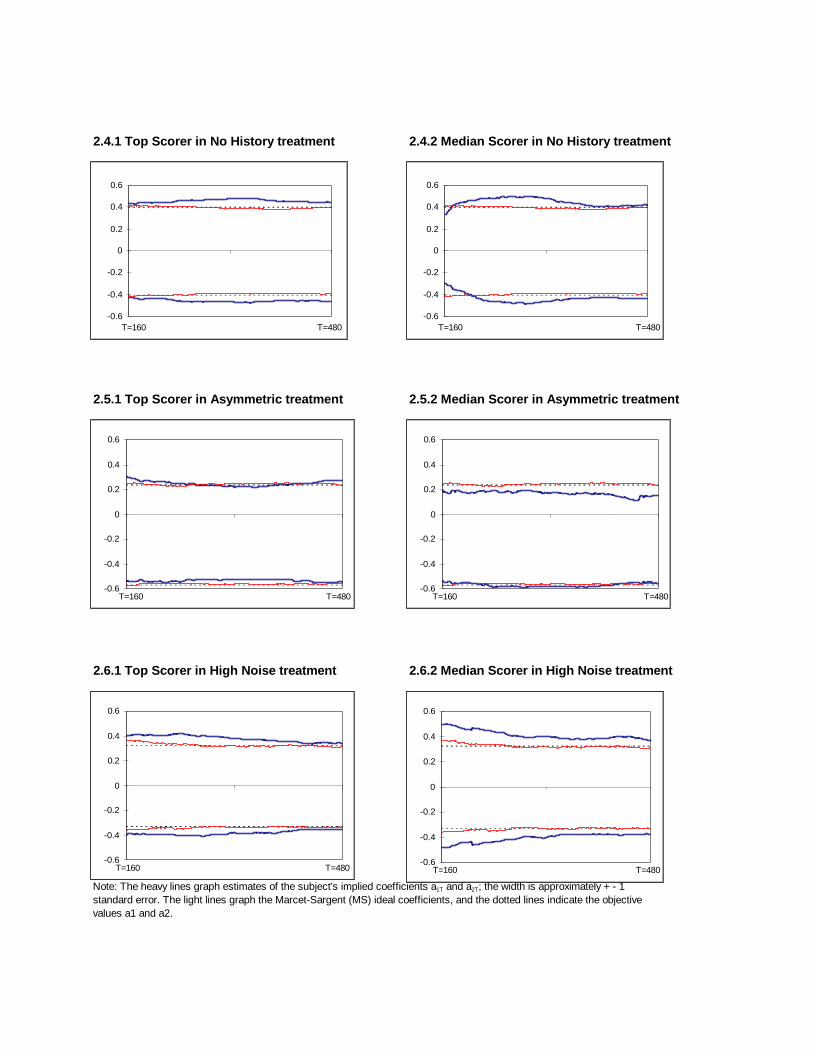
The heavy continuous lines in each panel of Figure 2 represent the learningcurves for the highest scoring subject or the subject with the median scorein each treatment. The corresponding rolling regressions again had typicalR2s above 0.90. The �rst two panels show moderate but persistent over-response to current weather and supply information, with implicit coe�cientestimates lying closer to�0.45 than to �0.42 for both subjects in the baselinetreatment. The next two panels suggest that the top scoring paid subjectis right on target, but the median scorer tends to under-respond slightly.Over-response seems strongest with the top scoring subject in the no historytreatment and the two subjects shown in the high noise treatment. Thetwo subjects shown in the asymmetric treatment appear to under-respond inmost trials.
To conserve space we do not show the learning curves for the other 87subjects. Su�ce it to say that subjects sometimes over-respond, sometimesunder-respond, but typically are fairly close to the objective values. Subjectsseem to update more slowly than the M-S ideal learner. The rest of thissection will test these impressions more systematically.
3.1 Distribution of Scores
Figure 3 shows the distribution of the scores earned by subjects in eachtreatment. Forecasts often are quite good; in most treatments the highestscore is close to 38,000, only a bit below the Marcet-Sargent ideal. The modalscore and the median score usually are not very far behind. Mean scores areusually lower because the lowest scores are much lower, sometimes below34,000. For comparison, we calculated scores in the baseline treatment fortwo sorts of zero intelligence agents or non-learners. An agent who alwaysforecasted zero (the optimal uninformed forecast) would score 34,326 and anagent who always used last period's price as the forecast would earn 30,647.
Closer examination of the raw data raises questions about the motivationof the subjects with lowest scores. We found that these subjects generallystopped responding to the weather and Brazil supply information at somepoint during the session. Subjects who don't care about performance butseek only to �nish quickly can do so by just clicking the "OK" icons in everytrial, leaving the price forecast at the default value c = 0. We identi�ed such
8
behavior in 9 of the 99 subjects. Note that unthinking responses of c = 0will bias the coe�cient estimates towards 0, so it is potentially important tothe data analysis to identify such "questionable" behavior. Appendix B liststhe questionable subjects and the criteria used to identify them.
Do the treatments systematically a�ect performance? Figure 3 suggeststhat, compared to the baseline treatment, scores may be a bit higher forpaid subjects and a bit lower in some of the other treatments. StandardWilcoxon tests indicate signi�cantly lower scores in the asymmetric (p-value= 0.002), and high noise (p=0.002) treatments, and no signi�cant di�erencefrom baseline in the no score (p=0.71), and no history (p=0.56) treatments.The paid condition produced insigni�cantly higher scores than the baseline(p=0.15).
3.2 Distribution of Coe�cient Estimates.
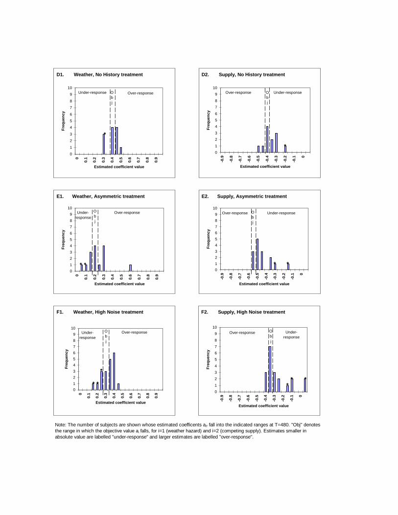
Figure 4 shows the �nal (T = 480) distribution of both coe�cient estimatesby treatment. Overall, the subjects seem to have it about right: the estimatescenter near the objective value and most of the estimates are not far away.Moreover, most of the outlying estimates are spurious under-responses fromthe 10 questionable subjects (denoted with asterisks (*)). The distributionsseem tighter in the paid treatment than in the baseline, and perhaps a bitmore dispersed in the last three treatments. More importantly, there may bea slight bias towards over-response in the high noise treatment and towardsunder-response in the asymmetric treatment.
Further analysis is required to explore these impressions. Table 1 classi�esa �nal (T=480) coe�cient estimate as objectively correct if its central 95%con�dence interval contains the corresponding �nal value from the Marcet-Sargent simulation.4 The estimate is classi�ed as over- (or under-) responseif the con�dence interval lies entirely outside (or entirely within) the intervalfrom zero to the (M-S) objective value. Overall, a plurality of estimates (71 ofthem) are classi�ed as objectively correct, and there are about equal numbersof over-responses (59) and under-responses (48 plus 18 questionables).
4Note that this rede�nition of the objective value uses the available sample informationrather than unavailable population information to de�ne the objective value. The original(population) de�nition di�ers by about .013, and would tend to shift the classi�cationsvery slightly towards over-response.
9
The main imbalances arise in the last two treatments. Under-responseto the more important variable (labelled [Brazil] Supply in Figure 4) andover-response to the other variable are quite prevalent in the asymmetrictreatment. In the high noise treatment, a majority of the non-questionableestimates for both coe�cients are classi�ed as over-response and none isclassi�ed as under-response.
The last column of the Table reports Wilcoxon p-values separately foreach of the two coe�cients in each treatment for the full sample (and inparentheses, for the reduced sample that excludes the 9 questionable sub-jects.) In three cases the tests reject (at the conventional p=0.05 level inthe reduced sample) the null hypothesis that the estimates center at theobjective value, in favor of the following one-sided alternatives. There is sig-ni�cant under-response to the Supply variable in the asymmetric treatment(p=0.00), and signi�cant over-response to both variables in the high noisetreatment (p=0.02,0.00). There is also marginally signi�cant over-responseto the Supply variable in the baseline treatment (p=0.08). The other casesof apparent under- and over-response do not produce signi�cant results inthis conservative test.
The impression of tighter distributions in the paid treatment is consistentwith signi�cant �ndings in other experiments (Smith and Walker, 1993) butturns out not to be signi�cant in our data according to standard parametricand non parametric tests. Of course, the sample size is not large, and itmay be worth noting that subjects with questionable motivation appeared inthe baseline (and high noise and asymmetric) treatment but not in the paidtreatment.
Table 1 also reports behavior observed halfway through the session, atT=240. Recall from Figure 2 the impression (con�rmed in omitted �gures forthe other subjects) that modest but shrinking over-response is quite typicalat this point. The Table shows that over-response at the halfway point indeedis somewhat more prevalent than at the end of the session, especially in thepaid and high noise treatments.
3.3 Summary
Several general conclusions emerge from the data analysis. Our human sub-jects do not learn as fast as an ideal Bayesian (or Marcet-Sargent econo-metrician), but even at the half-way point (T=240) of the experiment, the
10
coe�cient estimates indicate that responses are not very far from the mark.The overall tendency is towards over-response to the current information x1and x2, but this tendency almost disappears by the end (T=480) of the exper-iment. We conclude that learning in our experiment generally is reasonablyrapid and very consistent.
The treatments have modest but detectable impacts. Compared to thebaseline condition, fewer subjects in the paid treatment appear to have ques-tionable motivation and the scores and coe�cient estimates seem to havetighter distributions. Surprisingly, neither the no score treatment nor theno history treatment signi�cantly impaired the the subjects' scores or ac-curacy of the estimated coe�cients. The asymmetric treatment, however,signi�cantly lowered scores and pushed subjects signi�cantly towards under-response to the more important information and (insigni�cantly) towardsover-response to the less important information. The high noise treatmenthad the strongest impact: lower scores and over-response to both informationvariables.
4 Discussion and Future Work.
Existing literature can easily give the impression that humans typically makevery irrational choices in simple laboratory tasks; see Rabin (1998) for a re-cent thoughtful survey. In sharp contrast, our human subjects rather quicklylearn highly rational behavior in a nontrivial forecasting task. What accountsfor the divergent results?
In some ways our experiment makes it di�cult for subjects to be ratio-nal. The task is challenging in that the target variable, price, is stochasticand contingent on two independent variables. Another challenging aspectof our experiment is that we used psychology pool subjects, unpaid in mosttreatments. Irrational behavior exhibited by such subjects in some tasks dis-appears when subjects drawn from other pools are o�ered salient payments(Friedman and Sunder, 1994). With the exception of 9 of 99 subjects whosemotivation was questionable, our subjects behaved quite rationally.
But in other ways our experiment gives rationality its best shot. Thebasic task allows subjects to learn over a relatively long sequence of trials(480) in a stationary environment. Our laboratory setup encourages subjectsto draw on relevant intuitions about price determination and avoids features
11
that might suggest inappropriate heuristics. The visual interface encouragesrapid and unbiased processing of information and feedback. If anything, theinterface biases subjects towards under-response, since the default responseis 0 and the subject must move the slide up or down from that point. Thereduced sample used in some of the data analysis screened out the mostegregious cases of default response, but perhaps some slight bias remains5.Arguably our setup is more representative of economically important �eldenvironments than the some of the setups used in laboratory studies that�nd irrational behavior.
The rational behavior is fairly robust. Performance was not signi�cantlyimpaired in the no score and no history treatments, which eliminated usefulfeedback. Even in the asymmetric and high noise treatments, performancewas still quite good. Kelley (1998) reports several additional robustnesschecks. Speci�cations designed to capture prior beliefs and non-linear re-sponses detected some transient e�ects in many subjects, but for the mostpart these e�ects disappeared by the �nal trial. Tests allowing a non-zero in-tercept term (a0) for the asymmetric weights treatment were also performed.The main e�ect of this additional parameter was to eliminate the marginallysigni�cant overresponse observed for the smaller stimuli. The underresponseobserved for the larger stimuli remained signi�cant. Responses remainedfairly rational even in a treatment featuring a structural break.
An important extension of the work presented here, especially from themacroeconomics point of view, is to introduce self-referential price determi-nation. Marcet and Sargent (1989abc) study several linear stochastic mod-els where traders' expectations a�ect the actual price observed each period.They derive conditions on traders' learning processes (rolling regressions inessence) that ensure convergence of actual price to rational expectations equi-librium. It seems feasible to implement such economies in the laboratoryand (given some stronger assumptions than needed in the present paper)
5The most questionable remaining subject is 009 in the no history treatment. He madevery erratic choices until late in the session, spent no more time making choices than thescreened subjects (about half as long as most remaining subjects), and earned almost aslow a score as screened subjects. He was not screened out of the reduced sample becausehe entered mainly non-default responses, but his motivation is also questionable and hiscoe�cient estimates indicate dramatic under-response. Indeed, the relevant test wouldindicate marginally signi�cant over-response (to the second variable in the no historytreatment, p=0.08) if this subject were screened out of the sample.
12
to extract estimates of subjects' learning processes. We conjecture that theempirical models introduced in the present paper will continue to do well ina more complex self-referential setting.
We see two main lessons in the present results. The discussion so farhas emphasized the lesson that people can learn to make quite good fore-casts. The other lesson is that some slight but systematic biases remain.In particular, even after 480 trials, subjects still tended to over-respond tonews in the high noise environment. Slight individual biases might interactto produce economically important market biases (Akerlof and Yellen, 1985;Kelley, 1998). More theoretical and empirical work is needed to understandlearning in self-referential, nonstationary environments.
13
References
[1] Akerlof, G. and Yellen, J., 1985, Can Small Deviations from Rationalitymake Signi�cant Di�erences to Economic Equilibria?, American Eco-nomic Review 75:4.
[2] Binmore, K., 1987, Modeling Rational Players, Part I, Economics andPhilosophy 3, 179-214.
[3] Binmore, K., 1988, Modeling Rational Players, Part II, Economics andPhilosophy 4, 9-55.
[4] Brown, G., 1951, Iterated Solution of Games by Fictitious Play, ActivityAnalysis of Production and Allocation (Wiley: New York).
[5] Camerer, Colin, 1998, Experiments on Game Theory, Draft manuscript,(Caltech Division of Humanities and Social Sciences).
[6] Cournot, A., 1838, Researches sur les Principes Mathematiques de laTheorie Richesses, English edition, N. Bacon, ed., 1897, Researches intothe Mathematical Principles of the Theory of Wealth (MacMillan, NY).
[7] Dywer Jr., G., Williams, A., Battalio, R., and Mason, T., 1993, Tests ofRational Expectations in a Stark Setting, The Economic Journal 103,586-601.
[8] Evans, George W. and Honkapohja, Seppo, 1997, Learning Dynamics,University of Oregon Economics working paper. To appear in J. Taylorand M. Woodford, eds., Handbook of Macroeconomics (Elsevier, NY).
[9] Friedman, D. and Massaro, D., 1998, Understanding Variability in Bi-nary and Continuous Choice, Psychonomic Bulletin and Review, inpress.
[10] Friedman, D. and Sunder, S., 1994, Experimental Methods: a Primerfor Economists (Cambridge University Press).
[11] Fudenberg, D., and D. Kreps, 1988, A Theory of Learning, Experimen-tation, and Equilibrium in Games, mimeo (MIT).
14
[12] Garner, A., Experimental Evidence on the Rationality of Intuitive Fore-casters, 1982, Research in Experimental Economics 2, 113-128 (JAIPress).
[13] Gluck, M. A. and Bower, G. H., 1988, From Conditioning to CategoryLearning: An Adaptive Network Model, Journal of Experimental Psy-chology: General 117, 225-244.
[14] Hull, C., 1943, Principles of Behavior, (New York Appleton-Century-Crofts).
[15] Kelley, H., 1998, Bounded Rationality in the Individual Choice Exper-iment, Unpublished Thesis, Economics Department, University of Cali-fornia Santa Cruz.
[16] Kelley, H. and Friedman, D., 1998, Learning to Forecast Rationally,Prepared for Charles Plott and Vernon Smith, eds., Handbook of Ex-perimental Economics Results.
[17] Kitzis S., Kelley H., Berg E., Massaro D., Friedman D., 1998, Broaden-ing the Tests of Learning Models, forthcoming Journal of MathematicalPsychology.
[18] Marcet, A. and Sargent, T., 1989a, Convergence of Least Squares Learn-ing Mechanisms in Self Referential Linear Stochastic Models, Journal ofEconomic Theory 48, 337-68.
[19] Marcet, A. and Sargent, T., 1989b, Convergence of Least Squares Learn-ing in Environments with Hidden State Variables and Private Informa-tion, Journal of Political Economy 97, 1306-22.
[20] Marcet, A. and Sargent, T., 1989c, Least Squares and the Dynamics ofHyperin ation, In W. Barnett, J. Geweke, and K. Shell, eds., Chaos,Complexity, and Sunspots (Cambridge University Press).
[21] Marimon, Ramon and Sunder, Shyam, 1993, Indeterminacy of Equilibriain a Hyperin ationaryWorld: Experimental Evidence, Econometrica 61,1073-1107.
15

[22] Rabin, M., 1988, Psychology and Economics, Journal of Economic Lit-erature 34, 11-46.
[23] Roll, R., 1984, Orange Juice and Weather, American Economic Review74, 861-880.
[24] Sargent, T., 1994, Bounded Rationality in Macroeconomics (ClarendonPress Oxford).
[25] Smith, V. and Walker, J., 1993, Monetary Rewards and Decision Costin Experimental Economics, Economic Inquiry 31, 245-261.
[26] Thordike, E. L., 1898, Animal Intelligence: An experimental study ofthe associative processes in animals, Psychol. Monogr. 2.
[27] Van Huyck, J., Battalio R., and Rankin, F., 1997, On the Origin ofConvention: Evidence From Coordination Games, Economic Journal107 (442), 56-97.
[28] Williams, A. W., 1987, The Formation of Price Forecasts in Experimen-tal Markets, Journal of Money Credit and Banking 19, 1-18.
16
Appendix A: Instructions to Subjects
ORANGE JUICE FUTURES EXPERIMENTrevised 5/98
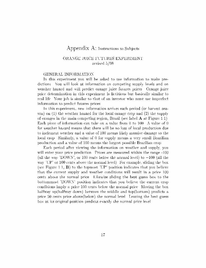
GENERAL INFORMATIONIn this experiment you will be asked to use information to make pre-
dictions. You will look at information on competing supply levels and onweather hazard and will predict orange juice futures prices. Orange juiceprice determination in this experiment is �ctitious but basically similar toreal life. Your job is similar to that of an investor who must use imperfectinformation to predict futures prices.
In this experiment, new information arrives each period (or harvest sea-son) on (1) the weather hazard for the local orange crop and (2) the supplyof oranges in the main competing region, Brazil (see label A at Figure 1.1).Each piece of information can take on a value from 0 to 100. A value of 0for weather hazard means that there will be no loss of local production dueto inclement weather and a value of 100 means likely massive damage to thelocal crop. Similarly, a value of 0 for supply means a very small Brazilianproduction and a value of 100 means the largest possible Brazilian crop.
Each period after viewing the information on weather and supply, youwill enter your price prediction. Prices are measured within the range -100(all the way 'DOWN', or 100 cents below the normal level) to +100 (all theway 'UP' or 100 cents above the normal level). For example, sliding the box(see Figure 1.1, B) to the topmost 'UP' position indicates that you believethat the current supply and weather conditions will result in a price 100cents above the normal price. Likewise sliding the best guess box to thebottommost 'DOWN' position indicates that you believe the current cropconditions imply a price 100 cents below the normal price. Moving the boxhalfway up(halfway down) between the middle and top(bottom) predicts aprice 50 cents price above(below) the normal level. Leaving the best guessbox at its original position predicts exactly the normal price level.
17
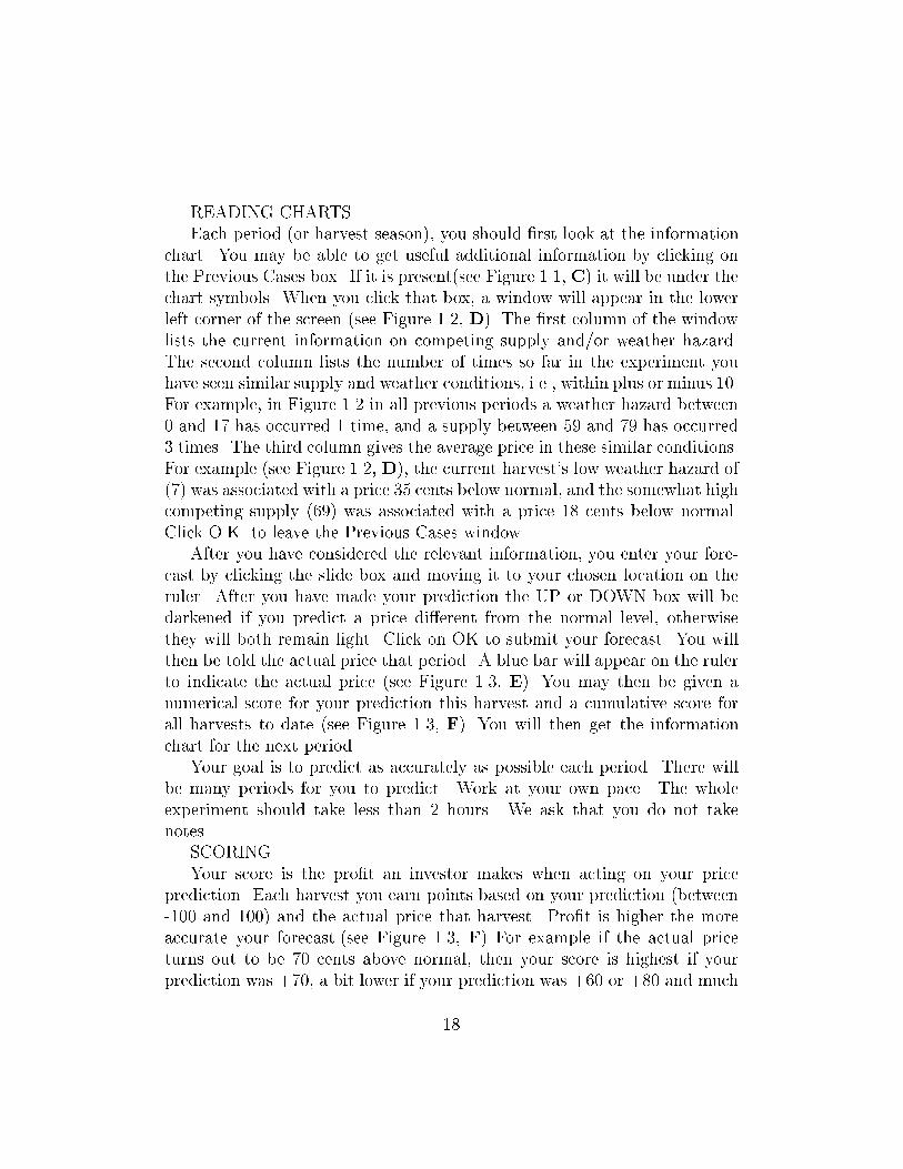
READING CHARTSEach period (or harvest season), you should �rst look at the information
chart. You may be able to get useful additional information by clicking onthe Previous Cases box. If it is present(see Figure 1.1, C) it will be under thechart symbols. When you click that box, a window will appear in the lowerleft corner of the screen (see Figure 1.2, D). The �rst column of the windowlists the current information on competing supply and/or weather hazard.The second column lists the number of times so far in the experiment youhave seen similar supply and weather conditions, i.e., within plus or minus 10.For example, in Figure 1.2 in all previous periods a weather hazard between0 and 17 has occurred 1 time, and a supply between 59 and 79 has occurred3 times. The third column gives the average price in these similar conditions.For example (see Figure 1.2, D), the current harvest's low weather hazard of(7) was associated with a price 35 cents below normal, and the somewhat highcompeting supply (69) was associated with a price 18 cents below normal.Click O.K. to leave the Previous Cases window.
After you have considered the relevant information, you enter your fore-cast by clicking the slide box and moving it to your chosen location on theruler. After you have made your prediction the UP or DOWN box will bedarkened if you predict a price di�erent from the normal level, otherwisethey will both remain light. Click on OK to submit your forecast. You willthen be told the actual price that period. A blue bar will appear on the rulerto indicate the actual price (see Figure 1.3, E). You may then be given anumerical score for your prediction this harvest and a cumulative score forall harvests to date (see Figure 1.3, F). You will then get the informationchart for the next period.
Your goal is to predict as accurately as possible each period. There willbe many periods for you to predict. Work at your own pace. The wholeexperiment should take less than 2 hours. We ask that you do not takenotes.
SCORINGYour score is the pro�t an investor makes when acting on your price
prediction. Each harvest you earn points based on your prediction (between-100 and 100) and the actual price that harvest. Pro�t is higher the moreaccurate your forecast.(see Figure 1.3, F) For example if the actual priceturns out to be 70 cents above normal, then your score is highest if yourprediction was +70, a bit lower if your prediction was +60 or +80 and much
18

lower if you predicted 0 or below.
19
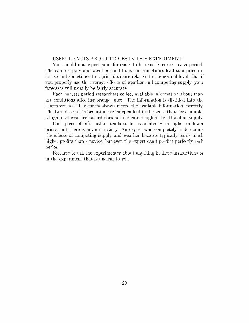
USEFUL FACTS ABOUT PRICES IN THIS EXPERIMENTYou should not expect your forecasts to be exactly correct each period.
The same supply and weather conditions can sometimes lead to a price in-crease and sometimes to a price decrease relative to the normal level. But ifyou properly use the average e�ects of weather and competing supply, yourforecasts will usually be fairly accurate.
Each harvest period researchers collect available information about mar-ket conditions a�ecting orange juice. The information is distilled into thecharts you see. The charts always record the available information correctly.The two pieces of information are independent in the sense that, for example,a high local weather hazard does not indicate a high or low Brazilian supply.
Each piece of information tends to be associated with higher or lowerprices, but there is never certainty. An expert who completely understandsthe e�ects of competing supply and weather hazards typically earns muchhigher pro�ts than a novice, but even the expert can't predict perfectly eachperiod.
Feel free to ask the experimenter about anything in these instructions orin the experiment that is unclear to you.
20
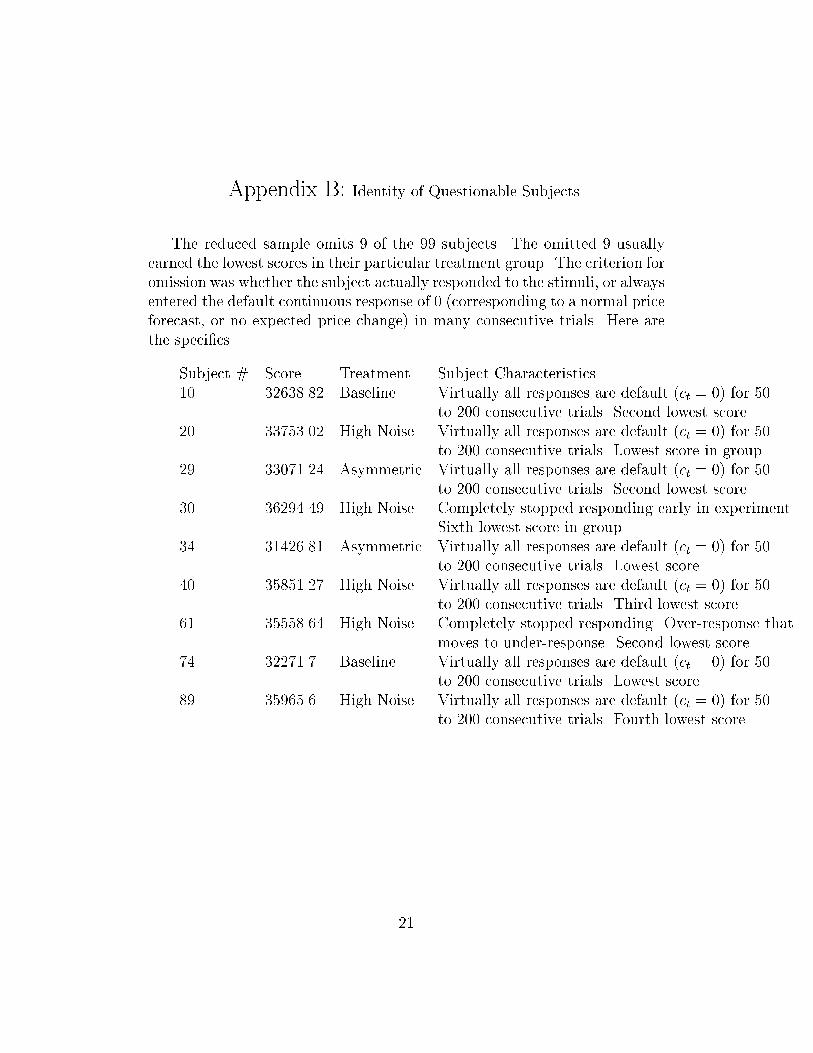
Appendix B: Identity of Questionable Subjects.
The reduced sample omits 9 of the 99 subjects. The omitted 9 usuallyearned the lowest scores in their particular treatment group. The criterion foromission was whether the subject actually responded to the stimuli, or alwaysentered the default continuous response of 0 (corresponding to a normal priceforecast, or no expected price change) in many consecutive trials. Here arethe speci�cs.
Subject # Score Treatment Subject Characteristics10 32638.82 Baseline Virtually all responses are default (ct = 0) for 50
to 200 consecutive trials. Second lowest score.20 33753.02 High Noise Virtually all responses are default (ct = 0) for 50
to 200 consecutive trials. Lowest score in group.29 33071.24 Asymmetric Virtually all responses are default (ct = 0) for 50
to 200 consecutive trials. Second lowest score.30 36294.49 High Noise Completely stopped responding early in experiment
Sixth lowest score in group.34 31426.81 Asymmetric Virtually all responses are default (ct = 0) for 50
to 200 consecutive trials. Lowest score.40 35851.27 High Noise Virtually all responses are default (ct = 0) for 50
to 200 consecutive trials. Third lowest score.61 35558.64 High Noise Completely stopped responding. Over-response that
moves to under-response. Second lowest score.74 32271.7 Baseline Virtually all responses are default (ct = 0) for 50
to 200 consecutive trials. Lowest score.89 35965.6 High Noise Virtually all responses are default (ct = 0) for 50
to 200 consecutive trials. Fourth lowest score.
21
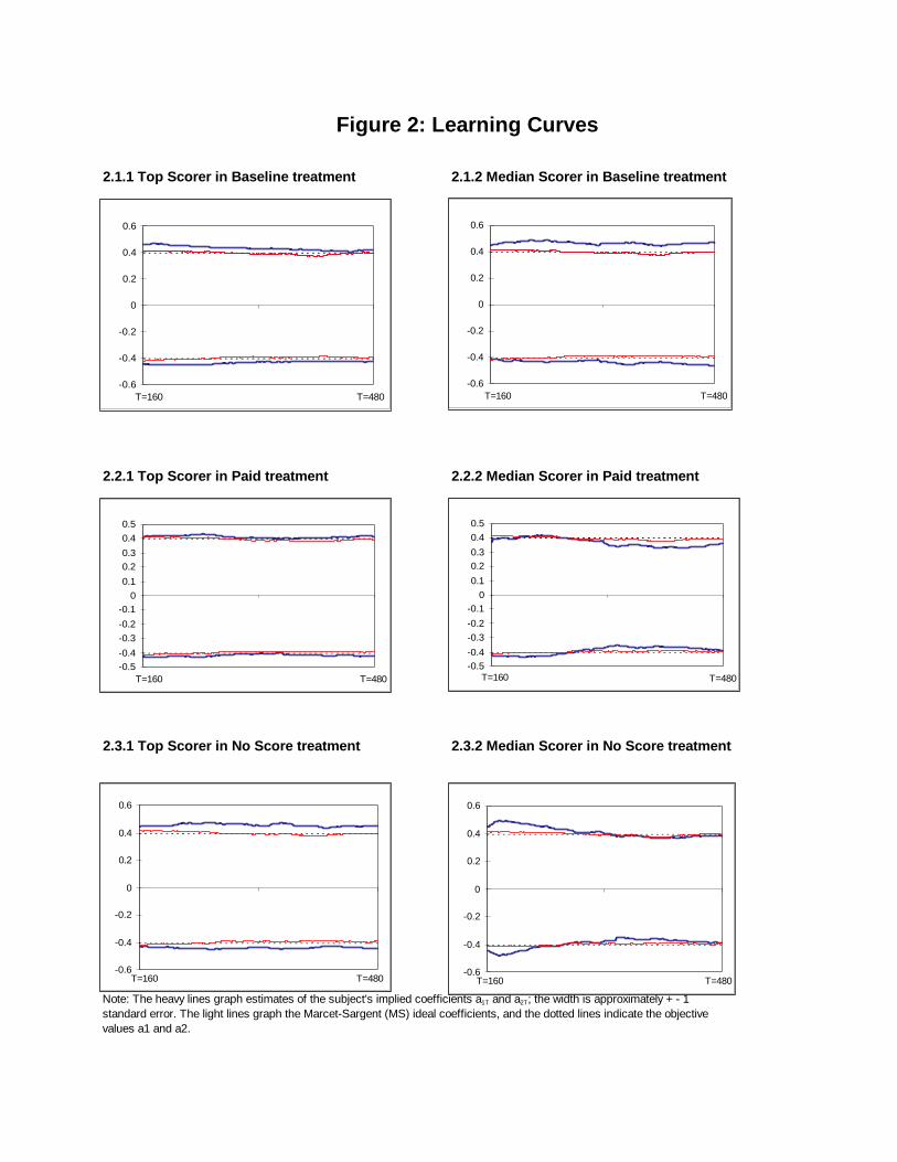
Figure 2: Learning Curves
2.1.1 Top Scorer in Baseline treatment 2.1.2 Median Scorer in Baseline treatment
2.2.1 Top Scorer in Paid treatment 2.2.2 Median Scorer in Paid treatment
2.3.1 Top Scorer in No Score treatment 2.3.2 Median Scorer in No Score treatment
Note: The heavy lines graph estimates of the subject's implied coefficients a1T and a2T; the width is approximately + - 1standard error. The light lines graph the Marcet-Sargent (MS) ideal coefficients, and the dotted lines indicate the objectivevalues a1 and a2.
-0.6
-0.4
-0.2
0
0.2
0.4
0.6
T=480T=160-0.6
-0.4
-0.2
0
0.2
0.4
0.6
T=480T=160
-0.5-0.4-0.3-0.2-0.1
00.10.20.30.40.5
T=160 T=480-0.5-0.4-0.3-0.2-0.1
00.10.20.30.40.5
T=480T=160
-0.6
-0.4
-0.2
0
0.2
0.4
0.6
T=160 T=480-0.6
-0.4
-0.2
0
0.2
0.4
0.6
T=480T=160
2.4.1 Top Scorer in No History treatment 2.4.2 Median Scorer in No History treatment
2.5.1 Top Scorer in Asymmetric treatment 2.5.2 Median Scorer in Asymmetric treatment
2.6.1 Top Scorer in High Noise treatment 2.6.2 Median Scorer in High Noise treatment
Note: The heavy lines graph estimates of the subject's implied coefficients a1T and a2T; the width is approximately + - 1standard error. The light lines graph the Marcet-Sargent (MS) ideal coefficients, and the dotted lines indicate the objectivevalues a1 and a2.
-0.6
-0.4
-0.2
0
0.2
0.4
0.6
T=480T=160-0.6
-0.4
-0.2
0
0.2
0.4
0.6
T=160 T=480
-0.6
-0.4
-0.2
0
0.2
0.4
0.6
T=480T=160-0.6
-0.4
-0.2
0
0.2
0.4
0.6
T=480T=160
-0.6
-0.4
-0.2
0
0.2
0.4
0.6
T=480T=160-0.6
-0.4
-0.2
0
0.2
0.4
0.6
T=480T=160
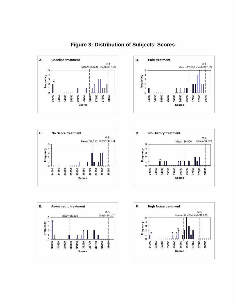
Figure 3: Distribution of Subjects' Scores
E. Asymmetric treatment
0
1
2
3
4
5
3400
0
3445
0
3490
0
3535
0
3580
0
3625
0
3670
0
3715
0
3760
0
3805
0
Scores
Freq
uenc
y
Mean=35,300|||||||
M-Sideal=38,107
| | | | | | |
*
F. High Noise treatment
0
1
2
3
4
5
3400
0
3445
0
3490
0
3535
0
3580
0
3625
0
3670
0
3715
0
3760
0
3805
0
Scores
Freq
uenc
y
Mean=36,400|||||||
M-Sideal=37,600
|||||||
* * **
C. No Score treatment
0
1
2
3
4
5
3400
0
3445
0
3490
0
3535
0
3580
0
3625
0
3670
0
3715
0
3760
0
3805
0
Scores
Freq
uenc
y
Mean=37,050 | | | | | | |
M-Sideal=38,103
| | | | | | |
A. Baseline treatment
0
1
2
3
4
5
3400
0
3445
0
3490
0
3535
0
3580
0
3625
0
3670
0
3715
0
3760
0
3805
0Scores
Freq
uenc
y
Mean=36,600||||||||
M-Sideal=38,103
| | | | | | | |
*
B. Paid treatment
0
1
2
3
4
5
3400
0
3445
0
3490
0
3535
0
3580
0
3625
0
3670
0
3715
0
3760
0
3805
0
Scores
Freq
uenc
y
Mean=37,000 | | | | | | |
M-Sideal=38,103
| | | | | | |
D. No History treatment
0
1
2
3
4
5
3400
0
3445
0
3490
0
3535
0
3580
0
3625
0
3670
0
3715
0
3760
0
3805
0
Scores
Freq
uenc
yMean=36,400
| | | | | | |
M-Sideal=38,103
| | | | | | |
*

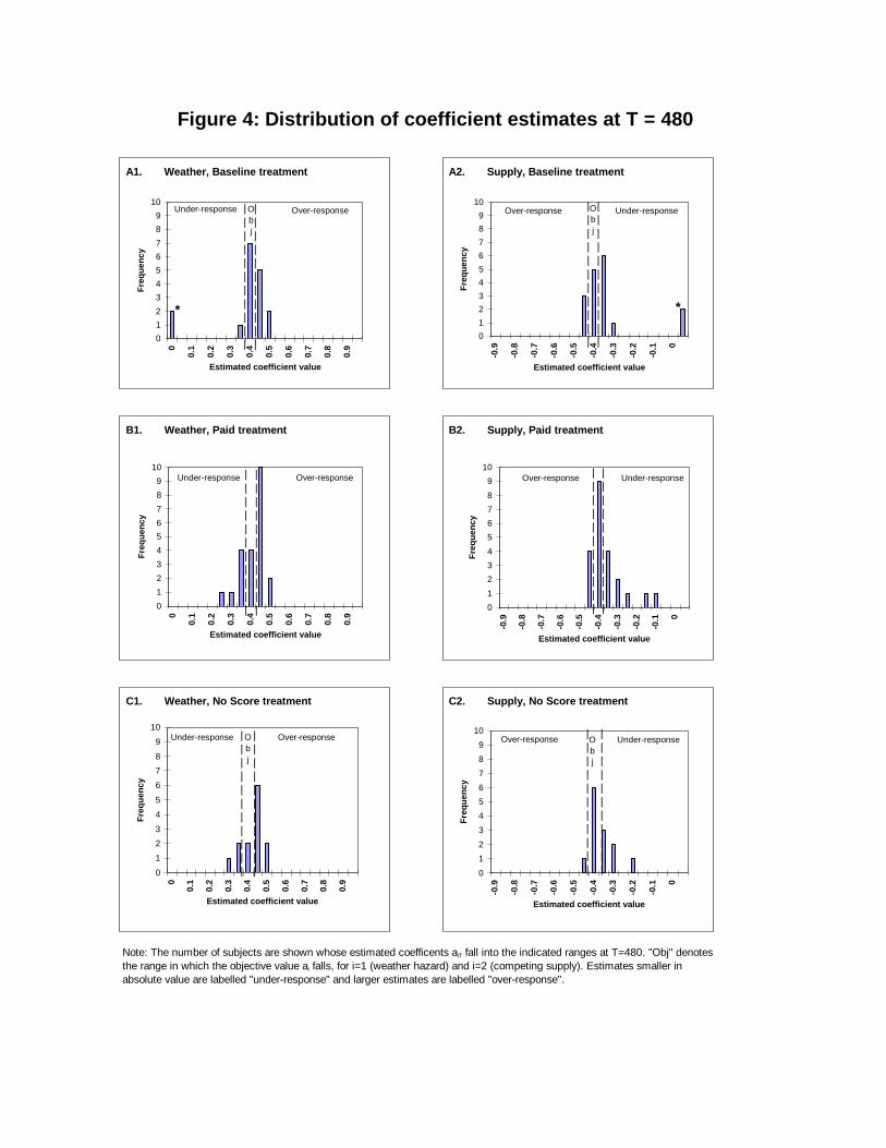
Figure 4: Distribution of coefficient estimates at T = 480
Note: The number of subjects are shown whose estimated coefficents aiT fall into the indicated ranges at T=480. "Obj" denotesthe range in which the objective value ai falls, for i=1 (weather hazard) and i=2 (competing supply). Estimates smaller inabsolute value are labelled "under-response" and larger estimates are labelled "over-response".
A1. Weather, Baseline treatment
012
34567
89
10
0
0.1
0.2
0.3
0.4
0.5
0.6
0.7
0.8
0.9
Estimated coefficient value
Freq
uenc
y
|||||||||||
|||||||||||
Obj
Under-response Over-response
*
A2. Supply, Baseline treatment
0123456789
10
-0.9
-0.8
-0.7
-0.6
-0.5
-0.4
-0.3
-0.2
-0.1 0
Estimated coefficient value
Freq
uenc
y
|||||||||||
|||||||||||
Obj
Under-responseOver-response
*
B1. Weather, Paid treatment
0
1
2
3
4
56
7
8
9
10
0
0.1
0.2
0.3
0.4
0.5
0.6
0.7
0.8
0.9
Estimated coefficient value
Freq
uenc
y
|||||||||||
|||||||||||
Over-responseUnder-response
B2. Supply, Paid treatment
0
1
2
3
4
5
6
7
8
9
10
-0.9
-0.8
-0.7
-0.6
-0.5
-0.4
-0.3
-0.2
-0.1 0
Estimated coefficient value
Freq
uenc
y|||||||||||
|||||||||||
Under-responseOver-response
C1. Weather, No Score treatment
0
1
2
3
4
5
6
7
8
9
10
0
0.1
0.2
0.3
0.4
0.5
0.6
0.7
0.8
0.9
Estimated coefficient value
Freq
uenc
y
Obj
Over-responseUnder-response |||||||||||
|||||||||||
C2. Supply, No Score treatment
0
1
2
3
4
5
6
7
8
9
10
-0.9
-0.8
-0.7
-0.6
-0.5
-0.4
-0.3
-0.2
-0.1 0
Estimated coefficient value
Freq
uenc
y
|||||||||||
|||||||||||
Obj
Under-responseOver-response
Note: The number of subjects are shown whose estimated coefficents aiT fall into the indicated ranges at T=480. "Obj" denotesthe range in which the objective value ai falls, for i=1 (weather hazard) and i=2 (competing supply). Estimates smaller inabsolute value are labelled "under-response" and larger estimates are labelled "over-response".
D1. Weather, No History treatment
0
1
2
3
4
5
6
7
8
9
10
0
0.1
0.2
0.3
0.4
0.5
0.6
0.7
0.8
0.9
Estimated coefficient value
Freq
uenc
y
|||||||||||
|||||||||||
Obj
Over-responseUnder-response
*
D2. Supply, No History treatment
0
1
2
3
4
5
6
7
8
9
10
-0.9
-0.8
-0.7
-0.6
-0.5
-0.4
-0.3
-0.2
-0.1 0
Estimated coefficient value
Freq
uenc
y
|||||||||||
|||||||||||
Obj
Over-response Under-response
*
E1. Weather, Asymmetric treatment
0
1
2
3
4
5
6
7
8
9
10
0
0.1
0.2
0.3
0.4
0.5
0.6
0.7
0.8
0.9
Estimated coefficient value
Freq
uenc
y
|||||||||||
|||||||||||
Obj
Over-responseUnder-response
* *
E2. Supply, Asymmetric treatment
01
23
45
67
89
10
-0.9
-0.8
-0.7
-0.6
-0.5
-0.4
-0.3
-0.2
-0.1 0
Estimated coefficient value
Freq
uenc
y|||||||||||
|||||||||||
Obj
Over-response Under-response
* *
F1. Weather, High Noise treatment
01
23
456
78
910
0
0.1
0.2
0.3
0.4
0.5
0.6
0.7
0.8
0.9
Estimated coefficient value
Freq
uenc
y
|||||||||||
|||||||||||
Obj
Over-responseUnder-response
* *
*
F2. Supply, High Noise treatment
0
1
2
3
4
5
6
7
8
9
10
-0.9
-0.8
-0.7
-0.6
-0.5
-0.4
-0.3
-0.2
-0.1 0
Estimated coefficient value
Freq
uenc
y
|||||||||||
|||||||||||
Obj
Over-response Under-response
***