Embed Size (px)
Citation preview
Learning to Believe in SunspotsAuthor(s): Michael WoodfordSource: Econometrica, Vol. 58, No. 2 (Mar., 1990), pp. 277-307Published by: The Econometric SocietyStable URL: http://www.jstor.org/stable/2938205 .
Accessed: 25/11/2013 12:53
Your use of the JSTOR archive indicates your acceptance of the Terms & Conditions of Use, available at .http://www.jstor.org/page/info/about/policies/terms.jsp
.JSTOR is a not-for-profit service that helps scholars, researchers, and students discover, use, and build upon a wide range ofcontent in a trusted digital archive. We use information technology and tools to increase productivity and facilitate new formsof scholarship. For more information about JSTOR, please contact [email protected].
.
The Econometric Society is collaborating with JSTOR to digitize, preserve and extend access to Econometrica.
http://www.jstor.org
This content downloaded from 128.59.154.119 on Mon, 25 Nov 2013 12:53:40 PMAll use subject to JSTOR Terms and Conditions

Econometrica, Vol. 58, No. 2 (March, 1990), 277-307
LEARNING TO BELIEVE IN SUNSPOTS
BY MICHAEL WOODFORD1
An adaptive learning rule is exhibited for the Azariadis (1981) overlapping generations model of a monetary economy with multiple equilibria, under which the economy may converge to a stationary sunspot equilibrium, even if agents do not initially believe that outcomes are significantly different in different "sunspot" states. The type of learning rule studied is of the "stochastic approximation" form studied by Robbins and Monro (1951); methods for analyzing the convergence of this form of algorithm are presented that may be of use in many other contexts as well. Conditions are given under which convergence to a sunspot equilibrium occurs with probability one.
KExwoRDs: Sunspots, learning, stochastic approximation, overlapping generations.
A NUMBER OF AUTHORS have shown that competitive economies may possess "sunspot equilibria", that is, rational expectations equilibria in which purely extrinsic uncertainty affects equilibrium prices and allocations.2 Such results demonstrate that it does not require a lack of faith in the rationality of market participants to believe that competitive markets may be subject to purely specula- tive fluctuations, driven solely by expectations.3
The mere existence of sunspot equilibria as solutions to a system of market- clearing conditions, however, might not be judged sufficient to indicate that competitive markets with rational participants could ever be subject to specula- tive instability. The sunspot equilibria represent states of affairs in which agents act differently in the case of different realizations of the "sunspot" variable, and it is rational for each agent to do so. But it might be thought unlikely that the beliefs of all the participants in the market could ever come to be coordinated so as to bring about an equilibrium of that kind. It is rational to believe that sunspots convey information about future states of affairs once the economy is in a sunspot equilibrium, but why would rational agents ever begin to believe in such a thing, so as to create the conditions under which the belief is rational?
In order to address such a question, one must go beyond the mere statement of the conditions for equilibrium and discussion of what states of affairs satisfy them; one must specify an explicit dynamic process according to which the beliefs of agents adjust when out of equilibrium. Any exercise of this kind is necessarily unsatisfactory, as there is no univocal meaning for the postulate of "rational" behavior outside of an equilibrium. It may well be the case that
1 I would like to thank Michele Boldrin, Jean-Michel Grandmont, Roger Guesnerie, and Jose Scheinkman for helpful discussions, and several referees for useful comments on earlier drafts. I would also like to thank the National Science Foundation for research support, and the Institute of Economic Analysis, Universitat Autonoma de Barcelona, for its hospitality during the preparation of this draft.
2 The earliest examples of sunspot equilibria in general equilibrium models were given by Shell (1977) and Cass and Shell (1983). Equilibria of this kind in ad hoc macroeconomic models were previously exhibited by Black (1974), Taylor (1977), and Shiller (1978), among others. Other general equilibrium examples are cited in Section 1.
3 For discussion of the potential relevance of such models for equilibrium business cycle theory, see Woodford (1987a, 1988).
277
This content downloaded from 128.59.154.119 on Mon, 25 Nov 2013 12:53:40 PMAll use subject to JSTOR Terms and Conditions

278 MICHAEL WOODFORD
different "learning" processes-all equally plausible or implausible, in that all satisfy some weak criteria for rational decision-making and all involve quite arbitrary choices-yield different conclusions as to the stability of a given equilibrium. Yet there seems no other way to address doubts about the economic significance of sunspot equilibria. And the exercise is not without value, even when it must be inconclusive. An example of instability of the nonsunspot rational expectations equilibrium, even for a particular learning rule, indicates that a coherent story can be told in which speculative instability arises in a competitive economy. And contrariwise, an example of stability of the non- sunspot equilibrium even when sunspot equilibria exist would indicate that competitive economies may be less subject to speculative fluctuations than a mere consideration of the set of equilibria would suggest.
Lucas (1986) has proposed that stability under disequilibrium learning dynam- ics of the kind modeled here be used as a criterion to decide which of the many rational expectations equilibria in an overlapping generations model of fiat money should be considered more likely to actually occur. He conjectures that the unique equilibrium in which the quantity theory of money is valid (i.e., in which the price level is constant, given a constant money supply) is the one to which agents should converge, and gives an example of a simple learning process with this property. Here we consider this problem again, in the case of a more complicated learning process, in which agents are willing ex ante to consider the possibility that a "sunspot" variable might be useful in forecasting the rate of return upon holding money. We find conditions under which the Lucas conjec- ture continues to be upheld, but also others under which the quantity-theoretic equilibrium (what we call the "monetary steady state") is unstable and the economy converges to a sunspot equilibrium instead.
In Section I, we review the Azariadis (1981) example of a simple infinite horizon general equilibrium model for which stationary sunspot equilibria may exist. In Section II, we introduce a plausible rule by which agents in this economy might seek to learn whether the sunspot variable is of any use in forecasting future variables of interest to them, and in Section III we present our results on the convergence of the dynamics generated by this learning process to rational expectations equilibrium. We exhibit conditions under which the nonsunspot stationary equilibrium is unstable under the learning process, and under which the process must converge to one of a certain set of sunspot equilibria. Section IV offers concluding remarks.
1. STATIONARY SUNSPOT EQUILIBRIA IN THE AZARIADIS MODEL
The example of an infinite horizon economy with stationary sunspot equilibria considered here was first presented by Azariadis (1981). The analysis of this example has subsequently been extended by Azariadis and Guesnerie (1982, 1986), Spear (1983), Chiappori and Guesnerie (1989), and Grandmont (1986, 1989). We choose to consider this example not only because it is so well known,
This content downloaded from 128.59.154.119 on Mon, 25 Nov 2013 12:53:40 PMAll use subject to JSTOR Terms and Conditions

SUNSPOTS 279
but because models with stationary sunspot equilibria of this kind are of interest for modeling repetitive "business cycle" fluctuations.4
Consider a stationary overlapping generations exchange economy in which all agents live for two consecutive periods, there is a single perishable consumption good for each period, and fiat money is the only asset. Let us suppose further that all agents have identical preferences, represented by a utility function u(c) -v(n), where n is the amount of labor supplied during the first period of life, and c is the amount of the single good consumed during the second period of life.5 The good is produced at constant returns to scale using the labor of the young, and units are chosen so that one unit of labor produces one unit of the good.
The utility function is assumed to satisfy the following assumptions:
ASSUMPTION (A.1): u, v are C2; u(c) is defined for all c> 0, v(n) for all 0 < n <n< .
ASSUMPTION (A.2): u' > 0, u" < 0, v' > 0, v" > 0, for all c, n in the above domains.
ASSUMPTION (A.3): v'(n) oo as n n.
ASSUMPTION (A.4): U'(c) oo as c 0.
The differentiability assumed in (A.1) is necessary in order for us to be able to use results from the stability analysis of smooth dynamical systems in analyzing convergence in Section 3. Conditions (A.2) state that preferences are monotone and concave in consumption and leisure. The upper bound on labor supply assumed in (A.3) is inessential, since we assume below that agents have beliefs that would result in a bounded labor supply in any event. Condition (A.4) is the
4It will be apparent that the method of analysis of learning dynamics employed here will in fact apply to a broader class of models of which this one is an example. The only properties of the model needed are that agents choose a state variable n, based upon forecasts of a variable R,+1 so as to maximize the expected value of a criterion function V(n,, R,+) that is concave in n,, and that the equilibrium value of R, +l be determined by agents' choices according to a smooth function R, = R(n,, n,+l).
5 This specification follows Azariadis (1981). A model in which agents supply labor and consume in both periods of life results in equilibrium conditions of the same form as those derived here, so that extension of the model to that case is trivial. See, e.g., Grandmont (1986). In that case, n, in the equations below is to be interpreted as excess supply by the young (i.e., labor supplied in excess of their own consumption), and c, as excess demand by the old.
The model presented here also has a structure quite similar to the cash-in-advance monetary economy of Lucas and Stokey (1987), in the case of no endowment shocks or money growth shocks. (On the existence of stationary sunspot equilibria in the Lucas-Stokey model, see Woodford (1987b, sec. 2A).) Hence the results of this paper immediately indicate that adaptive learning dynamics may converge to stationary sunspot equilibria in that model as well. Such an interpretation of our analysis here would be especially attractive since in that case the same agent would be adjusting his estimates from period to period in response to new data, rather than successive generations modifying the beliefs of their predecessors and since in that case it would be more plausible to assume that the structure of the economy could remain fixed for a large number of "periods."
This content downloaded from 128.59.154.119 on Mon, 25 Nov 2013 12:53:40 PMAll use subject to JSTOR Terms and Conditions

280 MICHAEL WOODFORD
only assumption that is at all restrictive; this condition guarantees that desired labor supply (and hence desired real balances) will be positive regardless of the rate of return expected on money.
A young agent in period t expecting a (possibly stochastic) real return R,?1 on fiat money held from period t to period t + 1, chooses his labor supply n, to maximize
(1.1) Et[u(n,R,+?) - v(n,)]
where Et denotes the expectation of agents in period t. (Throughout, we assume that all agents form expectations in the same way.) Since (1.1) is a concave function of n,, the optimal labor supply is the unique n, satisfying
(1.2) v'(n,) = Et [R?+lu'(n,R,+?)] -
We assume a constant supply of fiat money M > 0. This must be held by the old at the beginning of each period; hence the consumption demand each period is c, = M/pt, where p, is the price of the period t good in terms of money. Goods market clearing then implies n, = M/p, as well, so that R?+1 =ptlpt+ = n + In- In a rational expectations equilibrium, agents' expectations about the distribution of Rt+1 must coincide with the true conditional distribution for n+ 1/n, so that (1.2) implies
(1.3) n,v'(n,) = Et [n,+ju'(n+?)] .
A stationary rational expectations equilibrium (s.r.e.e.) is then a stationary stochastic process for n, that satisfies (1.3).
One stationary equilibrium is n, = n* for all t, where n* is the unique solution to u'(n*) = v'(n*). ((A.1)-(A.4) imply that the solution exists, is unique, and satisfies 0 < n* < n.) This is the familiar monetary steady state of the overlapping generations model of fiat money, the equilibrium that is consistent with the quantity theory of money. If lim c cu'(c) = 0, then another stationary solution is nt = 0 for all t. This is the familiar nonmonetary (autarchic) steady state of the overlapping generations model. These are the only equilibria in which n, is constant. Azariadis shows that there may also exist s.r.e.e. in which prices and allocations are stochastic, despite the absence of any random element in prefer- ences, endowments, or technology.
Azariadis considers the case in which agents observe a random variable s, (the "sunspot" variable), which takes a finite number of values {1,..., m } and follows a Markov process with transition probabilities 7Tij > 0 for i, j = 1, ..., m (Oij =
probability of moving to state j from state i). The sunspot variable has no effect upon the economy except through agents' expectations that may be conditioned upon it. He considers the existence of stationary rational expectations equilibria in which n = ni whenever s,= i, for i = 1,..., m. In this case, (1.3) becomes a system of m coupled equations for (nl,..., nm):
(1.4) n1v'(nj) = F,gjknku (nk) k
This content downloaded from 128.59.154.119 on Mon, 25 Nov 2013 12:53:40 PMAll use subject to JSTOR Terms and Conditions

SUNSPOTS 281
for j= 1,..., m. A stationary sunspot equilibrium is any s.r.e.e. (i.e., solution to (1.4)) in which ni # ni for some i, j.
If we define, for any vector n E (0, nf)f, the vector F by
(1.5) Fj(n) = nJ >'T'jknku'(nk) -v'(n), k
then s.r.e.e. in which money is always valued are just zeroes of F. Our assump- tions (A.1)-(A.4) on preferences imply the following.
LEMMA 1: There exists an n > 0 such that 0 < nk < n, and nk < ni < n for all j#k, imply Fk(n)>O.
PROOF: It follows from (A.2) and (A.4) that for any k,(1 -nkk)u(f) +
7Tkku'(n) - v'(n) is positive for small enough n. Choose n > 0 such that this is so. Then under the hypothesis, Fk(n) is at least as large as this expression, since n u'(n) > nku'(f) for all j 0 k.
LEMMA 2: There exists an n <n such that n < nk < n, and n < ni < nk for all j#k, imply Fk(n)<O.
PROOF: It follows from (A.2) and (A.3) that for any k, (1 - 7Tkk)u'(n) +
7Tkku'(n) - v'(n) is negative for n close enough to n. Choose n- < n such that this is so. Then under the hypotheses, Fk(n) is no greater than this expression, since nju'(nj) < nku'(n) for all j # k.
These results imply that F has no zeroes, apart from the origin, other than in (n, n-)m. Accordingly, stationary sunspot equilibria, if they exist, lie within that set.
Azariadis and Guesnerie (1982) establish the following sufficient condition for the existence of stationary sunspot equilibria, in the case m = 2, and the result is easily seen to extend to general m.
PROPOSITION 1: Let A(n) (- 1)I Det DF(n). If A(n*) <0, there exist sta- tionary sunspot equilibria. (Here we use n* to represent the m-vector whose elements all equal n*, i.e., the monetary steady state.)
Given Lemmas 1 and 2, this result follows immediately from the Poincare-Hopf index theorem,6 as in the argument of Azariadis and Guesnerie.
They also establish the following sufficient condition in terms of preferences alone:
PROPOSITION 2: If
(1.6) n*v"(n*) + n*u"(n*) + 2u'(n*) < ,
6 See Milnor (1965). For applications of this theorem to general equilibrium theory, see Mas-Colell (1985, pp. 188-222).
This content downloaded from 128.59.154.119 on Mon, 25 Nov 2013 12:53:40 PMAll use subject to JSTOR Terms and Conditions

282 MICHAEL WOODFORD
then there exist sets of transition probabilities rij > 0 such that A(n*) < 0. Thus there exist sunspot variables for which stationary sunspot equilibria exist.
PROOF: If (1.6) holds, A(n*) < 0 for the probabilities r12 = 1, 0lj= ? for all j = 2, rjl = 1 for all j # 1, and 'Tjk = 0 for all j, k # 1. By continuity, A continues to be negative even when the zeroes are made small positive quantities.
Condition (1.6) is just the condition for perfect foresight equilibrium to be indeterminate near the monetary steady state, i.e., for there to exist a continuum of perfect foresight equilibria all converging asymptotically to the monetary steady state.7 As it is well known that such a continuum of equilibria may exist, even in the case that both leisure and second-period consumption are normal goods (see Woodford (1984)), condition (1.6) is satisfied by a nonempty open set of economies.
For technical reasons, connected with the analysis of learning dynamics below, it is convenient to modify the Azariadis model by introducing preference shocks. Let us suppose that the disutility of labor for the young in period t is in fact given by v(nt) - Etnt, where v is a function with the properties assumed above, and Et is an independently and identically distributed (i.i.d.) random variable with bounded support, mean zero, and variance a 2 > 0. Let us also assume that the variables { e t} are independent of the sunspot process { st }. Finally, let us suppose that Et is only observed after labor supply nt has been chosen. Then (1.2) becomes
(1.7) v'(n,) = Et[Rt+lu'(ntR,+l) + Et].
In the case of a rational expectations equilibrium, Et(et) = 0, the true conditional expectation, and (1.7) is identical to (1.2). Hence the set of s.r.e.e. is still the zeroes of the vector function F defined in (1.5); and Propositions 1 and 2 still give sufficient conditions for the existence of stationary sunspot equilibria.
The taste shocks become significant, however, when we examine learning. We assume that agents also must learn the relevant properties of the distribution of taste shocks. Particular realizations of { Et } cause fluctuations in agents' estimates of the mean of the distribution. This is a source of variation in agents' behavior, early in the learning process, even if they do not believe that the sunspot states matter and do not behave differently in different sunspot states. This small (but unavoidable) variation in agents' behavior creates small fluctuations in the rate of return to holding money that will in general exhibit some small, accidental, sample correlation with the sunspot process. This sample correlation allows a belief in some small degree of significance of sunspot process for forecasting rates of return to arise, although it is clear that, unless such a belief is self-confirming (i.e., causes behavior that results in data that confirm and even strengthen the belief), the agents will asymptotically cease to hold such a belief, since the sample
7It can be shown, in fact, using the method of Woodford (1986b), that when (1.6) holds, stationary sunspot equilibria exist in the case of any stationary sunspot variable st, if nt is allowed to depend upon the entire history (s,, S- 1. . . ) rather than only upon the current St.
This content downloaded from 128.59.154.119 on Mon, 25 Nov 2013 12:53:40 PMAll use subject to JSTOR Terms and Conditions

SUNSPOTS 283
correlation will eventually become negligible unless it has ceased to be accidental. If we did not assume the small shocks to fundamentals, on the other hand, it might be possible for the economy to remain forever at a s.r.e.e. that is unstable (in the sense that small deviations from equilibrium beliefs would be self-con- firming if they ever occurred), simply because nothing ever occurs to perturb the equilibrium beliefs. Since in real economies fundamentals are always subject to at least small random variations, the case we consider is surely the one of greatest interest.
2. AN ADAPTIVE LEARNING PROCESS
We now wish to consider a process by which agents might come to have the beliefs characteristic of one or another of the s.r.e.e. described above. Equation (1.7) will continue to characterize optimal labor supply nt, but now the operator Et will be taken to refer to the subjective beliefs of agents in period t about the distributions from which Rt+1 and -, will be drawn; it may not correspond to the true conditional expectation as predicted by our model. Given a particular specification of how agents' expectations regarding that distribution evolve in response to observations of the rate of return on money, we have a complete model of how the economy will evolve. Expectations regarding R,+1 and Et
determine nt via (1.7), Rt= nt/nt-, provides another observation of the rate of return on money, et provides another observation of the taste shock, expectations in period t + 1 regarding Rt+2 and Et+, are adjusted accordingly, these then determine nt+l, and so on. We wish to consider whether such a process may result in convergence to one or another of the s.r.e.e.
The result, of course, depends upon how agents' expectations are assumed to evolve. We suppose that agents believe that the process generating rates of return upon money holdings belongs to a certain class M of statistical models, and that they use standard statistical procedures to determine which model in that class best fits the observed data (or, at any rate, to determine those parameters relevant to their decision problem). We also suppose that in each period they take the action that represents their current estimate of the optimal action. Some might regard these behavioral assumptions as less than fully "rational." After all, the maintained hypothesis that the true model belongs to class M is not correct, at least until convergence to a s.r.e.e. occurs, in the model presented here; the true model is a complicated nonstationary process, since the distribution of values for Rt+1 changes as the agents' beliefs evolve.
But in this respect the learning process examined here is like those considered for other types of dynamic economic models by Cyert and DeGroot (1974), Bray (1982, 1983), Bray and Savin (1984), and Marcet and Sargent (1986, 1987). Indeed, no model that seriously attempts to model behavior under an assumption of total ignorance about the equilibrium behavior of prices can avoid being unsatisfactory in this respect. Attempts to model "rational learning," such as those of Townsend (1983a, 1983b) or Bray and Kreps (1987), require an assump- tion of pre-existing coordination of agents' beliefs at some level, e.g., in
This content downloaded from 128.59.154.119 on Mon, 25 Nov 2013 12:53:40 PMAll use subject to JSTOR Terms and Conditions

284 MICHAEL WOODFORD
Townsend's case, common knowledge of a certain covariance matrix describing the joint distribution of agents' beliefs.8
The interest of an exercise of the kind presented here does depend, of course, upon an appropriate choice of the class of statistical models M. Certainly M must include the pattern of rates of return characteristic of some s.r.e.e.; otherwise, one would trivially obtain the result that convergence to a s.r.e.e. never occurs, but one would certainly want to question why agents should not eventu- ally discard the maintained hypothesis of class M. Secondly, M must be rich enough so that if agents maintain a belief in any model belonging to M other than one corresponding to a s.r.e.e., their actions will eventually produce observa- tions such that some other model belonging to M gives a better fit. That is, we do not wish for it to be possible for a model I to be the element of M best fitting the data generated by belief in u unless IL is the true model induced by belief in It.
Finally, in order to address the issue of interest to us here, the class M must include both the monetary steady state and at least some stationary sunspot equilibria, so that convergence to neither is ruled out a priori. An exercise of this kind is, in our view, more interesting in a case where there are multiple rational expectations equilibria to which the learning process might converge, than in the case more often considered, where there is only one. For in the usual case, if the analysis indicates that the learning process fails to converge to the rational expectations equilibrium, one may well conclude that agents will not in fact follow the postulated rule of inference forever, as they should eventually realize that their forecasts are not becoming more accurate despite the accumulation of data.9 In the case of multiple equilibria, by contrast, it is possible for one equilibrium to be found to be unstable under a learning process that nonetheless converges to another equilibrium, so that agents need not ever modify their rule of inference.
The interest of the exercise also depends, obviously, upon the rule by which agents are assumed to determine which element of M best fits the observed data. Any sort of outcome might be produced by assuming a sufficiently foolish rule of "inference." Certainly one must assume that agents use a consistent estimator, i.e., one such that, if their maintained hypothesis were true, would eventually result in their beliefs converging to the true model. (This, of course, does not assume away the problem of convergence to rational expectations, since during the learning process the maintained hypothesis will not be true.) It will also be noted below that the method of estimation assumed here represents a standard
8See Bray and Kreps (1987) for further discussion. They point out that an assumption of fully "rational learning" is possible only in the case of an analysis of how agents learn the value of certain parameters within a rational expectations equilibrium that is assumed to exist, not in the case of an attempt to model how the degree of coordination of expectations represented by such an equilibrium is attained. For an early discussion of why "rational learning" is not implied by the simple assumption that agents are fully rational, see Frydman (1982).
9See, e.g., the comment of Marcet and Sargent (1986, footnote 11).
This content downloaded from 128.59.154.119 on Mon, 25 Nov 2013 12:53:40 PMAll use subject to JSTOR Terms and Conditions

SUNSPOTS 285
approach, within the literature on adaptive control, to the sort of estimation problem with which agents believe themselves to be faced.
In the present case, we assume that agents entertain the possibility that the current sunspot state s, provides information about the distribution of R,+1 and E,, and that they seek to determine how much difference st makes by looking at past outcomes. The simplest case which allows this issue to be addressed is that in which agents suppose that the distribution of R,+, and Et depends only upon
st (if upon that). That is, they rule out a priori the possibility that other variables, including the past history of the sunspot process, could be used to improve their forecasts. Note that this maintained hypothesis is consistent both with the monetary steady state (in which Rt+1 always equals 1, and Et is always drawn from the same distribution) and with any stationary sunspot equilibrium of the Azariadis type (in which whenever st=j, R,t1 takes the value nklnj with probability Tjk' and E, is always drawn from the same distribution).
The only other maintained hypothesis is that in the case of any sunspot state j, (R,+ 1, E,) is drawn from a distribution Gj with bounded support, and such that
(2.1a) f[Ru'(nR) - v'(n) + E] dGj (R, E) > 0,
(2.1b) f[Ru'(n-R) - v'(n-) + E] dGj (R, E) < 0,
where n, n- are some quantities such that 0 < n < n- < n. We will assume that n is close to zero, and n- close to n', so that the maintained hypothesis is not too restrictive. These hypotheses insure that agents' labor supply choice is always drawn from a compact set [n, n-], regardless of the particular sequence of data that may have been observed. The lower bound insures that the level of money prices pt is always bounded, while the upper bound insures that it is bounded away from zero; together these insure that the observed R, will always be bounded. We make the upper bound less than n' in order to insure that the utility functions are well defined on the compact set [n, n-]. Furthermore, we will assume that the bounds, n, n- in (2.1) have the properties described in Lemmas 1 and 2. In this case, all s.r.e.e. of the Azariadis type with n >> 0 are consistent with the maintained hypothesis. The point of assuming that agents have a priori knowl- edge of this kind is to prevent them from choosing extreme actions on the basis of disequilibrium data, of the kind that they could never choose if their beliefs about the economy were closer to being correct.
Otherwise, we have chosen the maintained hypotheses to involve no particular assumption about what the distributions Gj might be like. For example, it is not assumed that agents believe that R,+1 takes on at most m distinct possible values (though this is true in all of the s.r.e.e. considered here). This is so that the maintained hypotheses will not be contradicted by any finite sequence of obser- vations made prior to convergence of the learning process. An agent's problem in period t is then the following. Given that he observes sunspot st =j, he believes
This content downloaded from 128.59.154.119 on Mon, 25 Nov 2013 12:53:40 PMAll use subject to JSTOR Terms and Conditions

286 MICHAEL WOODFORD
that (Rt+1, Et) will be drawn from an unknown distribution Gj. He believes that the rates of return on money and taste shocks observed following sunspot state j, at such dates in the past when sunspot j has occurred, represent independent drawings from the distribution Gj. Using these data, he seeks to estimate the following parameter of the distribution Gj:
nj1_argmax [u(nR)-v(n)+enI dGj(R,E).
This parameter is all he wishes to know about Gj, since it represents his optimal labor supply whenever sunspot state j is observed. Note that (2.1) implies that n < n < n.
The question of how to adjust one's estimate of a parameter such as ni over time as additional drawings from the distribution Gj are observed is a standard problem in adaptive control.10 A standard approach, which has the advantage of giving a recursive algorithm (one that does not require more than a finite number of quantities to be stored at any stage of the process), is the "stochastic approximation" algorithm of Robbins and Monro (1951). Let nijM be the estimate of ni after M drawings from the distribution Gj have been observed. Then when an additional observation, (RM+? EM+1), is made, the estimate is revised accordingly to the rule
(2.2) njM+? = flM? h(M+ 1)1[RM+lu'(RM+lnjm) -v'(nM) + n M?1]
Here h is an arbitrary positive constant indicating how much of an effect each new observation is allowed to make upon the estimate. (We suppose that agents start out with some arbitrary initial estimates njo.) The rule (2.2) is a sort of gradient rule; if (RM+?, EM+1) are such that
RM+lU'(RM+lnjM) -v (JM) + EM+1 > ?,
i.e., if a labor supply greater than njM would be desired in the case that one knew that the rate of rettrn would equal RM+?, and the taste shock would equal EM+1
on average, then one's estimate of the optimal labor supply is increased. Given the agents' maintained hypothesis regarding the possible range of values for nj, however, it is appropriate to modify (2.2) as follows:
(r.h.s. of (2.2) if that quantity lies within [n, n-,
(2.3) njM+l = (in if r.h.s. of (2.2) exceeds n-,
tn if r.h.s. of (2.2) is less than n.
It is shown in the Appendix that, under the agents' maintained hypothesis, the estimator (2.3) converges asymptotically with probability 1 to the true value of
ni. Hence this method of estimation satisfies a primary desideratum mentioned
10 See e.g., Ljung and Soderstrom (1983, Chapters 2-3). Because the agents represented in economic models typically seek to solve a problem of this form, the Robbins-Monro type of algorithm used here should be of very wide applicability in modeling learning dynamics. The Ljung theorems stated in the Appendix should similarly be of wide applicability in analyzing convergence in such models.
This content downloaded from 128.59.154.119 on Mon, 25 Nov 2013 12:53:40 PMAll use subject to JSTOR Terms and Conditions

SUNSPOTS 287
above, and has the additional advantages of economizing on the number of calculations that must be performed each period, and of not requiring parametric specifications of Gj.11
It is important to notice here that the specification of a learning process does not require any explicit representation of agents' beliefs about the distribution of
(R,+lg 'E) at the time that n, is chosen; it is enough to model the dynamics of their estimates of the optimal action. In taking this point of view, we depart from much of the literature on learning dynamics in temporary general equilibrium theory.'2 In that literature it is usual to explicitly represent agents' expectations regarding whatever future prices affect their current decisions, either by a particular price vector (in the case of "point" expectations) or by a measure over possible price vectors. In defense of our not doing so, we may observe that the kind of learning process assumed here is actually used by engineers faced with adaptive control problems, and that the procedure has a theoretical justification in terms of the consistency of the estimator under agents' maintained hypothesis. Furthermore, our procedure is no different, conceptually, from assuming that agents estimate the mean, or some other moment of interest, of a distribution using some standard technique, without estimating other properties of the distri- bution-which is what is assumed in most of the literature on convergence to rational expectations equilibrium. Finally, achieving mathematical tractability in this manner seems less artificial than preserving an explicit representation of agents' beliefs about the relevant prices but requiring these beliefs to take an especially simple form (e.g., point expectations) or to evolve in a fashion that cannot be justified on decision-theoretic or control-theoretic grounds.
Let us suppose furthermore that in period t, if st =j, agents choose n on the basis of the estimate of ni that they formed using observations only up through period t - 1. That is, in the case that st_ = st =1, the observed rate of return Rt = pt -/pt is not used to update agents' estimate of ni before nt is chosen. This assumption simplifies the dynamic equations, since we do not have to consider the simultaneous determination of R, (dependent upon pt which depends on nt which depends on nj) and the updated estimate of nj. The simplified procedure is slightly less efficient under the maintained hypothesis (agents fail to use one available observation in certain cases), but the simplification does not affect our analysis of asymptotic convergence,13 since as t grows large the most recent
11 A more complicated rule, that would still allow a recursive specification and not require parametric specification of G or H,, while achieving a greater asymptotic efficiency under agents' maintained hypotheses, is described in Ljung and Soderstrom (1983, Section 2.4). In this variant, the step size k is allowed to vary as the reciprocal of agents' estimate of
f [IV"( j) - R2u"( Rn1)] dGC(R).
Woodford (1986a) shows that stability results closely related to those presented here hold in that case as well.
12See, e.g., Fuchs (1979a,b), Fuchs and Laroque (1976), Grandmont (1985), Grandmont and Laroque (1986).
13 See the discussion by Marcet and Sargent (1986, Section 7), and also the last paragraph of the section of the Appendix below that proves Theorem 1.
This content downloaded from 128.59.154.119 on Mon, 25 Nov 2013 12:53:40 PMAll use subject to JSTOR Terms and Conditions

288 MICHAEL WOODFORD
observation has little effect upon the estimates anyway. It will also simplify our dynamic equations if we correspondingly assume that the observation Et is not incorporated into the estimates n j until period t + 1.
We assume that agents simultaneously adjust their estimates of the quantities n for j = 1, .. ., m, using the rule (2.3) in each case, but with m distinct data sets. In order to apply this rule it is necessary to keep track of the number of times each sunspot state has occurred, i.e., the number of observations (R,?1, Et) that are taken to have been drawn from G. rather than one of the other distributions, for each j. (This is the quantity "M + 1" in (2.2).) We can write this number, in the case of each state j, as qj1t, where qj, then is the fraction of observations up through period t that are taken to be drawings from Gj. We can write a recursive formula for the evolution of qj, that is similar in form to (2.2), i.e.,
(2.4a) qjt= qjt-l + t-'[Ij(St-l) -qjt-l]
where 'Ij(s) = 1 if s =j, 'Ij(s) = 0 if s #Aj. Finally, it will simplify the dynamical equations if we assume that when the estimates nit are formed (revising
nP-_ in
the light of observation (Re, E,)), agents use qj1-lt, rather than qj1t, for the quantity "M + 1" in (2.2). In this case we can write t(nii - ni_ and t(qj, -
q-, l) both as time-invariant functions of (,- l,q ql,-R ,et_,s,1), as shown below. Since qj, and qjt- come to be very close, for large t, it is clear that this substitution has no effect upon the asymptotic dynamics, but allows us to analyze a recursive system of a particularly simple form.
The joint evolution of agents' beliefs and the rate of return R will be given by
nj,l+ (h/tqj1_l)[Rtu'(Rfnijt_)-v (ny l)-Et-l] fj*(St-1)
(2.4b) n =
if this quantity lies within [n,] n] 2b n n- if the above quantity lies above n-
n if the above quantity lies below n,
(2.4c) Rt= ^Jt_l*J(St)/ ^yt_2*j(St_J- 1 J
Equations (2.4) define a recursive stochastic process for the variables (nj , qjt). Finally, we assume initial conditions in period one given by some specification of
n ( j= 1, . ..,m), Eo and no, and we modify (2.4b) in period one to take the form
R= nn.o J (Sl iI
The asymptotic behavior of a recursive system such as (2.4) can be studied using the method of Ljung (1975, 1977).14 Briefly, it can be shown that as t grows larger, the stochastic trajectories of a system like (2.4) come progressively closer
14 For other applications of this technique to the analysis of convergence of learning mechanisms to rational expectations equilibrium, see Marcet and Sargent (1986, 1987). For a less technical exposition of Ljung's method, see Ljung and Soderstrom (1983, Section 4.3.3).
This content downloaded from 128.59.154.119 on Mon, 25 Nov 2013 12:53:40 PMAll use subject to JSTOR Terms and Conditions

SUNSPOTS 289
to following the deterministic trajectories of a certain associated system of ordinary differential equations (o.d.e.). Asymptotic convergence of (2.4) to con- stant values for (nkj, qj) then depends upon whether trajectories of the associated o.d.e. system converge to a rest point or not.
The intuition is the following. When t is large, each new observation of st and
R, changes the estimates nj and q; very little. Hence nj and qj will remain approximately constant for many successive periods, and the distribution of values taken by R,+ 1 whenever st = j will also remain approximately constant (as this depends only upon n,..., n'm). But then the changes n1j - nj1, and qjt - -1 will, for many successive periods, be well approximated by successive realizations of the sum of a finite state Markov process and an i.i.d. variable. (Here we also use the fact that for t large enough, we can choose a long sequence of successive periods t + 1, .. ., t + N and still have (t + N)-'1 t-1.) The total change in n, and qj over this sequence of N successive periods will, for N large enough, then be approximately deterministic, by a law of large numbers.
Equations (2.4a-c) then become approximately
njt+ N ni, Nt -
h ( qj qj) 'Tjk (n klnj) U(n k) - V(nj)
qjt+N- qjt Nt-l[q* -qj],
where n,, qj represent the values which ni and qj, have remained close to throughout these N periods, and qJ* represents the long-run frequency with which sunspot state j occurs. (Here we assume that all n k are sufficiently far from the boundary values n and n- that the bounds can be ignored.) Note that the size of each of these movements becomes smaller as t is made larger (for a given N). For large enough t, the deterministic changes become approximately those of a continuous time o.d.e. system
(2.5a) hJy=h(qj*/qj)[ gjk(nk/nj)u (nk)-v (nJ)j,
(2.5b) 4j = [qj* - q],
where the dots denote derivatives with respect to a rescaled time variable T,
which increases as
s=1
and where we have dropped the hats on the state variables ni. In the Appendix, we show that the results of Ljung can be used to establish the
following conclusions about the asymptotic behavior of the recursive system (2.4):
THEOREM 1: Suppose that the associated o. d.e. system (2.5) has an invariant set I whose domain of attraction includes all of the compact set D = [n, n-] m x [q, I]
This content downloaded from 128.59.154.119 on Mon, 25 Nov 2013 12:53:40 PMAll use subject to JSTOR Terms and Conditions
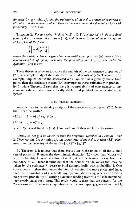
290 MICHAEL WOODFORD
for some O < q < minj qj*, and the trajectories of the o.d.e. system point inward at all points on the boundary of D. Then (n1, q,) -- I under the dynamics (2.4) with probability 1 as t -* oo.
THEOREM 2: For any point (nA, qA) E [n, n] X (O, lI], either (a) (n', q4) is a fixed point of the associated o. d.e. system (2.5), and the linearization of the o. d.e. system at (n, q) is of the form
[ .] = A [ ^] q - q
where the matrix A has no eigenvalues with positive real part; or (b) there exists a neighborhood N of (ni, q^) such that the probability that (n, q) -* N under the dynamics (2.4) is zero.
These theorems allow us to reduce the analysis of the convergence properties of (2.3) to a simple study of the stability of the fixed points of (2.5). Theorem 1, for example, implies that if the associated o.d.e. system has a globally stable fixed point, then the stochastic system (2.4) converges to those estimates with probabil- ity 1, while Theorem 2 says that there is no probability of convergence to any constant values that are not a locally stable fixed point of the associated o.d.e. system.
3. CONVERGENCE RESULTS
We now turn to the stability analysis of the associated o.d.e. system (2.5). Note that it can be written
(3.1a) nj = h (qj*lqj) Fj(n),
(3.1b) qj= qj* - qj,
where Fj(n) is defined by (1.5). Lemmas 1 and 2 then imply the following.
LEMMA 3: Let n, n be chosen to have the properties described in Lemmas 1 and 2. Then for any 0 < q < minj q *, the trajectories of the o.d.e. system (3.1) point inward on the boundary of the set D = [n, nh]m X [q, 1]m.
By Theorem 1, it follows that there exists a set I, the union of all the co-limit sets of points in D under the deterministic dynamics (2.5), such that (ne, q,) > I with probability 1. Whatever this set is like, it will be bounded away from the boundary of D. Hence it turns out that the bounds on the values that may be taken by the estimates hi cease to bind asymptotically with probability 1. One consequence is then that, under the kind of learning dynamics postulated here, there is no possibility of a self-fulfilling hyperinflation being generated; there is no positive probability of learning dynamics tending toward n = 0 (the nonmone- tary steady state) for t large. This result would suggest that the concern for the "tenuousness" of monetary equilibrium in the overlapping generations model,
This content downloaded from 128.59.154.119 on Mon, 25 Nov 2013 12:53:40 PMAll use subject to JSTOR Terms and Conditions

SUNSPOTS 291
that is often expressed (see, e.g., Wallace (1980)), because there is a continuum of hyperinflationary perfect foresight equilibria, is in fact unwarranted. In this respect our results support those of Lucas (1986).
Lucas' results are also corroborated by the following:
PROPOSITION 3: Suppose that m = 1, i.e., no sunspot variable is observed, and agents simply seek to learn the rate of return on money holdings (that, in this case, they presume to be constant). Then learning dynamics of the kind postulated here converge with probablity one to the monetary steady state, n = n*.
PROOF: In this case, q = 1 forever (since there is only one state). The system (3.1) reduces to
h = h [u'(n) - v'(n)].
By Assumptions (A.2)-(A.4), n = n* is a globally stable fixed point of this o.d.e. Then convergence of the learning process follows from Lemma 3 and Theorem 1.
In treating the case m > 1, we will assume the regularity condition:
(R) At each s.r.e.e. with n >> 0, no eigenvalue of DF has zero real part. Consequently, A(n) # 0.
It is evident that (R) will be satisfied for generic preferences; this will allow us to classify s.r.e.e. in terms of the sign of Ai(n) in certain results below.
Further immediate consequences of the form (3.1) are then the following:
LEMMA 4: Along any trajectory of the o.d.e. system (3.1), qj -qJ* as T -o 00.
Therefore (by Theorem 1) qjt -* qJ* with probability 1 under the stochastic dynamics (2.4) as t - oo0. Furthermore, the invariant set I is of the form J X { q* }, where J is the union of the w-limit sets of the points in [n, n]im under the o.d.e. system
(3.2) A 1 = h?(n).
LEMMA 5: For any point (n, q) e [n, n]m X (0, 1]m, there exists a neighborhood N of (ni, q) such that the probability that (ne, q,) -- N under the dynamics (2.4) is zero, unless q = q*, F(nf) = 0 (i.e., n is a s.r.e.e.), and DF(nf) has all eigenvalues with negative real part.
Lemma 5 follows from Theorem 2, because (3.1) implies that the matrix A referred to in Theorem 2, evaluated at a point (n', q*) where F(n') = 0, has the form
A= [DF(n) 2 ]
where Im is the m X m identity matrix. By the regularity assumption (R), DF(n) has no eigenvalues with positive real part if and only if all its eigenvalues have negative real part.
One case in which stronger conclusions are possible is the following.
This content downloaded from 128.59.154.119 on Mon, 25 Nov 2013 12:53:40 PMAll use subject to JSTOR Terms and Conditions
292 MICHAEL WOODFORD
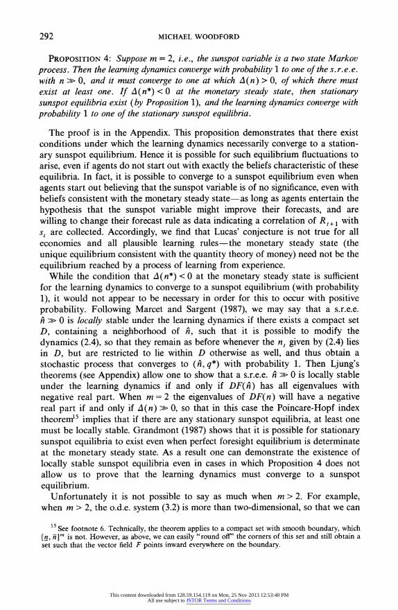
PROPOSITION 4: Suppose m = 2, i.e., the sunspot variable is a two state Markov process. Then the learning dynamics converge with probability 1 to one of the s. r. e. e. with n >> 0, and it must converge to one at which A (n) > 0, of which there must exist at least one. If A(n*) < 0 at the monetary steady state, then stationary sunspot equilibria exist (by Proposition 1), and the learning dynamics converge with probability 1 to one of the stationary sunspot equilibria.
The proof is in the Appendix. This proposition demonstrates that there exist conditions under which the learning dynamics necessarily converge to a station- ary sunspot equilibrium. Hence it is possible for such equilibrium fluctuations to arise, even if agents do not start out with exactly the beliefs characteristic of these equilibria. In fact, it is possible to converge to a sunspot equilibrium even when agents start out believing that the sunspot variable is of no significance, even with beliefs consistent with the monetary steady state-as long as agents entertain the hypothesis that the sunspot variable might improve their forecasts, and are willing to change their forecast rule as data indicating a correlation of Rt+1 with
st are collected. Accordingly, we find that Lucas' conjecture is not true for all economies and all plausible learning rules-the monetary steady state (the unique equilibrium consistent with the quantity theory of money) need not be the equilibrium reached by a process of learning from experience.
While the condition that A(n*) < 0 at the monetary steady state is sufficient for the learning dynamics to converge to a sunspot equilibrium (with probability 1), it would not appear to be necessary in order for this to occur with positive probability. Following Marcet and Sargent (1987), we may say that a s.r.e.e. n >> 0 is locally stable under the learning dynamics if there exists a compact set D, containing a neighborhood of n, such that it is possible to modify the dynamics (2.4), so that they remain as before whenever the n, given by (2.4) lies in D, but are restricted to lie within D otherwise as well, and thus obtain a stochastic process that converges to (f,q*) with probability 1. Then Ljung's theorems (see Appendix) allow one to show that a s.r.e.e. R ? 0 is locally stable under the learning dynamics if and only if DF(f) has all eigenvalues with negative real part. When m = 2 the eigenvalues of DF(n) will have a negative real part if and only if A (n) >> 0, so that in this case the Poincare-Hopf index theorem15 implies that if there are any stationary sunspot equilibria, at least one must be locally stable. Grandmont (1987) shows that it is possible for stationary sunspot equilibria to exist even when perfect foresight equilibrium is determinate at the monetary steady state. As a result one can demonstrate the existence of locally stable sunspot equilibria even in cases in which Proposition 4 does not allow us to prove that the learning dynamics must converge to a sunspot equilibrium.
Unfortunately it is not possible to say as much when m > 2. For example, when m > 2, the o.d.e. system (3.2) is more than two-dimensional, so that we can
15 See footnote 6. Technically, the theorem applies to a compact set with smooth boundary, which [n, n]m is not. However, as above, we can easily "round of' the corners of this set and still obtain a set such that the vector field F points inward everywhere on the boundary.
This content downloaded from 128.59.154.119 on Mon, 25 Nov 2013 12:53:40 PMAll use subject to JSTOR Terms and Conditions

SUNSPOTS 293
no longer use Bendixson's criterion to rule out closed orbits, as in the proof of Proposition 4. And when m > 2, an index of + 1 no longer still implies that all eigenvalues of DF(n) have negative real part. However, an index of -1 does imply that not all eigenvalues of DF(n) have negative real part, so that the s.r.e.e. must be unstable (by Theorem 2). Accordingly we have the following proposi- tion:
PROPOSITION 5: Let m be an arbitrary finite number of states. Then if A(n*) < 0 at the monetary steady state, the learning dynamics converge to that s.r.e.e. with probability zero. In particular, if perfect foresight equilibrium is indeterminate at the monetary steady state, there exists an open set of transition probability matrices
7Tjk for which the monetary steady state is unstable.
This result indicates that it is possible for the monetary steady state to be unstable for arbitrary m; but when m > 2 we do not then know that the learning dynamics converge to one of the stationary sunspot equilibria. Since o.d.e. system (3.2) might have a stable limit cycle or a chaotic attractor, we do not know that the learning dynamics need ever converge.
In Woodford (1987b), it is shown that for arbitrary m one can construct robust examples of economies in which the learning dynamics must converge to a stationary sunspot equilibrium, although no very general characterization is available in this case. The two-state sunspot processes to which Proposition 4 applies are degenerate cases of an m-state process, for any m > 2, and it can be shown that the o.d.e. system (3.2) for the degenerate m-state model is a Morse- Smale dynamical system (Palis (1969)); hence the global dynamics are struc- turally stable (Palis and Smale (1970)) under perturbations of the transition probability matrix away from the degenerate case.
4. ALTERNATIVE SPECIFICATIONS OF AGENTS' INFORMATION
The above analysis (especially Proposition 4) indicates conditions under which the learning dynamics converge with probability 1 to one of a small set of stationary sunspot equilibria. However, in reaching this result we have assumed that all agents observe a particular sunspot variable, and sort their observations of (Rt+,, et) on the basis of it, and that no agents sort their observations on the basis of any other random variable. In fact, our stability results are quite sensitive to variations in the specification of the variables that agents use in their forecasts. In this section, we briefly consider two extensions of the model of Section 2-allowing agents to use additional sunspot variables in their forecasts, and allowing different agents to use different variables.
The demonstration that a given s.r.e.e. is locally stable when all agents use in their forecasts only the most recent observation of a single sunspot variable st, does not mean that the mere fact that all agents observe st suffices to insure that this s.r.e.e. is locally stable and hence a possible outcome of the learning dynamics. For if agents begin to use in their forecasts some other random
This content downloaded from 128.59.154.119 on Mon, 25 Nov 2013 12:53:40 PMAll use subject to JSTOR Terms and Conditions
294 MICHAEL WOODFORD
variable as well, even one that is distributed completely independently of st, the local stability of the s.r.e.e. in question may be reversed. A simple example of how this can occur is provided by the contrast between Propositions 3 and 4 of Section 3; use of an additional variable in forecasting (the case of Proposition 4) can render unstable an equilibrium (the monetary steady state) that would be stable if that variable were ignored (as in the case of Proposition 3).
Evans (1987) proposes a distinction between "weak" and "strong" expecta- tional stability that we may adapt to the present context. A s.r.e.e. will be said to be weakly stable if it is locally stable under the sort of learning dynamics modeled in Section 2, when agents use in their forecasts only the random variables which affect the equilibrium choice of nt in the s.r.e.e. in question (i.e., the minimum information set consistent with that equilibrium). It will be said to be strongly stable, though, only if it continues to be locally stable when agents also use some other finite-state Markov variable, independent of the variables in the minimum information set, regardless of what the stochastic properties (i.e., transition probability matrix) of the additional variable might be. Under this terminology, the monetary steady state is always weakly stable, by Proposition 3, but may not be strongly stable, by Proposition 4.
The following result establishes a case in which the monetary steady state is strongly stable.
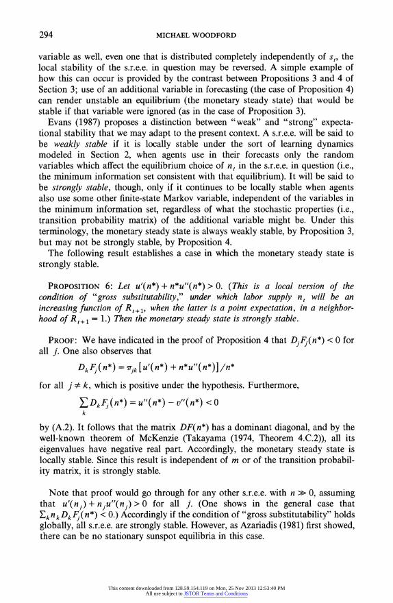
PROPOSITION 6: Let u'(n*) + n*u"(n*) > 0. (This is a local version of the condition of "gross substitutability," under which labor supply nt will be an increasing function of Rt+1, when the latter is a point expectation, in a neighbor- hood of Rt+1 = 1.) Then the monetary steady state is strongly stable.
PROOF: We have indicated in the proof of Proposition 4 that DjFj(n*) < 0 for all j. One also observes that
DkFj(n*) = g7jk [ u'(n*) + n*u"(n*)] /n*
for all j ' k, which is positive under the hypothesis. Furthermore,
EDkFj(n*) = u"(n*) - v"(n*) < 0 k
by (A.2). It follows that the matrix DF(n*) has a dominant diagonal, and by the well-known theorem of McKenzie (Takayama (1974, Theorem 4.C.2)), all its eigenvalues have negative real part. Accordingly, the monetary steady state is locally stable. Since this result is independent of m or of the transition probabil- ity matrix, it is strongly stable.
Note that proof would go through for any other s.r.e.e. with n >> 0, assuming that u'(nj) + nju"(nj) > 0 for all j. (One shows in the general case that EknkDkFj(n*) < 0.) Accordingly if the condition of "gross substitutability" holds globally, all s.r.e.e. are strongly stable. However, as Azariadis (1981) first showed, there can be no stationary sunspot equilibria in this case.
This content downloaded from 128.59.154.119 on Mon, 25 Nov 2013 12:53:40 PMAll use subject to JSTOR Terms and Conditions

SUNSPOTS 295
It is not known whether stationary sunspot equilibria can ever be strongly stable, although it is easy to construct examples showing that they need not be (see Woodford (1987b)). Evans (1987) shows that for a particular parametric class of utility functions, it is impossible for two-state stationary sunspot equilib- ria to be "strongly expectationally stable." However, his "expectational stability" criterion, while related to local stability under the learning dynamics treated here,'6 is not an identical criterion, so that his proof does not work for our case. (Nor does it work, even for his stability criterion, outside his special class of utility functions.) In particular, Evans shows that in his case a two-state sunspot equilibrium is always unstable when an additional independent two-state sunspot variable is introduced, with transition probability matrix Pjk close enough to Pll = P22= 0, P12 = P21 = 1. But it is shown in Woodford (1987b) that one can easily construct counterexamples to this latter proposition, in the case of our own explicit learning dynamics.
But even if Evans' instability thesis were correct in our case, this would not be a reason to suppose that the monetary steady state is in some sense more " robust" in general than are the sunspot equilibria. For if it were indeed true that no sunspot equilibria were ever strongly stable, then when A(n*) < 0, one would have to conclude that no s.r.e.e. are strongly stable. Hence it would not be sensible to propose that only strongly stable equilibria should be regarded as possible outcomes of the learning process.
What the foregoing discussion does clearly indicate is that the conditions for instability presented in Section 3 represent more robust results than the condi- tions presented under which equilibria are stable. For an instability result can never be overturned by supposing that agents use some additional, independent random variable in their forecasts.
PROPOSITION 7: Let r, and st be two independent finite-state (p-state and m-state respectively) sunspot variables, and let n be a stationary sunspot equilibrium in which output nt depends upon st only. Suppose that n is unstable under the learning dynamics when agents use only st in their forecasts. Then the sanme equilibrium is also unstable when agents use both rt and st in their forecasts.
PROOF: Let rt have transition matrix Pab, a, b = 1,..., p, and st have transi- tion matrix '7jkI j, k = 1,..., m. Let aj denote the overall state in which rt = a, St= j. Then at the equilibrium n, when agents use both rt and st in their forecasts, the mp x mp matrix DF has the form
DajFaj = Paa7TjknjU n j),
DbkFaj Pab'Tjkl IUk, if bk # aj,
where Uj = u'(nj) + nju"(nj), Vj = v'(nj) + njv"(nj).
16 For further discussion of the relationship, see Woodford (1986a).
This content downloaded from 128.59.154.119 on Mon, 25 Nov 2013 12:53:40 PMAll use subject to JSTOR Terms and Conditions

296 MICHAEL WOODFORD
Now suppose that e E Rm is an eigenvector of DF when only s, is used, with eigenvalue X. Then
gkUkek,= (Vj+ Xnj)ej k
for j= 1,..., m. It follows that the mp-vector e defined by eaj = e1 is an eigenvector of DF when both r, and s, are used, again with eigenvalue X, since
E 2 DbFJbkFaj1bk [J [ Pab7TjkUkek 1Vjej b k b k
=Xej =Xe aj
Hence all m eigenvectors of DF in the former case are also among the mp eigenvectors of DF in the latter case. If the equilibrium is unstable in the former case, at least one eigenvalue has positive real part, and so at least one has positive real part in the latter case as well, making the equilibrium again unstable.
Hence, for example, the conclusion that the monetary steady state is unstable when A(n*) < 0 remains robust under the addition to agents' information set of additional independent sunspot variables.
Our results in Section 3 also depend upon an assumption that all agents are attempting to learn the significance of the same m-state sunspot variable. An obvious question is the robustness of our conclusions to various sorts of hetero- geneity in agents' information sets (or their maintained hypotheses about what variables might matter). We first consider the case in which only a fraction a of the population use the sunspot variable in forecasting. The remaining agents also use a Robbins-Monro algorithm to estimate their optimal labor supply, but under a maintained hypothesis that (R,+?, -,) are always drawn from the same distribu- tion G, regardless of the current sunspot state. Obviously, when a < 1 the economy cannot ever get to a sunspot equilibrium of the kind described in Section 1, although it might converge to a pseudo-equilibrium in which the action of the nonsunspot watchers is optimal subject to the constraint that they not act differently in the different sunspot states. One can, however, consider the stability of the monetary steady state under learning dynamics of this sort. As one might expect, a smaller fraction a of sunspot watchers makes it harder for a belief in sunspots on the part of those agents to become self-fulfilling.
PROPOSITION 8: Consider an economy in which only a fraction a of the popula- tion are sunspot watchers, as described above. Then for any given specification of preferences, there exists a fraction a* > 0 such that if a < a*, the monetary steady state is stable.
This content downloaded from 128.59.154.119 on Mon, 25 Nov 2013 12:53:40 PMAll use subject to JSTOR Terms and Conditions

SUNSPOTS 297
PROOF: The o.d.e. system corresponding to (3.2) in this case is
41a -hF_Tjk "ank+ a)N U (ank+(1-a)N j , ()
k ank? (1 -a)N un'k I a N ) (4.1b) 1i= h Tjk ank +(1- a)N Ul ank+(l-a)N N vfN
(= k (an + (1-a)N an1 + (1-a)N
where n1 is the sunspot-watchers' estimate of the optimal labor supply in sunspot state j, N is the sunspot-ignorers' estimate of the optimal labor supply. Lineariz- ing around the monetary steady state (n1 = = nm = N = n*), (4.1) becomes
(4.2 [ hB C][N-n*]
where
A = aDF(n*) + (1-a)CI,
C = uff(n*) - v'(n*).
The eigenvalues of the matrix in (4.2) are accordingly C and the m quantities aX + (1 - a)C where A (i =,...,m) are the eigenvalues of DF(n*). Since C < 0 (by (A.2)), it follows that whatever the eigenvalues of DF(n*) might be, there exists an a* > 0 such that the monetary steady state is locally stable for all a < a*.
This result indicates that Proposition 4 only provides a cogent explanation of how an economy could diverge from the monetary steady state, and end up in a sunspot equilibrium, insofar as there is a sunspot variable that one can reason- ably expect a large fraction of the population to consider potentially useful for forecasting purposes. One possibility would be if a sufficiently striking accidental correlation between fluctuations in asset returns (due, perhaps, to fundamental shocks that are not observable to a large number of agents) and a particular sunspot variable happened to occur, which, once noticed and publicized, led to a large number of agents' using that variable in their forecasts, so that the correlation came to be perpetuated (and rendered nonaccidental).
Perhaps a more interesting possibility would be an interpretation of the variable st as in fact a small shock to fundamentals, so that agents would necessarily be led to use it in their forecasts. Under the same circumstances under which the Azariadis model has stationary sunspot equilibria, introduction of a very small shock to fundamentals (with the same stochastic properties as the sunspot variable considered previously) will result in the existence of multiple s.r.e.e. in which output responds only to the fundamental shock."7 In one of these (a small perturbation of the former monetary steady state), the response to the
17 See Woodford (1986b, Theorem 2).
This content downloaded from 128.59.154.119 on Mon, 25 Nov 2013 12:53:40 PMAll use subject to JSTOR Terms and Conditions

298 MICHAEL WOODFORD
shock is similarly small, but in others (perturbations of the former sunspot equilibria) the response to the shock is much larger than the shock itself. In equilibria of the latter sort, the fluctuations in output are effectively due to self-fulfilling expectations, rather than the changes in fundamentals-the shock to fundamentals acts like a sunspot variable, cuing shifts in agents' expectations. If one supposes that agents must learn how much to change their forecasts in response to the shock, through a learning process of the kind modeled above, one finds that under the same conditions under which the monetary steady state is unstable in the pure sunspot case, the small-response equilibrium will be unsta- ble; and under the same conditions under which one or more sunspot equilibria are stable, one or more of the large-response equilibria will be stable.
5. CONCLUSION
Our results indicate that one of Lucas' (1986) conjectures is not always correct: a plausible learning process need not always converge to the quantity-theoretic equilibrium, the monetary steady state. This point can be sharpened by consider- ing an economy in which the Markov process st represents the stochastic rate of growth of the money supply between periods t - 1 and t, where new money is paid out in proportion to existing money holdings. There will still be a s.r.e.e. in which Rt+I is always equal to 1, and this will be the quantity-theoretic equilib- rium, in which the rate of growth of money prices between t -1 and t will always exactly equal the rate of growth of the money supply. But corresponding to the stationary sunspot equilibria discussed above, there will now be s.r.e.e. in which different realizations of the rate of growth of the money supply correspond to different levels of output, and in which the rate of inflation will not always equal the rate of growth of the money supply.18 Equations (2.4) still describe the learning dynamics in this case, and so the results of Section 3 give conditions under which the learning dynamics converge to one of the non-quantity-theoretic equilibria.
Our results are contrary to the spirit of Lucas' remarks in a deeper sense as well. Lucas proposes that the analysis of learning processes may allow one to solve the challenge posed to the predictive claims of economic theory by large multiplicities of rational expectations equilibria in models such as the overlap- ping generations model, by allowing one to pick out a single equilibrium as the one to which a reasonable learning process should converge. Our results, how- ever, do not suggest that it will always be easy to single out a single equilibria on such grounds.
This does not, however, mean that such a model implies no testable predictions about the long run state of the economy. Nontrivial restrictions upon the data are implied by all s.r.e.e. of a given model.9 And while our formal results provide no general demonstration that learning must eventually converge to a s.r.e.e., they
18 See Farmer and Woodford (1984), and Woodford (1986, Section 4). 19 See Woodford (1987b, Section 4).
This content downloaded from 128.59.154.119 on Mon, 25 Nov 2013 12:53:40 PMAll use subject to JSTOR Terms and Conditions
SUNSPOTS 299
cast no doubt upon such a presumption. Finally, a theory that identifies the situations in which sunspot equilibria are or are not possible can be of use, without having to be able to predict that one of the many possible equilibria must occur. One may, for example, be interested in the design of policy regimes that are not subject to the sort of endogenous instability represented by the existence of sunspot equilibria, as argued in Woodford (1987a).
Dept. of Economics, University of Chicago, 1126 East 59th Street, Chicago, IL 60637, U.S.A.
Manuscript received July, 1985; final revision received March, 1989.
APPENDIX
PROOF OF THEOREM 1: Theorem 1 is a straightforward application of a theorem due to Ljung (1975, 1977). We restate Ljung's theorem here, in the form that we make use of, because it is not well-known among economists. In particular, we require a less restrictive version of the theorem than is used by Marcet and Sargent (1986, 1987).
Consider a recursive algorithm of the form
(a.1) xt = Xt_ 1 + t-1Q (Xt- 1, Zt),
(a.2) = =A(x, )z,1 + B(xt_ )e,
where x, is an n-vector of estimates, zt is an m-vector of additional state variables, e, is a p-vector of exogenous random shocks, Q is a vector-valued function, and A and B are matrix-valued functions. We make the following assumptions on the form of the algorithm. (In each case, DR is some open, connected subset of R,, in which the assumptions are valid.)
(R.1) Ie,I is bounded with probability 1 for all t.
(R.2) A (x) has all eigenvalues strictly inside the unit circle, for all x E DR.
(R.3) A and B are Lipschitz continuous functions of x, i.e., there exists a finite constant C such that IA(xl) - A(x2)1 < Clxl - x21, for xl, x2 E DR, and analogously for B. Furthermore, B(x) is bounded for all x E DR.
Note that (R.1)-(R.3) imply the existence of a bounded invariant set DZ C R', such that zo E DZ implies zt E D. for all t, with probability 1. We also assume the following.
(R.4) Q is a Cl function of x and z, and its derivatives are bounded, for all x E DR and z E D.
(R.5) For x E DR, define the sequence of random variables {2,(x1)} by zt(x) =A(x1)it_(x) + BF (x) et; zo (3c) = O-
(In other words, this is what the evolution of zt would be, by (a.2), if x, were to remain fixed at x.) Then the limit
f (X-)-= lim Eo Q (X-) it(x t __ 0
exists for all x- E DR, where Eo denotes the expectation prior to the realization of any of the random shocks { el, e2, ... }. Furthermore
limt Q1 , fr l (x)) = (x) t ? ?? S=1 with probability 1, for all xc E- DR.
This content downloaded from 128.59.154.119 on Mon, 25 Nov 2013 12:53:40 PMAll use subject to JSTOR Terms and Conditions

300 MICHAEL WOODFORD
Assumptions (R.1)-(R.5) are stronger than, but suffice to imply, the "assumptions III" of Ljung (1975) (or equivalently, the "assumptions C" of Ljung (1977)). In particular, (R.2) is an unnumbered assumption made by Ljung; Ljung's III.1 is implied by (R.4); III.2 is part of (R.3); III.3 is part of (R.5); III.4 is implied by the boundedness assumptions of (R.1), (R.3), and (R.4); and III.5 and III.6 are implied by the special form we have written for (a.l).
Ljung proves the following theorem:
THEOREM Al: Consider an algorithm of the form (a.l)-(a.2), and suppose that it satisfies (R.1)-(R.5). Assume furthermore that (i) there is a compact set D1 c DR such that xt E D1 infinitely often with probability 1; (ii) the o.d.e. system
(a.3) x =f (x)
has an invariantt set I whose domain of attraction includes all of D/. Then xt - I with probability 1 as t - oo.
This is Corollary 1 to Theorem 1 of Ljung (1975), or Theorem 1 of Ljung (1977). The application to algorithm (2.4) is as follows. Here x, = (ni,, q,), a 2m-vector (of which one
element of q, is redundant), zt = (fi, ii, - _1, E (st-1)), and e, = (e,1, 4(s,), '(st,_)). In writing the above we use the notation
nt=E nl,_ AJ (st )
for the level of output actually supplied in period t. We can choose DR to be any open connected set such that
[ "I
n x [q,i] c DR C DKC (0, n) X R+x +
where q is some quantity 0 < q < mn q., and DK is some compact set. Since we have assumed that ?, has bounded support, and 4i(s,) tal?es on only m different values, (R.1) is satisfied.
The matrices A and B are in this case:
O O0 O O0 n,1 01
Al=I o o o0 B(xt-1)= 0 0 0 g j' [1 g oj
O0 O O O- 0 O Ij
Since all eigenvalues of A are zero, (R.2) and (R.3) are satisfied. The set DZ can be chosen to be N2 X supp H X M where
N = { n E R"3q E R" such that (n, q) E DR}
and M is the finite set of values that 4(s,) can take. Let us neglect for the moment the bounds (n, -n) in (2.4). Then the vector function Q is (Q1, Q2),
where
Ql (x, zt) =hq, 1[(fin/i1t-)u'(ht) - v'(n.) - 1- J(St-,),
Q2 (x, zt) =
y (St_ 1) -qJ.
Given that in,t and ql are bounded away from zero, that ii is bounded away from n, and Assumption (A.1) on u and v, assumption (R.4) is satisfied.
In this case, for any x- E DR, we can write
Q( , M,()) = t ( + M2t C et- 1
where Mlt and M2, are finite state Markov processes, independent of the { ,} process. (We will similarly write M2t(x)' in the case of the decomposition of Ql, etc.) By independence, we can write EO[Q(x, z,(x))] = E0[ Ml,(x)], and then by a familiar property of finite state Markov processes (Doob
This content downloaded from 128.59.154.119 on Mon, 25 Nov 2013 12:53:40 PMAll use subject to JSTOR Terms and Conditions

SUNSPOTS 301
(1953), pp. 173-174), the limit of this expression as t -+ oo exists and is equal to (f1(x), f2(x)) where
f, ( J/J)[EnXk ( nkln U ( nk )V ( n
fJ2(X) =q7l _q,.
Furthermore, by the strong law of large numbers for finite state Markov processes (Doob (1953), p. 219)),
iim t-l ml M(x) =f(x) t + ?0
with probability 1. We can also write
(a.4) X J 1 ( /J ( r-I ) r=1 n=L r=_
where each E' is the value of et_ in the nth period t such that 4J((sr ) =j, and -(t) is the number of such periods up through period t, i.e.,
T(t) = E 4'(Sr-1) r=1I
Now of the three terms on the right-hand side of (a.4), the first is a constant (that depends upon x), the second is a sum of independently and identically distributed (i.i.d.) random variables with mean zero, and the third is a sum of variables that form a finite state Markov process. By the law of large numbers for i.i.d. random variables (Doob (1953), pp. 142, 145), the second term converges to zero with probability 1 as t -- oo, while by the law of large numbers for finite state Markov processes cited above, the third term converges to qJ* with probability 1. Hence expression (a.4) converges to zero with probability 1 as t -. oo. Since M2t(x)j = 0 for all j, these components of t r. 1M2r(-),r are zero for all t. Hence
iim t - lE Q(x Zr() f CO t >?? r=1
with probability 1, and condition (R.5) is satisfied. Theorem Al then implies Theorem 1, if it can be shown that x, enters the set D - [n, n]m X [q, 1]m
infinitely often with probability 1. By the law of large numbers for a finite state Markov process, qt . q* with probability 1. Hence qt E=- [q, i]tm infinitely often, with probability 1. It remains only to show that n, enters [n, i]n" infinitely often. But this is guaranteed by our assumption that (because of their maintained hypothesis) agents never allow the estimates hlt to leave the interval [n, n]. Ljung (1975, Theorem 3 and discussion, or 1977, Theorem 4 and discussion) shows that one can insure the "boundedness condition" needed for Theorem Al by a modification of the algorithm (a.1) of this sort, with the qualification that, in order to rule out an accumulation point on the boundary of the set D, one must show that the trajectories of the o.d.e. system (a.3) point inward at all points on the boundary. The latter condition is part of the hypothesis of Theorem 1 stated in the text.
Although we will not discuss the generalization here, it is worth noting that Ljung states Theorem Al for the case of algorithms in which the vector function Q may be time-varying. This extension would be necessary if we were to replace the qjtll in (2.4b) with q71 (which would be the straightforward application of (2.2), since qt, is a time varying function of (x,-1, zt)). Similarly, if we were to assume that agents choose n, using the estimates n, that take into account the observation (R,, e,1)-instead of continuing to use n,-1-we would find that, in the case that s, =St =
j, t (1J, - h1j_- ) would be a time-varying function of (x,-1, z,). Ljung's theorem is general enough to handle these cases as well, and in fact one finds that neither modification has any effect upon the asymptotic dynamics.
This content downloaded from 128.59.154.119 on Mon, 25 Nov 2013 12:53:40 PMAll use subject to JSTOR Terms and Conditions

302 MICHAEL WOODFORD
PROOF OF THEOREM 2: Ljung also shows the following.
THEOREM A2: Consider an algorithm of the form (a.1)-(a.2), and suppose that it satisfies (R.1)-(R.5). Then suppose that x* E DR is such that for an arbitrary neighborhood N of x*, the probability that x, -+ N is positive. Then f (x*) = O.
This is Theorem 4 of Ljung (1975), stated under more restrictive assumptions as part of Theorem 2 of Ljung (1977). Since the "assumptions III" of Ljung (1975) suffice, our assumptions (R.1)-(R.5) suffice as well. Application to the algorithm (2.4), as in the proof of Theorem 1 above, gives half of Theorem 2.
We now impose additional assumptions upon the general class of recursive algorithms under consideration.
(R.6) For any x E DR such that f (x) = 0, Eo[Q(x, z,(x))] is C' for x in a neighborhood of x, and the derivatives converge uniformly in this neighborhood as t -+ oo.
(R.7) For any x E DR such that f(x) = 0, and any left eigenvector v of Df(x-) whose eigenvalue has positive real part, there exists a constant C > 0 such that for any sequence of positive constants { y, }, and any M > N,
M 2 M
(.)Eo 1 yt,vQ((x~), z,(x~)) > CIV12 E t2.
t =N t =N
Following Ljung, one can then show the following.
THEOREM A3: Consider an algorithm of the form (a.1)-(a.2), and suppose that it satisfies (R.1)-( R.7). Then suppose x* E DR is such that for an arbitrary neighborhood N of x*, the probability that xt -+ N is positive. Then Df (x*) has no eigenvalues with positive real part.
This corresponds to Theorem 5 of Ljung (1975), or equivalently to part of Theorem 2 of Ljung (1977). Ljung's statement of the theorem, however, assumes a stronger restriction upon the algorithm than does ours. For Ljung assumes, in addition to (R.6) and a condition related to (R.7), that his "assumptions I or II" (the "assumptions A or B" of Ljung (1977)) are satisfied. Our assumptions (R.1)-(R.5) imply all of the "assumptions I" of Ljung (1975), except I.1, the assumption that { e, } is i.i.d. In our case, the { 4i(s,)} are not independently distributed. However, examination of the proof of Theorem 5 given in Ljung (1975) shows that the version of (R.7) given here suffices to allow proof of Ljung's Lemma D.1, even without the assumption that {e,} is i.i.d. And the assumption of independence is used nowhere else in the Proof of Theorem 5. (See also the remark about generalization of Theorem 5 in Appendix G of Ljung (1975).)
The algorithm (2.4) is easily shown to satisfy (R.6) and (R.7). Since for any x e DR, Q(x, z,(x)) is a finite state Markov process, with the transition probabilities between the states independent of x, we can write
EQ[ Q( x, z, (x))] = PjQj (x)
where Pj, represents the probability of being in state j in period t. This expression is C' in x because each of the time-invariant functions Qj (x) is C1, and its derivatives E P, DQ1 (x) converge uniformly in a neighborhood of any x E DR, because DQj(x) is continuous and Pji converges. Thus (R.6) is satisfied.
In the case of algorithm (2.4), f(x) = 0 implies that x has the form (n?, q*), for some n? E [n, ii]". Furthermore, at any such point, Df (x) is block-diagonal, since f'(no, q) = 0 independently of q and f 2(n, q*) = 0 independently of n. Hence the left eigenvectors of Df(x) are either of the form (vl, 0), where v, is a left eigenvector of DIf', or of the form (0, v2), where v2 is a left eigenvector of D2f 2. Since D2 f 2 = - I., all eigenvectors of the latter sort have eigenvalue - 1. Hence we need only verify inequality (b.1) for an arbitrary nonzero vector of the form (v,,0).
This content downloaded from 128.59.154.119 on Mon, 25 Nov 2013 12:53:40 PMAll use subject to JSTOR Terms and Conditions

SUNSPOTS 303
In this case, at a point x = (no, q*),
M 2
Eo E -y, Q( x, z, ( x) t=N
2 M Eo 7E v (y 1 ) hq* E( n) -Et I
t=N k k
M 2 t=N k
M 2
Eo E -yt2E vj0| tj)q- E noln u'( no, 1k (St) - vE- no
t=N
= ( y2) h2a2Zvl1j.
t=N
HIere we have used the fact that the variables { E,}are independent of one another and of the variables { s, }. This establishes (b.l), where CIvI2 = h 2JlJ oethat this formula implies a finite constant C regardless of the metric used for 1v12. Hence (R.7) is satisfied as well. Theorem A2 then implies the part of Theorem 2 that remained to be proved.
Note the role in this last part of the proof of the assumption that there exist the taste shocks { Et } even though the variance of these shocks may be arbitrarily small. In the absence of the taste shocks, in the case of the monetary steady state, x = (n*, q*), one would have Q(x, z,x) = 0 for all possible sunspo)t histories, so that (R.7) would not be satisfied, if in fact (as is shown in the text to be possible) there should exist an eigenvalue of Df(x) with positive real part.
CONVERGENCE OF THE ROBBINS-MONRO ALGORITHM
It is asserted in the text that, if agents' maintained hypothesis were true, the estimator (2.3) would converge with probability 1 to the true value n1. This is a simple application of Theorem Al used above to prove Theorem 1. In this case x, = h11, and z, = e,= (R,, e,i1). We can choose DR to be any open interval containing [_, ni], and bounded away from both 0 and n.
Since, according to agents' maintained hypothesis, both CJand H1 have bounded support, (R.1) is satisfied. The matrix A is made up entirely of zeroes, while B is the identity matrix. Since both are constant, and all eigenvalues of A are zero, (R.2) and (R.3) are satisfied. The set Dz can be chosen to be supp G1 X supp HJ.
The function Q is
Since CJis bounded both above and away from zero, and DR is bounded away from ni, Assumptions (Al1) imply that (R.4) is satisfied. Finally, since according to agents' maintained hypothesis, z, is identically and independently distributed,
-r Cr 1 rEV oeta hsfruaipisafnt
This content downloaded from 128.59.154.119 on Mon, 25 Nov 2013 12:53:40 PMAll use subject to JSTOR Terms and Conditions

304 MICHAEL WOODFORD
is independent of t, and, by the law of large numbers for i.i.d. variables (Doob (1953, p. 142)),
rim t- I E Q(x, it () =f (X) t- ?o s=1
with probability 1. Hence (R.5) is satisfied as well, and Theorem Al applies. Now Q is a strictly decreasing function of nj, so f (nj) must be as well. Then f has a unique zero
at n1. (Note that f (n.) = 0 is just the first order condition for optimal labor supply in sunspot state j.) The o.d.e. (a.3) has trajectories pointing inward at the boundaries of the interval [, -n], and the domain of attraction of the fixed point n1 includes all of [n, -n]. Hence nj - n1 with probability 1.
For further discussion of the convergence of algorithms of this type, see Ljung and Soderstrom (1983).
PROOF OF PROPOSITION 4: We will make use of the following extension of the familiar Poincare- Bendixson Theorem for two-dimensional flows (Sansone and Conti (1964, Theorem IV.4)).
LEMMA 6: Consider a C1 o. d.e. system defined on a compact subset D of R2, such that trajectories point inward everywhere on the boundary of D, and suppose that all fixed points of the o. d.e. system are hyperbolic. Suppose also that no w-limit set of any trajectory in D contains a Jordan curve. Then every trajectory in D converges to a fixed point.
PROOF OF THE LEMMA: The assumption that all fixed points are hyperbolic implies, by the inverse function theorem, that each is locally unique. This implies, by a standard argument (see, e.g., Mas-Colell (1985), Proposition 5.5.2), that the fixed points in D are finite in number. Then by Theorem VII.4.2 of Hartman (1973), the w-limit set of any trajectory y(t) in D consists either of a fixed point, a closed orbit, or of a finite set of fixed points {xi } and a finite or infinite set of trajectories { yj }, such that for each j, yj does not pass through a fixed point, but converges to one of the fixed points xi as t -+ oo and also to one of them as t -+ - oo. The case of a closed orbit is ruled out by hypothesis. We wish to show that in the third case as well, there must exist a Jordan curve as part of the limit set. Then the limit set must be a fixed point.
We argue as follows. If the limit set contains more than one fixed point, it must contain at least one trajectory Yl, since the limit set must be connected. This trajectory Yl converges to a fixed point xl as t -. oo. If Yl also converges to xl as t -+ oo, we have established the existence of a Jordan curve. Suppose not. Then let B be the closure of a ball around xl, chosen to be small enough that it does not contain all of Yl, and such that Yl enters the ball at only one point. (Because of the hyperbolicity of xl, a small enough ball must have this property.)
Since xl belongs to the w-limit set of Yl, there must exist a sequence of times { t" } such that y(t") -. xl as n -. oo. There will also exist some N such that y(t") e B for all n > N. But since the w-limit set also includes points outside of B, the trajectory y(t) must leave B infinitely often. For each n > N, let t' denote the first time after t, that the trajectory leaves B. Then for each n > N, y( t') lies on the boundary of B, at a point at which the trajectories of the o.d.e. system point outward. Since y(t.) converges, y(t') must converge as well, to some point
- on the boundary of B, and the
trajectory of the o.d.e. system passing through -
must either point outward or be tangent to the boundary. This point y must also belong to the w-limit set, but it cannot be part of y,, nor even part of the stable manifold of xl.
Since such a point exists, no matter how small the ball B is made, there must exist as part of the limit set another trajectory Y2 that approaches xl as a limit point. Trajectory Y2 cannot be part of the stable manifold of xl, and hence must be part of the unstable manifold. By the Hartman lemma cited above, Y2 must converge to one of the fixed points xi as t -+ oo; let that fixed point be X2. If x2 = xl, we have proved the existence of a Jordan curve, made up of the trajectory Y2 and the point xl. Likewise, if x2 is the point to which Yl converges as t -+ oo, we have proved the existence of a Jordan curve, made up of Yl, Y2, xl, and x2.
Suppose neither is the case. Then we can repeat the above reasoning at point x2, and so show the existence, as part of the limit set, of another trajectory y3, belonging to the unstable manifold of x2. This trajectory converges to some fixed point x3 as t -+ oo. Continuing this reasoning, since the number of fixed points in D is finite, we eventually must show the existence of a Jordan curve. Since all the fixed points are hyperbolic, the trajectories connecting them all form parts of the stable and unstable manifolds of each fixed point, and the Jordan curve is piecewise smooth. There is
This content downloaded from 128.59.154.119 on Mon, 25 Nov 2013 12:53:40 PMAll use subject to JSTOR Terms and Conditions

SUNSPOTS 305
accordingly no difficulty in defining the line integral used in the proof of Bendixson's criterion.
PROOF OF PROPOSITION 4: By Theorem 1 and Lemma 3, the learning dynamics converge with probability 1 to set I, as noted earlier, and by Lemma 4, I = J X { q*}. We wish to determine the elements of J. We first observe that
(c.l) Dj Fj ( n) = q7r, u"( nj )- E: s7k n k ul( n k )nj - v"( nj) < G k*j
at any point n >> 0, because of (A.2). It follows that the divergence D1 F1 + D2 F2 is negative at all points in [n, n-]2, and hence, by Bendixson's criterion (Sansone and Conti (1964, Theorem IV.21)), the o.d.e. system (3.2) cannot have any closed orbits. (We use here again Lemma 3.) From the proof given by Sansone and Conti it is evident that the same criterion in fact rules out any Jordan curve that is a union of trajectories and hyperbolic fixed points, since the same line integral could be defined and would have to vanish in that case as well.2
Lemma 6 applies to our case because (R) implies that the fixed points of (3.2) are hyperbolic. Since in our case there can be no Jordan curve made up of trajectories, no w-limit set can contain a Jordan curve. Lemma 6 then implies that J consists solely of fixed points. It then follows from Lemma 5 that there is probability zero of converging to any s.r.e.e. unless DF(n) has both eigenvalues with negative real parts. But by (c.1), the trace of DF(n) must be negative, so that at least one eigenvalue has negative real part. Hence both eigenvalues have negative real parts if and only if A(n) > 0.
REFERENCES
AZARIADIS, C. (1981): "Self-fulfilling Prophecies," Journal of Economic Theory, 25, 380-396. AZARIADIS, C., AND R. GUESNERIE (1982): "Propheties Creatrices et Persistance des Theories," Revue
Economique, 33, 787-806. (1986): "Sunspots and Cycles," Review of Economic Studies, 53, 725-738.
BLACK, F. (1974): "Uniqueness of the Price Level in Monetary Growth Models with Rational Expectations," Journal of Economic Theory, 7, 53-65.
BRAY, M. M. (1982): "Learning Estimation and the Stability of Rational Expectations," Journal of Economic Theory, 26, 318-339.
(1983): "Convergence to Rational Expectations Equilibrium," in Individual Forecasting and Aggregate Outcomes, ed. by R. Frydman and E. S. Phelps. Cambridge: Cambridge Univ. Press.
BRAY, M. M., AND D. M. KRuEPs (1987): "Rational Learning and Rational Expectations," in Arrow and the Ascent of Modern Economic Theory, ed. by. G. R. Feiwel. New York: NYU Press.
BRAY, M. M., AND N. E. SAVIN (1984): "Rational Expectations Equilibria, Learning, and Model Specification," Economic Theory Disc. Paper No. 79, Cambridge Univ.
CASS, D., AND K. SHELL (1983): "Do Sunspots Matter?" Journal of Political Economy, 91, 193-227. CHIAPPORI, P.-A., AND R. GUESNERIE (1989): "On Stationary Sunspot Equilibria of Order k," in
W. A. Barnett, J. Geweke, and K. Shell, eds., Economic Complexity: Chaos, Sunspots, Bubbles, and Nonlinearity. Cambridge: Cambridge University Press.
CYERT, R. M., AND M. H. DEGROOT (1974): Rational Expectations and Bayesian Analysis," Journal of Political Economy, 82, 521-536.
DOOB, J. L. (1953): Stochastic Processes. New York: Wiley. EVANS, G. (1987): "The Fragility of Sunspots and Bubbles," I.M.S.S.S. Tech. Rep. No. 514, Stanford
Univ. FARMER, R. E. A., AND M. WOODFORD (1984): "Self-fulfilling Prophecies and the Business Cycle,"
CARESS W.P. No. 84-12, Univ. Pennsylvania. FUCHS, G. (1979a): "Are Error Learning Behaviors Stabilizing?" Journal of Economic Theory, 3,
300-317. (1979b): "Dynamics of Expectations in Temporary General Equilibrium Theory," Journal of
Mathematical Economics, 6, 229-252.
20 Strictly speaking, Green's theorem requires that y be a smooth curve. But in the case of a limit set containing a Jordan curve y that is not smooth at all points (e.g., at points where two trajectories each approach a fixed point), we could still obtain the contradiction by applying Green's theorem to a nearby curve in which the corners have been "rounded off."
This content downloaded from 128.59.154.119 on Mon, 25 Nov 2013 12:53:40 PMAll use subject to JSTOR Terms and Conditions

306 MICHAEL WOODFORD
FUCHS, G., AND G. LAROQUE (1976): "Dynamics of Temporary Equilibria and Expectations," Econometrica, 44, 1157-1178.
FRYDMAN, R. (1982): "Towards an Understanding of Market Processes: Individual Expectations, Learning, and Convergence to Rational Expectations Equilibrium," American Economic Review, 72, 652-668.
GRANDMONT, J.-M. (1985): "On Endogenous Competitive Business Cycles," Econometrica, 53, 995-1045.
(1986): "Stabilizing Competitive Business Cycles," Journal of Economic Theory, 40, 57-76. (1989): "Local Bifurcations and Stationary Sunspots," in W. A. Barnett, J. Geweke, and K.
Shell, eds., Economic Complexity: Chaos, Sunspots, Bubbles, and Nonlinearity. Cambridge: Cam- bridge University Press.
GRANDMONT, J.-M., AND G. LAROQUE (1986): "Stability of Cycles and Expectations," Journal of Economic Theory, 40, 138-151.
HARTMAN, P. (1973): Ordinary Differential Equations. Baltimore: Johns Hopkins Univ. Press. LJUNG, L. (1975): "Theorems for the Asymptotic Analysis of Recursive Stochastic Algorithms," Rep.
No. 7522, Dept. of Automatic Control, Lund Inst. of Tecimology. (1977): "Analysis of Recursive Stochastic Algorithms," IEEE Trans. Auto. Control, 22,
551-575. LJUNG, L., AND T. SODERSTROM (1983): Theory and Practice of Recursive Identification. Cambridge,
Mass.: M.I.T. Press. LUCAS, R. E., JR. (1986): "Adaptive Behavior and Economic Theory," Journal of Business, 59,
S401-S426. LUCAS, R. E., JR., AND N. L. STOKEY (1987): "Money and Interest in a Cash-in-Advance Economy,"
Econometrica, 55, 491-514. MARCET, A., AND T. J. SARGENT (1989): "Convergence of Least Squares Learning Mechanisms in Self
Referential Linear Stochastic Models," Journal of Economc Theory, 48, 337-368. (1987): "Convergence of Least Squares Learning in Environments with Hidden State
Variables and Private Information," mimeo, Stanford Univ. MAS-COLELL, A. (1985): The Theory of General Economic Equilibrium: A Differentiable Approach.
Cambridge: Cambridge Univ. Press. MILNOR, J. (1965): Topology from the Differentiable Viewpoint. Charlottesville, Va.: Univ. of Virginia
Press. PALIS, J. (1970): "On Morse-Smale Dynamical Systems," Topology, 8, 385-405. PALIS, J., AND S. SMALE (1970): "Structural Stability Theorems and Global Analysis," AMS Proc.
Symp. in Pure Math, 14, 223-231. ROBBINS, H., AND S. MONRO (1951): "A Stochastic Approximation Method," Annals of Math
Statistics, 22, 400-407. SANSONE, G., AND R. CONTI (1964): Nonlinear Differential Equations. New York: Macmillan. SHELL, K. (1977): "Monnaie et Allocation Intertemporelle," CNRS Seminaire de E. Malinvaud, Paris. SHILLER, R. J. (1978): "Rational Expectations and the Dynamic Structure of Macroeconomic
Models," Journal of Monetary Economics, 4, 1-44. SPEAR, S. (1984): "Sufficient Conditions for the Existence of Sunspot Equilibria," Journal of Economic
Theory, 34, 360-370. TAKAYAMA, A. (1974): Mathematical Economics. Hinsdale, Ill: Dryden Press. TAYLOR, J. B. (1979): "Conditions for Unique Solutions to Stochastic Macroeconomic Models With
Rational Expectations," Econometrica, 45, 1377-1385. TOWNSEND, R. M. (1983a): "Forecasting the Forecasts of Others," Journal of Political Economy, 91,
546-588. (1983b): "Equilibrium Theory with Learning and Disparate Expectations: Some Issues and
Methods," in Individual Forecasting and Aggregate Outcomes, ed. by R. Frydman and E. S. Phelps. Cambridge: Cambridge Univ. Press.
WALLACE, N. (1980): "The Overlapping Generations Model of Fiat Money," in J. H. Kareken and N. Wallace, eds., Models of Monetary Economics. Minneapolis: Federal Reserve Bank of Minneapo- lis.
WOODFORD, M. (1984): "Indeterminacy of Equilibrium in the Overlapping Generations Model: A Survey," mimeo, Columbia University.
(1986a): "Learning to Believe in Sunspots," C. V. Starr Center W.P. No. 86-15, New York Univ.
This content downloaded from 128.59.154.119 on Mon, 25 Nov 2013 12:53:40 PMAll use subject to JSTOR Terms and Conditions

SUNSPOTS 307
(1986b): "Stationary Sunspot Equilibria: The Case of Small Fluctuations Around a Determin- istic Steady State," mimeo, Univ. of Chicago.
(1987a): "Three Questions About Sunspot Equilibria as an Explanation of Economic Fluctuations," American Economic Association Papers and Proceedings, 77, 93-98.
(1987b): "Learning to Believe in Sunspots," third draft, mimeo, Univ. of Chicago. (1988): "Expectations, Finance, and Aggregate Instability," in Finance Constraints, Expecta-
tions and Macroeconomics, ed. by M. Kohn and S. C. Tsiang. Oxford: Oxford Univ. Press.
This content downloaded from 128.59.154.119 on Mon, 25 Nov 2013 12:53:40 PMAll use subject to JSTOR Terms and Conditions