Embed Size (px)
Citation preview
Journal of Machine Learning Research 6 (2005) 1043–1071 Submitted 5/03; Revised 10/04; Published 7/05
Learning the Kernel with Hyperkernels
Cheng Soon Ong∗ [email protected] Planck Institute for Biological Cybernetics andFriedrich Miescher Laboratory,Spemannstrasse 35, 72076 Tubingen, Germany.
Alexander J. Smola [email protected]
Robert C. Williamson [email protected]
National ICT Australia,Locked Bag 8001, Canberra ACT 2601, Australiaand Australian National University.
Editor: Ralf Herbrich
Abstract
This paper addresses the problem of choosing a kernel suitable for estimation with aSupport Vector Machine, hence further automating machine learning. This goal is achievedby defining a Reproducing Kernel Hilbert Space on the space of kernels itself. Such aformulation leads to a statistical estimation problem similar to the problem of minimizinga regularized risk functional.
We state the equivalent representer theorem for the choice of kernels and presenta semidefinite programming formulation of the resulting optimization problem. Severalrecipes for constructing hyperkernels are provided, as well as the details of common ma-chine learning problems. Experimental results for classification, regression and noveltydetection on UCI data show the feasibility of our approach.Keywords: learning the kernel, capacity control, kernel methods, Support Vector Ma-chines, representer theorem, semidefinite programming
1. Introduction
Kernel Methods have been highly successful in solving various problems in machine learning.The algorithms work by implicitly mapping the inputs into a feature space, and finding asuitable hypothesis in this new space. In the case of the Support Vector Machine (SVM),this solution is the hyperplane which maximizes the margin in the feature space. Thefeature mapping in question is defined by a kernel function, which allows us to computedot products in feature space using only objects in the input space. For an introductionto SVMs and kernel methods, the reader is referred to numerous tutorials such as Burges(1998) and books such as Scholkopf and Smola (2002).
Choosing a suitable kernel function, and therefore a feature mapping, is imperativeto the success of this inference process. This paper provides an inference framework forlearning the kernel from training data using an approach akin to the regularized qualityfunctional.
∗. This work was done when the author was at the Australian National University
c©2005 Cheng Soon Ong, Alexander J. Smola, and Robert C. Williamson.
Ong, Smola and Williamson
1.1 Motivation
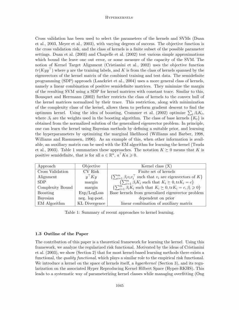
As motivation for the need for methods to learn the kernel, consider Figure 1, which showsthe separating hyperplane, the margin and the training data for a synthetic dataset. Fig-ure 1(a) shows the classification function for a support vector machine using a Gaussianradial basis function (RBF) kernel. The data has been generated using two Gaussian distri-butions with standard deviation 1 in one dimension and 1000 in the other. This differencein scale creates problems for the Gaussian RBF kernel, since it is unable to find a kernelwidth suitable for both directions. Hence, the classification function is dominated by thedimension with large variance. Increasing the value of the regularization parameter, C,and hence decreasing the smoothness of the function results in a hyperplane which is morecomplex, and equally unsatisfactory (Figure 1(b)). The traditional way to handle such datais to normalize each dimension independently.
Instead of normalising the input data, we make the kernel adaptive to allow independentscales for each dimension. This allows the kernel to handle unnormalised data. However, theresulting kernel would be difficult to hand-tune as there may be numerous free variables.In this case, we have a free parameter for each dimension of the input. We ‘learn’ thiskernel by defining a quantity analogous to the risk functional, called the quality functional,which measures the ‘badness’ of the kernel function. The classification function for theabove mentioned data is shown in Figure 1(c). Observe that it captures the scale of eachdimension independently. In general, the solution does not consist of only a single kernelbut a linear combination of them.
(a) Standard Gaussian RBF kernel(C=10)
(b) Standard Gaussian RBF kernel(C=108)
(c) RBF-Hyperkernel with adap-tive widths
Figure 1: For data with highly non-isotropic variance, choosing one scale for all dimensionsleads to unsatisfactory results. Plot of synthetic data, showing the separatinghyperplane and the margins given for a uniformly chosen length scale (left andmiddle) and an automatic width selection (right).
1.2 Related Work
We analyze some recent approaches to learning the kernel by looking at the objective func-tion that is being optimized and the class of kernels being considered. We will see later(Section 2) that this objective function is related to our definition of a quality functional.
1044
Hyperkernels
Cross validation has been used to select the parameters of the kernels and SVMs (Duanet al., 2003, Meyer et al., 2003), with varying degrees of success. The objective function isthe cross validation risk, and the class of kernels is a finite subset of the possible parametersettings. Duan et al. (2003) and Chapelle et al. (2002) test various simple approximationswhich bound the leave one out error, or some measure of the capacity of the SVM. Thenotion of Kernel Target Alignment (Cristianini et al., 2002) uses the objective functiontr(Kyy>) where y are the training labels, and K is from the class of kernels spanned by theeigenvectors of the kernel matrix of the combined training and test data. The semidefiniteprogramming (SDP) approach (Lanckriet et al., 2004) uses a more general class of kernels,namely a linear combination of positive semidefinite matrices. They minimize the marginof the resulting SVM using a SDP for kernel matrices with constant trace. Similar to this,Bousquet and Herrmann (2002) further restricts the class of kernels to the convex hull ofthe kernel matrices normalized by their trace. This restriction, along with minimizationof the complexity class of the kernel, allows them to perform gradient descent to find theoptimum kernel. Using the idea of boosting, Crammer et al. (2002) optimize
∑t βtKt,
where βt are the weights used in the boosting algorithm. The class of base kernels Kt isobtained from the normalized solution of the generalized eigenvector problem. In principle,one can learn the kernel using Bayesian methods by defining a suitable prior, and learningthe hyperparameters by optimizing the marginal likelihood (Williams and Barber, 1998,Williams and Rasmussen, 1996). As an example of this, when other information is avail-able, an auxiliary matrix can be used with the EM algorithm for learning the kernel (Tsudaet al., 2003). Table 1 summarizes these approaches. The notation K 0 means that K ispositive semidefinite, that is for all a ∈ Rn, a>Ka > 0.
Approach Objective Kernel class (K)Cross Validation CV Risk Finite set of kernelsAlignment y>Ky
∑mi=1 βiviv
>i such that vi are eigenvectors of K
SDP margin ∑m
i=1 βiKi such that Ki 0, trKi = cComplexity Bound margin
∑mi=1 βiKi such that Ki 0, trKi = c, βi > 0
Boosting Exp/LogLoss Base kernels from generalized eigenvector problemBayesian neg. log-post. dependent on priorEM Algorithm KL Divergence linear combination of auxiliary matrix
Table 1: Summary of recent approaches to kernel learning.
1.3 Outline of the Paper
The contribution of this paper is a theoretical framework for learning the kernel. Using thisframework, we analyze the regularized risk functional. Motivated by the ideas of Cristianiniet al. (2003), we show (Section 2) that for most kernel-based learning methods there exists afunctional, the quality functional, which plays a similar role to the empirical risk functional.We introduce a kernel on the space of kernels itself, a hyperkernel (Section 3), and its regu-larization on the associated Hyper Reproducing Kernel Hilbert Space (Hyper-RKHS). Thisleads to a systematic way of parameterizing kernel classes while managing overfitting (Ong
1045
Ong, Smola and Williamson
et al., 2002). We give several examples of hyperkernels and recipes to construct others(Section 4). Using this general framework, we consider the specific example of using theregularized risk functional in the rest of the paper. The positive definiteness of the kernelfunction is ensured using the positive definiteness of the kernel matrix (Section 5), and theresulting optimization problem is a semidefinite program. The semidefinite programmingapproach follows that of Lanckriet et al. (2004), with a different constraint due to a differ-ence in regularization (Ong and Smola, 2003). Details of the specific optimization problemsassociated with the C-SVM, ν-SVM, Lagrangian SVM, ν-SVR and one class SVM are de-fined in Section 6. Experimental results for classification, regression and novelty detection(Section 7) are shown. Finally some issues and open problems are discussed (Section 8).
2. Kernel Quality Functionals
We denote by X the space of input data and Y the space of labels (if we have a supervisedlearning problem). Denote by Xtrain := x1, . . . , xm the training data and with Ytrain :=y1, . . . , ym a set of corresponding labels, jointly drawn independently and identically fromsome probability distribution Pr(x, y) on X×Y. We shall, by convenient abuse of notation,generally denote Ytrain by the vector y, when writing equations in matrix notation. Wedenote by K the kernel matrix given by Kij := k(xi, xj) where xi, xj ∈ Xtrain and k is apositive semidefinite kernel function. We also use trK to mean the trace of the matrix and|K| to mean the determinant.
We begin by introducing a new class of functionals Q on data which we will call qualityfunctionals. Note that by quality we actually mean badness or lack of quality, as we wouldlike to minimize this quantity. Their purpose is to indicate, given a kernel k and the trainingdata, how suitable the kernel is for explaining the training data, or in other words, thequality of the kernel for the estimation problem at hand. Such quality functionals may bethe Kernel Target Alignment, the negative log posterior, the minimum of the regularized riskfunctional, or any luckiness function for kernel methods. We will discuss those functionalsafter a formal definition of the quality functional itself.
2.1 Empirical and Expected Quality
Definition 1 (Empirical Quality Functional) Given a kernel k, and data X, Y , we de-fine Qemp(k, X, Y ) to be an empirical quality functional if it depends on k only via k(xi, xj)where xi, xj ∈ X for 1 6 i, j 6 m.
By this definition, Qemp is a function which tells us how well matched k is to a specificdataset X, Y . Typically such a quantity is used to adapt k in such a manner that Qemp isoptimal (for example, optimal Kernel Target Alignment, greatest luckiness, smallest nega-tive log-posterior), based on this one single dataset X, Y . Provided a sufficiently rich classof kernels K it is in general possible to find a kernel k∗ ∈ K that attains the minimumof any such Qemp regardless of the data. However, it is very unlikely that Qemp(k∗, X, Y )would be similarly small for other X, Y , for such a k∗. To measure the overall quality of kwe therefore introduce the following definition:
1046
Hyperkernels
Definition 2 (Expected Quality Functional) Denote by Qemp(k, X, Y ) an empiricalquality functional, then
Q(k) := EX,Y [Qemp(k, X, Y )]
is defined to be the expected quality functional. Here the expectation is taken over X, Y ,where all xi, yi are drawn from Pr(x, y).
Observe the similarity between the empirical quality functional, Qemp(k, X, Y ), and theempirical risk of an estimator, Remp(f,X, Y ) = 1
m
∑mi=1 l(xi, yi, f(xi)) (where l is a suitable
loss function); in both cases we compute the value of a functional which depends on somesample X, Y drawn from Pr(x, y) and a function and in both cases we have
Q(k) = EX,Y [Qemp(k, X, Y )] and R(f) = EX,Y [Remp(f,X, Y )] .
Here R(f) denotes the expected risk. However, while in the case of the empirical risk we caninterpret Remp as the empirical estimate of the expected loss R(f) = Ex,y[l(x, y, f(x))], dueto the general form of Qemp, no such analogy is available for quality functionals. Finding ageneral-purpose bound of the expected error in terms of Q(k) is difficult, since the definitionof Q depends heavily on the algorithm under consideration. Nonetheless, it provides ageneral framework within which such bounds can be derived.
To obtain a generalization error bound, it is sufficient that Qemp is concentrated aroundits expected value. Furthermore, one would require the deviation of the empirical risk to beupper bounded by Qemp and possibly other terms. In other words, we assume a) we havegiven a concentration inequality on quality functionals, such as
Pr |Qemp(k, X, Y )−Q(k)| > εQ < δQ,
and b) we have a bound on the deviation of the empirical risk in terms of the qualityfunctional
Pr |Remp(f,X, Y )−R(f)| > εR < δ(Qemp).
Then we can chain both inequalities together to obtain the following bound
Pr |Remp(f,X, Y )−R(f)| > εR < δQ + δ(Q + εQ).
This means that the bound now becomes independent of the particular value of the qualityfunctional obtained on the data, rather than the expected value of the quality functional.Bounds of this type have been derived for Kernel Target Alignment (Cristianini et al.,2003, Theorem 9) and the Algorithmic Luckiness framework (Herbrich and Williamson,2002, Theorem 17).
2.2 Examples of Qemp
Before we continue with the derivations of a regularized quality functional and introduce acorresponding Reproducing Kernel Hilbert Space, we give some examples of quality func-tionals and present their exact minimizers, whenever possible. This demonstrates that givena rich enough feature space, we can arbitrarily minimize the empirical quality functionalQemp. The difference here from traditional kernel methods is the fact that we allow the
1047
Ong, Smola and Williamson
kernel to change. This extra degree of freedom allows us to overfit the training data. Inmany of the examples below, we show that given a feature mapping which can model thelabels of the training data precisely, overfitting occurs. That is, if we use the training labelsas the kernel matrix, we arbitrarily minimize the quality functional. The reader who isconvinced that one can arbitrarily minimize Qemp, by optimizing over a suitably large classof kernels, may skip the following examples.
Example 1 (Regularized Risk Functional) These are commonly used in SVMs andrelated kernel methods (see Wahba (1990), Vapnik (1995), Scholkopf and Smola (2002)).They take on the general form
Rreg(f,Xtrain, Ytrain) :=1m
m∑i=1
l(xi, yi, f(xi)) +λ
2‖f‖2
H (1)
where ‖f‖2H is the RKHS norm of f and l is a loss function such that for f(xi) = yi,
l(xi, yi, yi) = 0. By virtue of the representer theorem (see Section 3) we know that theminimizer of (1) can be written as a kernel expansion. This leads to the following definitionof a quality functional, for a particular loss functional l:
Qregriskemp (k, Xtrain, Ytrain) := min
α∈Rm
[1m
m∑i=1
l(xi, yi, [Kα]i) +λ
2α>Kα
]. (2)
The minimizer of (2) is somewhat difficult to find, since we have to carry out a doubleminimization over K and α. However, we know that Qregrisk
emp is bounded from below by 0.Hence, it is sufficient if we can find a (possibly) suboptimal pair (α, k) for which Qregrisk
emp ≤ εfor any ε > 0:
• Note that for K = βyy> and α = 1β‖y‖2 y we have Kα = y and α>Kα = β−1. This
leads to l(xi, yi, f(xi)) = 0 and therefore Qregriskemp (k, Xtrain, Ytrain) = λ
2β . For sufficiently
large β we can make Qregriskemp (k, Xtrain, Ytrain) arbitrarily close to 0.
• Even if we disallow setting K arbitrarily close to zero by setting trK = 1, finding theminimum of (2) can be achieved as follows: let K = 1
‖z‖2 zz>, where z ∈ Rm, andα = z. Then Kα = z and we obtain
1m
m∑i=1
l(xi, yi, [Kα]i) +λ
2α>Kα =
m∑i=1
l(xi, yi, zi) +λ
2‖z‖2
2. (3)
Choosing each zi = argminζ l(xi, yi, ζ(xi)) + λ2 ζ2, where ζ are the possible hypothe-
sis functions obtained from the training data, yields the minimum with respect to z.Since (3) tends to zero and the regularized risk is lower bounded by zero, we can stillarbitrarily minimize Qregrisk
emp . This is not surprising since the set of allowable K ishuge.
Example 2 (Cross Validation) Cross validation is a widely used method for estimat-ing the generalization error of a particular learning algorithm. Specifically, the leave-one-out cross validation is an almost unbiased estimate of the generalization error (Luntz and
1048
Hyperkernels
Brailovsky, 1969). The quality functional for classification using kernel methods is givenby:
Qlooemp(k, Xtrain, Ytrain) := min
α∈Rm
[1m
m∑i=1
−yi sign([Kαi]i)
],
which is optimized in Duan et al. (2003), Meyer et al. (2003).Choosing K = yy> and αi = 1
‖yi‖2 yi, where αi and yi are the vectors α and y with the ithelement set to zero, we have Kαi = yi. Hence we can match the training data perfectly. Fora validation set of larger size, i.e. k-fold cross validation, the same result can be achievedby defining a corresponding α.
Example 3 (Kernel Target Alignment) This quality functional was introduced by Cris-tianini et al. (2002) to assess the alignment of a kernel with training labels. It is definedby
Qalignmentemp (k, Xtrain, Ytrain) := 1− tr(Kyy>)
‖y‖22‖K‖F
. (4)
Here ‖y‖2 denotes the `2 norm of the vector of observations and ‖K‖F is the Frobeniusnorm, i.e., ‖K‖2
F := tr(KK>) =∑
i,j(Kij)2. This quality functional was optimized inLanckriet et al. (2004). By decomposing K into its eigensystem one can see that (4) isminimized, if K = yy>, in which case
Qalignmentemp (k∗, Xtrain, Ytrain) = 1− tr(y>yy>y)
‖y‖22‖yy>‖F
= 1− ‖y‖42
‖y‖22‖y‖2
2
= 0.
We cannot expect that Qalignmentemp (k∗, X, Y ) = 0 for data other than that chosen to determine
k∗, in other words, a restriction of the class of kernels is required. This was also observedin Cristianini et al. (2003).
The above examples illustrate how existing methods for assessing the quality of a kernelfit within the quality functional framework. We also saw that given a rich enough class ofkernels K, optimization of Qemp over K would result in a kernel that would be useless forprediction purposes, in the sense that they can be made to look arbitrarily good in termsof Qemp but with the result that the generalization performance will be poor. This is yetanother example of the danger of optimizing too much and overfitting – there is (still) nofree lunch.
3. Hyper Reproducing Kernel Hilbert Spaces
We now propose a conceptually simple method to optimize quality functionals over classesof kernels by introducing a Reproducing Kernel Hilbert Space on the kernel k itself, so tosay, a Hyper-RKHS. We first review the definition of a RKHS (Aronszajn, 1950).
Definition 3 (Reproducing Kernel Hilbert Space) Let X be a nonempty set (the in-dex set) and denote by H a Hilbert space of functions f : X → R. H is called a reproducingkernel Hilbert space endowed with the dot product 〈·, ·〉 (and the norm ‖f‖ :=
√〈f, f〉) if
there exists a function k : X× X → R with the following properties.
1049
Ong, Smola and Williamson
1. k has the reproducing property
〈f, k(x, ·)〉 = f(x) for all f ∈ H, x ∈ X;
in particular, 〈k(x, ·), k(x′, ·)〉 = k(x, x′) for all x, x′ ∈ X.
2. k spans H, i.e. H = spank(x, ·)|x ∈ X where X is the completion of the set X.
In the rest of the paper, we use the notation k to represent the kernel function and H torepresent the RKHS. In essence, H is a Hilbert space of functions, which has the specialproperty of being generated by the kernel function k.
The advantage of optimization in an RKHS is that under certain conditions the optimalsolutions can be found as the linear combination of a finite number of basis functions,regardless of the dimensionality of the space H the optimization is carried out in. Thetheorem below formalizes this notion (see Kimeldorf and Wahba (1971), Cox and O’Sullivan(1990)).
Theorem 4 (Representer Theorem) Denote by Ω : [0,∞) → R a strictly monotonicincreasing function, by X a set, and by l : (X×R2)m → R∪∞ an arbitrary loss function.Then each minimizer f ∈ H of the general regularized risk
l ((x1, y1, f(x1)) , . . . , (xm, ym, f(xm))) + Ω (‖f‖H)
admits a representation of the form
f(x) =m∑
i=1
αik(xi, x), (5)
where αi ∈ R for all 1 6 i 6 m.
3.1 Regularized Quality Functional
To learn the kernel, we need to define a function space of kernels, a method to regularizethem and a practical optimization procedure. We will address each of these issues in thefollowing. We define a RKHS on kernels k : X × X → R, simply by introducing thecompounded index set, X := X× X and by treating k as a function k : X → R:
Definition 5 (Hyper Reproducing Kernel Hilbert Space) Let X be a nonempty set.and denote by X := X × X the compounded index set. The Hilbert space H of functionsk : X → R, endowed with a dot product 〈·, ·〉 (and the norm ‖k‖ =
√〈k, k〉) is called a
Hyper Reproducing Kernel Hilbert Space if there exists a hyperkernel k : X × X → R withthe following properties:
1. k has the reproducing property 〈k, k(x, ·)〉 = k(x) for all k ∈ H; in particular, 〈k(x, ·), k(x′, ·)〉 =k(x, x′).
2. k spans H, i.e. H = spank(x, ·)|x ∈ X.
3. k(x, y, s, t) = k(y, x, s, t) for all x, y, s, t ∈ X.
1050
Hyperkernels
This is a RKHS with the additional requirement of symmetry in its first two arguments(in fact, we can have a recursive definition of an RKHS of an RKHS ad infinitum, withsuitable restrictions on the elements). We define the corresponding notations for elements,kernels, and RKHS by underlining it. What distinguishes H from a normal RKHS is theparticular form of its index set (X = X2) and the additional condition on k to be symmetricin its first two arguments, and therefore in its second two arguments as well.
This approach of defining a RKHS on the space of symmetric functions of two variablesleads us to a natural regularization method. By analogy with the definition of the regularizedrisk functional (1), we proceed to define the regularized quality functional.
Definition 6 (Regularized Quality Functional) Let X, Y be the combined training andtest set of examples and labels respectively. For a positive semidefinite kernel matrix K onX, the regularized quality functional is defined as
Qreg(k, X, Y ) := Qemp(k, X, Y ) +λQ
2‖k‖2
H, (6)
where λQ > 0 is a regularization constant and ‖k‖2H denotes the RKHS norm in H.
Note that although we have possibly non positive kernels in H, we define the regularizedquality functional only on positive semidefinite kernel matrices. This is a slightly weakercondition than requiring a positive semidefinite kernel k, since we only require positivityon the data. Since Qemp depends on k only via the data, this is sufficient for the abovedefinition. Minimization of Qreg is less prone to overfitting than minimizing Qemp, sincethe regularization term λQ
2 ‖k‖2H effectively controls the complexity of the class of kernels
under consideration. Bousquet and Herrmann (2002) provide a generalization error boundby estimating the Rademacher complexity of the kernel classes in the transduction setting.Regularizers other than ‖k‖2
H are possible, such as `p penalties. In this paper, we restrictourselves to the `2 norm (6). The advantage of (6) is that its minimizer satisfies therepresenter theorem.
Lemma 7 (Representer Theorem for Hyper-RKHS) Let X be a set, Qemp an arbi-trary empirical quality functional, and X, Y the combined training and test set, then eachminimizer k ∈ H of the regularized quality functional Qreg(k, X, Y ) admits a representationof the form
k(x, x′) =m∑i,j
βijk((xi, xj), (x, x′)) for all x, x′ ∈ X, (7)
where βij ∈ R, for each 1 6 i, j 6 m.
Proof All we need to do is rewrite (6) so that it satisfies the conditions of Theorem 4. Letxij := (xi, xj). Then Qemp(k, X, Y ) has the properties of a loss function, as it only dependson k via its values at xij . Note too that the kernel matrix K also only depends on k via
its values at xij . Furthermore, λQ
2 ‖k‖2H is an RKHS regularizer, so the representer theorem
applies and (7) follows.
Lemma 7 implies that the solution of the regularized quality functional is a linear combina-tion of hyperkernels on the input data. This shows that even though the optimization takes
1051
Ong, Smola and Williamson
place over an entire Hilbert space of kernels, one can find the optimal solution by choosingamong a finite number.
Note that the minimizer (7) is not necessarily positive semidefinite. In practice, this isnot what we want, since we require a positive semidefinite kernel but we do not have anyguarantees for examples in the test set. Therefore we need to impose additional constraintsof the type K 0 or k is a Mercer Kernel. While the latter is almost impossible to enforcedirectly, the former could be verified directly, hence imposing a constraint only on the valuesof the kernel matrix k(xi, xj) rather than on the kernel function k itself. This means thatthe conditions of the Representer Theorem apply and (7) applies (with suitable constraintson the coefficients βij).
Another option is to be somewhat more restrictive and require that all expansion coeffi-cients βi,j > 0 and all the functions be positive semidefinite kernels. This latter requirementcan be formally stated as follows: For any fixed x ∈ X the hyperkernel k is a kernel in itssecond argument; that is for any fixed x ∈ X, the function k(x, x′) := k(x, (x, x′)), withx, x′ ∈ X, is a positive semidefinite kernel.
Proposition 8 Given a hyperkernel, k with elements such that for any fixed x ∈ X, thefunction k(xp, xq) := k(x, (xp, xq)), with xp, xq ∈ X, is a positive semidefinite kernel, andβij > 0 for all i, j = 1, . . . ,m, then the kernel
k(xp, xq) :=m∑
i,j=1
βijk(xi, xj , xp, xq)
is positive semidefinite.
Proof The result is obtained by observing that positive combinations of positive semidef-inite kernels are positive semidefinite.
While this may prevent us from obtaining the minimizer of the objective function, ityields a much more amenable optimization problem in practice, in particular if the resultingcone spans a large enough space (as happens with increasing m). In the subsequent deriva-tions of optimization problems, we choose this restriction as it provides a more tractableproblem in practice. In Section 4, we give examples and recipes for constructing hyperker-nels. Before that, we relate our framework defined above to Bayesian inference.
3.2 A Bayesian Perspective
A generative Bayesian approach to inference encodes all knowledge we might have aboutthe problem setting into a prior distribution. Hence, the choice of the prior distributiondetermines the behaviour of the inference, as once we have the data, we condition onthe prior distribution we have chosen to obtain the posterior, and then marginalize toobtain the label that we are interested in. One popular choice of prior is the normaldistribution, resulting in a Gaussian process (GP). All prior knowledge we have about theproblem is then encoded in the covariance of the GP. There exists a GP analog to theSupport Vector Machine (for example Opper and Winther (2000), Seeger (1999)), which
1052
Hyperkernels
is essentially obtained (ignoring normalizing terms) by exponentiating the regularized riskfunctional used in SVMs.
In this section, we derive the prior and hyperprior implied by our framework of hyperk-ernels. This is obtained by exponentiating Qreg, again ignoring normalization terms. Giventhe regularized quality functional (Equation 6), with the Qemp set to the SVM with squaredloss, we obtain the following equation.
Qreg(k, X, Y ) :=1m
m∑i=1
(yi − f(xi))2 +λ
2‖f‖2
H +λQ
2‖k‖2
H.
Exponentiating the negative of the above equation gives,
exp(−Qreg(k, X, Y )) =
exp
(− 1
m
m∑i=1
(yi − f(xi))2)
exp(−λ
2‖f‖2
H
)exp
(−
λQ
2‖k‖2
H
).
(8)
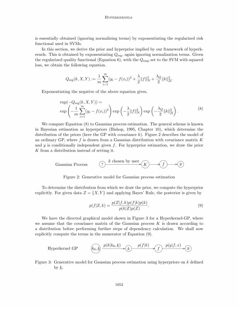
We compare Equation (8) to Gaussian process estimation. The general scheme is knownin Bayesian estimation as hyperpriors (Bishop, 1995, Chapter 10), which determine thedistribution of the priors (here the GP with covariance k). Figure 2 describes the model ofan ordinary GP, where f is drawn from a Gaussian distribution with covariance matrix Kand y is conditionally independent given f . For hyperprior estimation, we draw the priorK from a distribution instead of setting it.
Gaussian Process ?>=<89:;?k chosen by user // GFED@ABCK //GFED@ABCf // ?>=<89:;y
Figure 2: Generative model for Gaussian process estimation
To determine the distribution from which we draw the prior, we compute the hyperpriorexplicitly. For given data Z = X, Y and applying Bayes’ Rule, the posterior is given by
p(f |Z, k) =p(Z|f, k)p(f |k)p(k)
p(k|Z)p(Z). (9)
We have the directed graphical model shown in Figure 3 for a Hyperkernel-GP, wherewe assume that the covariance matrix of the Gaussian process K is drawn according toa distribution before performing further steps of dependency calculation. We shall nowexplicitly compute the terms in the numerator of Equation (9).
Hyperkernel GP ONMLHIJKk0, kp(k|k0, k)
// ?>=<89:;kp(f |k)
//GFED@ABCfp(y|f, x)
// ?>=<89:;y
Figure 3: Generative model for Gaussian process estimation using hyperpriors on k definedby k.
1053
Ong, Smola and Williamson
In the following derivations, we assume that we are dealing with finite dimensionalobjects, to simplify the calculations of the normalizing constants in the expressions for thedistributions. Given that we have additive Gaussian noise, that is ε ∼ N(0, 1
γεI), then,
p(y|f, x) ∝ exp(−γε
2(y − f(x))2
).
Therefore, for the whole dataset (assumed to be i.i.d.),
p(Y |f,X) =m∏
i=1
p(yi|f, xi) =(
2π
γε
)−m2
exp
(−γε
2
m∑i=1
(yi − f(xi))2)
.
We assume a Gaussian prior on the function f , with covariance function k. The positivesemidefinite function, k, defines an inner product 〈·, ·〉Hk
in the RKHS denoted by Hk.Then,
p(f |k) =(
2π
γf
)−F2
exp(−
γf
2〈f, f〉Hk
)where F is the dimension of f and γf is a constant.
We assume a Wishart distribution (Lauritzen, 1996, Appendix C), with p degrees offreedom and covariance k0, for the prior distribution of the covariance function k, that isk ∼ Wm(p, k0). This is a hyperprior used in the Gaussian process literature.
p(k|k0) =|k|
p−(m+1)2 exp
(−1
2tr(kk0))
Γm(p)|k|p2
where Γm(p) denotes the Gamma distribution, Γm(p) = 2pm2 π
m(m−1)4
∏mi=1 Γ
(p−i+1
2
). For
more details of the Wishart distribution, the reader is referred to Lauritzen (1996).Observe that tr(kk0) is an inner product between two matrices. We can define a general
inner product between two matrices, as the inner product defined in the RKHS denoted byH.
p(k|k0, k) =|k|
p−(m+1)2 exp
(−1
2〈k, k0〉H)
Γm(p)|k|p2
We can interpret the above equation as measuring the similarity between the covariancematrix that we obtain from data and the expected covariance matrix (given by the user).This similarity is measured by a dot product defined by k. Substituting the expressionsfor p(Y |X, f), p(f |k) and p(k|k0, k) into the posterior (Equation 9), we get Equation (10)which is of the same form as the exponentiated negative quality (Equation 8).
exp
(−γε
2
m∑i=1
(yi − f(xi))2)
exp(−
γf
2〈f, f〉Hk
)exp
(−1
2〈k, k0〉H
). (10)
In a nutshell, we assume that the covariance function of the GP k, is distributed accord-ing to a Wishart distribution. In other words, we have two nested processes, a Gaussian and
1054
Hyperkernels
a Wishart process, to model the data generation scheme. Hence we are studying a mixtureof Gaussian processes. Note that the maximum likelihood (ML-II) estimator (MacKay,1994, Williams and Barber, 1998, Williams and Rasmussen, 1996) in Bayesian estimationleads to the same optimization problems as those arising from minimizing the regularizedquality functional.
4. Hyperkernels
Having introduced the theoretical basis of the Hyper-RKHS, it is natural to ask whetherhyperkernels, k, exist which satisfy the conditions of Definition 5. We address this questionby giving a set of general recipes for building such kernels.
4.1 Power Series Construction
Suppose k is a kernel such that k(x, x′) ≥ 0 for all x, x′ ∈ X, and suppose g : R → R isa function with positive Taylor expansion coefficients, that is g(ξ) =
∑∞i=0 ciξ
i for basisfunctions ξ, ci > 0 for all i = 0, . . . ,∞, and convergence radius R. Then for pointwisepositive k(x, x′) ≤
√R,
k(x, x′) := g(k(x)k(x′)) =∞∑i=0
ci(k(x)k(x′))i (11)
is a hyperkernel. For k to be a hyperkernel, we need to check that first, k is a kernel, andsecond, for any fixed pair of elements of the input data, x, the function k(x, (x, x′)) is akernel, and third that is satisfies the symmetry condition. Here, the symmetry conditionfollows from the symmetry of k. To see this, observe that for any fixed x, k(x, (x, x′))is a sum of kernel functions, hence it is a kernel itself (since kp(x, x′) is a kernel if kis, for p ∈ N). To show that k is a kernel, note that k(x, x′) = 〈Φ(x),Φ(x′)〉, whereΦ(x) := (
√c0,
√c1k
1(x),√
c2k2(x), . . .). Note that we require pointwise positivity, so that
the coefficients of the sum in Equation (11) are always positive. The Gaussian RBF kernelsatisfies this condition, but polynomial kernels of odd degree are not always pointwisepositive. In the following example, we use the Gaussian kernel to construct a hyperkernel.
Example 4 (Harmonic Hyperkernel) Suppose k is a kernel with range [0, 1], (RBFkernels satisfy this property), and set ci := (1 − λh)λi
h, i ∈ N, for some 0 < λh < 1. Thenwe have
k(x, x′) = (1− λh)∞∑i=0
(λhk(x)k(x′)
)i =1− λh
1− λhk(x)k(x′). (12)
For k(x, x′) = exp(−σ2‖x− x′‖2) this construction leads to
k((x, x′), (x′′, x′′′)) =1− λh
1− λh exp (−σ2(‖x− x′‖2 + ‖x′′ − x′′′‖2)). (13)
As one can see, for λh → 1, k converges to δx,x′, and thus ‖k‖2H converges to the Frobenius
norm of k on X ×X.
1055
Ong, Smola and Williamson
g(ξ) Power series expansion Radius of Convergenceexp ξ 1 + 1
1!ξ + 12!ξ
2 + 13!ξ
3 + . . . + 1n!ξ
n + . . . ∞sinh ξ 1
1!ξ + 13!ξ
3 + 15!ξ
5 + . . . + 1(2n+1)!ξ
(2n+1) + . . . ∞cosh ξ 1 + 1
2!ξ2 + 1
4!ξ4 + . . . + 1
(2n)!ξ(2n) + . . . ∞
arctanhξ ξ1 + ξ3
3 + ξ5
5 + . . . + ξ2n+1
2n+1 + . . . 1
− ln(1− ξ) ξ1 + ξ2
2 + ξ3
3 + . . . + ξn
n + . . . 1
Table 2: Hyperkernels by Power Series Construction.
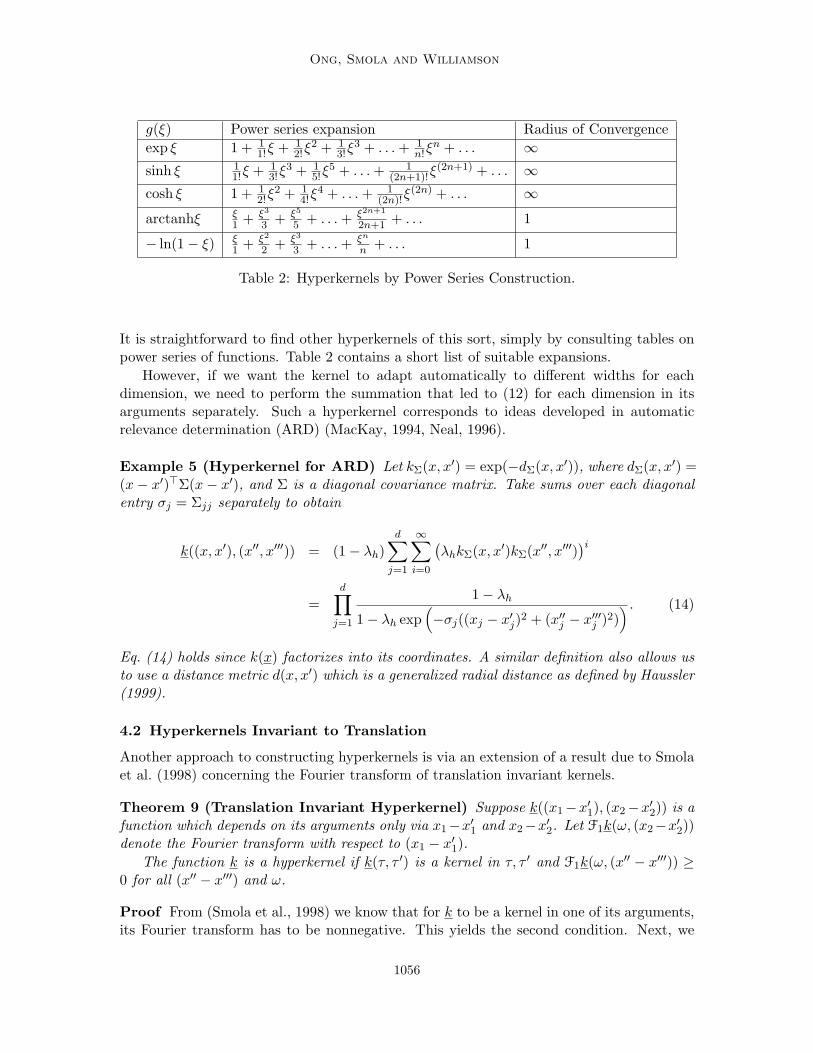
It is straightforward to find other hyperkernels of this sort, simply by consulting tables onpower series of functions. Table 2 contains a short list of suitable expansions.
However, if we want the kernel to adapt automatically to different widths for eachdimension, we need to perform the summation that led to (12) for each dimension in itsarguments separately. Such a hyperkernel corresponds to ideas developed in automaticrelevance determination (ARD) (MacKay, 1994, Neal, 1996).
Example 5 (Hyperkernel for ARD) Let kΣ(x, x′) = exp(−dΣ(x, x′)), where dΣ(x, x′) =(x− x′)>Σ(x− x′), and Σ is a diagonal covariance matrix. Take sums over each diagonalentry σj = Σjj separately to obtain
k((x, x′), (x′′, x′′′)) = (1− λh)d∑
j=1
∞∑i=0
(λhkΣ(x, x′)kΣ(x′′, x′′′)
)i=
d∏j=1
1− λh
1− λh exp(−σj((xj − x′j)2 + (x′′j − x′′′j )2)
) . (14)
Eq. (14) holds since k(x) factorizes into its coordinates. A similar definition also allows usto use a distance metric d(x, x′) which is a generalized radial distance as defined by Haussler(1999).
4.2 Hyperkernels Invariant to Translation
Another approach to constructing hyperkernels is via an extension of a result due to Smolaet al. (1998) concerning the Fourier transform of translation invariant kernels.
Theorem 9 (Translation Invariant Hyperkernel) Suppose k((x1−x′1), (x2−x′2)) is afunction which depends on its arguments only via x1−x′1 and x2−x′2. Let F1k(ω, (x2−x′2))denote the Fourier transform with respect to (x1 − x′1).
The function k is a hyperkernel if k(τ, τ ′) is a kernel in τ, τ ′ and F1k(ω, (x′′ − x′′′)) ≥0 for all (x′′ − x′′′) and ω.
Proof From (Smola et al., 1998) we know that for k to be a kernel in one of its arguments,its Fourier transform has to be nonnegative. This yields the second condition. Next, we
1056
Hyperkernels
need to show that k is a kernel in its own right. Mercer’s condition requires that for arbitraryf the following is positive:∫
f(x1, x′1)f(x2, x
′2)k((x1 − x′1), (x2 − x′2))dx1dx′1dx2dx′2
=∫
f(τ1 + x′1, x′1)f(τ2 + x′2, x
′2)dx1,2k(τ1, τ2)dτ1dτ2
=∫
g(τ1)g(τ2)k(τ1, τ2)dτ1dτ2,
where τ1 = x1 − x′1 and τ2 = x2 − x′2. Here g is obtained by integration over x1 and x2
respectively. The latter is exactly Mercer’s condition on k, when viewed as a function oftwo variables only.
This means that we can check whether a radial basis function (for example Gaussian RBF,exponential RBF, damped harmonic oscillator, generalized Bn spline), can be used to con-struct a hyperkernel by checking whether its Fourier transform is positive.
4.3 Explicit Expansion
If we have a finite set of kernels that we want to choose from, we can generate a hyperkernelwhich is a finite sum of possible kernel functions. This setting is similar to that of Lanckrietet al. (2004).
Suppose ki(x, x′) is a kernel for each i = 1, . . . , n (for example the RBF kernel or thepolynomial kernel), then
k(x, x′) :=n∑
i=1
ciki(x)ki(x′), ki(x) > 0,∀x (15)
is a hyperkernel, as can be seen by an argument similar to that of section 4.1. k is a kernelsince k(x, x′) = 〈Φ(x),Φ(x′)〉, where Φ(x) := (
√c1k1(x),
√c2k2(x), . . . ,
√cnkn(x)).
Example 6 (Polynomial and RBF combination) Let k1(x, x′) = (〈x, x′〉 + b)2p forsome choice of b ∈ R+ and p ∈ N, and k2(x, x′) = exp(−σ2‖x− x′‖2). Then,
k((x1, x′1), (x2, x
′2)) = c1(〈x1, x
′1〉+ b)2p(〈x2, x
′2〉+ b)2p
+c2 exp(−σ2‖x1 − x′1‖2) exp(−σ2‖x2 − x′2‖2)(16)
is a hyperkernel.
5. Optimization Problems for Regularized Risk based Quality Functionals
We will now consider the optimization of the quality functionals utilizing hyperkernels. Wechoose the regularized risk functional as the empirical quality functional; that is we setQemp(k, X, Y ) := Rreg(f,X, Y ). It is possible to utilize other quality functionals, such asthe Kernel Target Alignment (Example 12). We focus our attention on the regularized riskfunctional, which is commonly used in SVMs. Furthermore, we will only consider positivesemidefinite kernels. For a particular loss function l(xi, yi, f(xi)), we obtain the regularizedquality functional.
mink∈H
minf∈Hk
1m
m∑i=1
l(xi, yi, f(xi)) +λ
2‖f‖2
Hk+
λQ
2‖k‖2
H. (17)
1057
Ong, Smola and Williamson
By the representer theorem (Theorem 4 and Corollary 7) we can write the regularizersas quadratic terms. Using the soft margin loss, we obtain
minβ
minα
1m
m∑i=1
max(0, 1− yif(xi)) +λ
2α>Kα +
λQ
2β>Kβ subject to β > 0 (18)
where α ∈ Rm are the coefficients of the kernel expansion (5), and β ∈ Rm2are the
coefficients of the hyperkernel expansion (7).For fixed k, the problem can be formulated as a constrained minimization problem in f ,
and subsequently expressed in terms of the Lagrange multipliers α. However, this minimumdepends on k, and for efficient minimization we would like to compute the derivatives withrespect to k. The following lemma tells us how (it is an extension of a result in Chapelleet al. (2002)):
Lemma 10 Let x ∈ Rm and denote by f(x, θ), ci : Rm → R convex functions, where f isparameterized by θ. Let R(θ) be the minimum of the following optimization problem (anddenote by x(θ) its minimizer):
minimizex∈Rm
f(x, θ) subject to ci(x) ≤ 0 for all 1 ≤ i ≤ n.
Then ∂jθR(θ) = Dj
2f(x(θ), θ), where j ∈ N and D2 denotes the derivative with respect to thesecond argument of f .
Proof At optimality we have a saddlepoint in the Lagrangian
∂xL(x, α) = ∂xf(x, θ) +n∑
i=1
αi∂xci(x) = 0. (19)
Furthermore, for all θ the Kuhn-Tucker conditions have to hold, and in particular also∑ni=1 αi∂θci(x(θ)) = 0, since for all αi > 0 the condition ci(x) = 0 and therefore also
∂θci(x(θ)) = 0 has to be satisfied. Taking higher order derivatives with respect to θ yields
0 = ∂jθ
[n∑
i=1
αi∂xci(x(θ))∂x
∂θ
]= ∂j
θ
[−∂xf(x, θ)
∂x
∂θ
]. (20)
Here the last equality follows from (19). Next we use
∂j+1θ f(x, θ) = ∂j
θ
[D2f(x, θ) + ∂xf(x, θ)
∂x
∂θ
]= ∂j
θD2f(x, θ).
Repeated application then proves the claim.
Instead of directly minimizing Equation (18), we derive the dual formulation. Usingthe approach in Lanckriet et al. (2004), the corresponding optimization problems can beexpressed as a SDP. In general, solving a SDP would be take longer than solving a quadratic
1058
Hyperkernels
program (a traditional SVM is a quadratic program). This reflects the added cost incurredfor optimizing over a class of kernels.
Semidefinite programming (Vandenberghe and Boyd, 1996) is the optimization of alinear objective function subject to constraints which are linear matrix inequalities andaffine equalities.
Definition 11 (Semidefinite Program) A semidefinite program (SDP) is a problem ofthe form:
minx
c>x
subject to F0 +q∑
i=1
xiFi 0 and Ax = b
where x ∈ Rp are the decision variables, A ∈ Rp×q, b ∈ Rp, c ∈ Rq, and Fi ∈ Rr×r aregiven.
In general, linear constraints Ax + a > 0 can be expressed as a semidefinite constraintdiag(Ax + a) 0, and a convex quadratic constraint (Ax + b)>(Ax + b)− c>x− d 6 0 canbe written as [
I Ax + b(Ax + b)> c>x + d
] 0.
When t ∈ R, we can write the quadratic constraint a>Aa 6 t as ‖A12 a‖ 6 t. In practice,
linear and quadratic constraints are simpler and faster to implement in a convex solver.We derive the corresponding SDP for Equation (17). The following proposition allows us
to derive a SDP from a class of general convex programs. It follows the approach in Lanckrietet al. (2004), with some care taken with Schur complements of positive semidefinite matrices(Albert, 1969), and its proof is omitted for brevity.
Proposition 12 (Quadratic Minimax) Let m,n,M ∈ N, H : Rn → Rm×m, c : Rn →Rm, be linear maps. Let A ∈ RM×m and a ∈ RM . Also, let d : Rn → R and G(ξ) be afunction and the further constraints on ξ. Then the optimization problem
minimizeξ∈Rn
maximizex∈Rm
−12x>H(ξ)x− c(ξ)>x + d(ξ)
subject to H(ξ) 0Ax + a > 0G(ξ) 0
(21)
can be rewritten as
minimizet,ξ,γ
12 t + a>γ + d(ξ)
subject to
diag(γ) 0 0 0
0 G(ξ) 0 00 0 H(ξ) (A>γ − c(ξ))0 0 (A>γ − c(ξ))> t
0(22)
in the sense that the ξ which solves (22) also solves (21).
1059
Ong, Smola and Williamson
Specifically, when we have the regularized quality functional, d(ξ) is quadratic, and hencewe obtain an optimization problem which has a mix of linear, quadratic and semidefiniteconstraints.
Corollary 13 Let H, c, A and a be as in Proposition 12, and Σ 0. Then the solution ξ∗
to the optimization problem
minimizeξ
maximizex
−12x>H(ξ)x− c(ξ)>x + 1
2ξ>Σξ
subject to H(ξ) 0Ax + a > 0ξ > 0
(23)
can be found by solving the semidefinite programming problem
minimizet,t′,ξ,γ
12 t + 1
2 t′ + a>γ
subject to γ > 0ξ > 0‖Σ
12 ξ‖2 6 t′[
H(ξ) (A>γ − c(ξ))(A>γ − c(ξ))> t
] 0
(24)
Proof By applying proposition 12, and introducing an auxiliary variable t′ which upperbounds the quadratic term of ξ, the claim is proved.
Comparing the objective function in (21) with (18), we observe that H(ξ) and c(ξ) arelinear in ξ. Let ξ′ = εξ. As we vary ε the constraints are still satisfied, but the objectivefunction scales with ε. Since ξ is the coeffient in the hyperkernel expansion, this impliesthat we have a set of possible kernels which are just scalar multiples of each other. To avoidthis, we add an additional constraint on ξ which is 1>ξ = c, where c is a constant. Thisbreaks the scaling freedom of the kernel matrix. As a side-effect, the numerical stability ofthe SDP problems improves considerably. We chose a linear constraint so that it does notadd too much overhead to the optimization problem We make one additional simplificationof the optimization problem, which is to replace the upper bound of the squared norm(‖Σ
12 ξ‖2 6 t′) with and upper bound on the norm (‖Σ
12 ξ‖ 6 t′).
In our setting, the regularizer for controlling the complexity of the kernel is taken tobe the squared norm of the kernel in the Hyper-RKHS. By looking at the constraintsof Equation (24), this is expressed as a bound on the norm (‖Σ
12 ξ‖ 6 t′). Comparing
this result to the SDP obtained in Lanckriet et al. (2004, Theorem 16), we see that thecorresponding regularizer in their setting is tr(K) = c, where c is a constant. Hence the maindifference between the two SDPs is the choice of the regularizer for the kernel. However, themotivations of the two methods are different. This paper sets out an induction frameworkfor learning the kernel, and for a particular choice of Qemp, namely the regularized riskfunctional, we obtain an SDP which has similarities to the approach of Lanckriet et al.(2004). On the other hand, they start out with a transduction problem and derive theoptimization problem directly. It is unclear at this point which is the better approach.
1060
Hyperkernels
From the general framework above (Corollary 13, we derive several examples of ma-chine learning problems, specifically binary classification, regression, and single class (alsoknown as novelty detection) problems. The following examples illustrate our method forsimultaneously optimizing over the class of kernels induced by the hyperkernel, as well asthe hypothesis class of the machine learning problem. We consider machine learning prob-lems based on kernel methods which are derived from (17). The derivation is essentially byapplication of Corollary 13 with the two additional conditions above.
6. Examples of Hyperkernel Optimization Problems
In this section, we define the following notation. For p, q, r ∈ Rn, n ∈ N let r = p q bedefined as element by element multiplication, ri = pi× qi (the Hadamard product, or the .∗operation in Matlab). The pseudo-inverse (also known as the Moore-Penrose inverse) of amatrix K is denoted K†. Let ~K be the m2 by 1 vector formed by concatenating the columnsof an m by m matrix. We define the hyperkernel Gram matrix K by putting together m2
of these vectors, that is we set K = [ ~Kpq]mp,q=1. Other notations include: the kernel matrixK = reshape(Kβ) (reshaping a m2 by 1 vector, Kβ, to a m by m matrix), Y = diag(y) (amatrix with y on the diagonal and zero everywhere else), G(β) = Y KY (the dependenceon β is made explicit), I the identity matrix, 1 a vector of ones and 1m×m a matrix of ones.Let w be the weight vector and boffset the bias term in feature space, that is the hypothesisfunction in feature space is defined as g(x) = w>φ(x) + boffset where φ(·) is the featuremapping defined by the kernel function k.
The number of training examples is assumed to be m, that is Xtrain = x1, . . . , xm andYtrain = y = y1, . . . , ym. Where appropriate, γ and χ are Lagrange multipliers, while ηand ξ are vectors of Lagrange multipliers from the derivation of the Wolfe dual for the SDP,β are the hyperkernel coefficients, t1 and t2 are the auxiliary variables. When η ∈ Rm, wedefine η > 0 to mean that each ηi > 0 for i = 1, . . . ,m.
We derive the corresponding SDP for the case when Qemp is a C-SVM (Example 7).Derivations of the other examples follow the same reasoning, and are omitted.
Example 7 (Linear SVM (C-parameterization)) A commonly used support vector clas-sifier, the C-SVM (Bennett and Mangasarian, 1992, Cortes and Vapnik, 1995) uses an `1
soft margin, l(xi, yi, f(xi)) = max(0, 1 − yif(xi)), which allows errors on the training set.The parameter C is given by the user. Setting the quality functional Qemp(k, X, Y ) =minf∈H
Cm
∑mi=1 l(xi, yi, f(xi)) + 1
2‖w‖2H,
mink∈H
minf∈Hk
C
m
m∑i=1
ζi +12‖f‖2
Hk+
λQ
2‖k‖2
H
subject to yif(xi) > 1− ζi
ζi > 0
(25)
Recall the dual form of the C-SVM,
maxα∈Rm
∑mi=1 αi − 1
2
∑mi=1 αiαjyiyjk(xi, xj)
subject to∑m
i=1 αiyi = 0
1061
Ong, Smola and Williamson
0 6 αi 6 Cm for all i = 1, . . . ,m.
By considering the optimization problem dependent on f in (25), we can use the derivationof the dual problem of the standard C-SVM. Observe that we can rewrite ‖k‖2
H = β>Kβdue to the representer theorem for hyperkernels. Substituting the dual C-SVM problem into(25), we get the following matrix equation,
minβ
maxα
1>α− 12α>G(β)α + λQ
2 β>Kβ
subject to α>y = 00 6 α 6 C
mβ > 0
(26)
This is of the quadratic form of Corollary 13 where x = α, θ = β, H(θ) = G(β), c(θ) = −1,Σ = CλQK, the constraints are A =
[y −y I −I
]> and a =[
0 0 0 Cm1
]>.Applying Corollary 13, we obtain the corresponding SDP.
The proof of Proposition 12 uses the Lagrange method. As an illustration of how thisproof proceeds, we derive it for this special case of the C-SVM. The Lagrangian associatedwith (26) is
L(α, β, γ, η, ξ) = 1>α− 12α>G(β)α +
λQ
2β>Kβ + γy>α + η>α− ξ>(α− C
m1),
where β > 0, η > 0, ξ > 0. The minimum is achieved at
α = G(β)†(γy + 1 + η − ξ),
and the corresponding dual optimization problem is
minimizeβ,γ,η,ξ
12z>G(β)†z +
C
mξ>1 +
λQ
2β>Kβ,
where z = γy + 1 + η − ξ. From this point, we replace the quadratic terms with auxiliaryvariables t1 and t2, and apply the Schur complement lemma (Albert, 1969). The resultingSDP after replacing ‖K
12 β‖2 6 t2 by ‖K
12 β‖ 6 t2, and introducing the scale breaking
constraint 1>β = 1 isminimize
β,γ,η,ξ
12 t1 + C
mξ>1 + λQ
2 t2
subject to η > 0, ξ > 0, β > 0‖K
12 β‖ 6 t2,1>β = 1[
G(β) zz> t1
] 0.
(27)
Note that the value of the support vector coefficients, α, which optimizes the correspondingLagrange function is G(β)†z, and the classification function, f = sign(K(α y) − boffset),is given by f = sign(KG(β)†(y z)− γ).
1062
Hyperkernels
Example 8 (Linear SVM (ν-parameterization)) An alternative parameterization ofthe `1 soft margin was introduced by Scholkopf et al. (2000), where the user defined pa-rameter ν ∈ [0, 1] controls the fraction of margin errors and support vectors. Using ν-SVMas Qemp, that is, for a given ν, Qemp(k, X, Y ) = minf∈H
1m
∑mi=1 ζi + 1
2‖w‖2H − νρ subject
to yif(xi) > ρ− ζi and ζi > 0 for all i = 1, . . . ,m, the corresponding SDP is given by
minimizeβ,γ,η,ξ,χ
12 t1 − χν + ξ> 1
m + λQ
2 t2
subject to χ > 0, η > 0, ξ > 0, β > 0‖K
12 β‖ 6 t2,1>β = 1[
G(β) zz> t1
] 0
(28)
where z = γy + χ1 + η − ξ.The value of α which optimizes the corresponding Lagrange function is G(β)†z, and the
classification function, f = sign(K(αy)−boffset), is given by f = sign(KG(β)†(yz)−γ).
Example 9 (Quadratic SVM or Lagrangian SVM) Instead of using an `1 loss class,Mangasarian and Musicant (2001) use an `2 loss class,
l(xi, yi, f(xi)) =
0 if yif(xi) > 1(1− yif(xi))2 otherwise
,
and regularized the weight vector as well as the bias term. The empirical quality func-tional derived from this is Qemp(k, X, Y ) = minf∈H
1m
∑mi=1 ζ2
i + 12(‖w‖2
H + b2offset) subject
to yif(xi) > 1 − ζi and ζi > 0 for all i = 1, . . . ,m. The resulting dual SVM problem hasfewer constraints, as is evidenced by the smaller number of Lagrange multipliers needed inthe corresponding SDP below.
minimizeβ,η
12 t1 + λQ
2 t2
subject to η > 0, β > 0‖K
12 β‖ 6 t2,1>β = 1[H(β) (η + 1)
(η + 1)> t1
] 0
(29)
where H(β) = Y (K + 1m×m + λmI)Y , and z = γ1 + η − ξ.The value of α which optimizes the corresponding Lagrange function is H(β)†(η+1), and
the classification function, f = sign(K(α y)− boffset), is given by f = sign(KH(β)†((η +1) y) + y>(H(β)†(η + 1))).
Example 10 (Single class SVM or Novelty Detection) For unsupervised learning, thesingle class SVM computes a function which captures regions in input space where the prob-ability density is in some sense large (Scholkopf et al., 2001). A suitable quality functionalQemp(k, X, Y ) = minf∈H
1νm
∑mi=1 ζi + 1
2‖w‖2H − ρ subject to f(xi) > ρ− ζi, and ζi > 0 for
1063
Ong, Smola and Williamson
all i = 1, . . . ,m, and ρ > 0. The corresponding SDP for this problem is
minimizeβ,γ,η,ξ
12 t1 + ξ> 1
νm − γ + λQ
2ν t2
subject to η > 0, ξ > 0, β > 0‖K
12 β‖ 6 t2[
K zz> t1
] 0
(30)
where z = γ1 + η − ξ, and ν ∈ [0, 1] is a user selected parameter controlling the proportionof the data to be classified as novel.
The score to be used for novelty detection is given by f = Kα− boffset , which reduces tof = η − ξ, by substituting α = K†(γ1 + η − ξ), boffset = γ1 and K = reshape(Kβ).
Example 11 (ν-Regression) We derive the SDP for ν regression (Scholkopf et al., 2000),which automatically selects the ε insensitive tube for regression. As in the ν-SVM case inExample 8, the user defined parameter ν controls the fraction of errors and support vectors.Using the ε-insensitive loss, l(xi, yi, f(xi)) = max(0, |yi−f(xi)|−ε), and the ν-parameterizedquality functional, Qemp(k, X, Y ) = minf∈H C
(νε + 1
m
∑mi=1(ζi + ζ∗i )
)subject to f(xi) −
yi 6 ε − ζi, yi − f(xi) 6 ε − ζ∗i , ζ(∗)i > 0 for all i = 1, . . . ,m and ε > 0, the corresponding
SDP isminimizeβ,γ,η,ξ,χ
12 t1 + χν
λ + ξ> 1mλ + λQ
2λ t2
subject to χ > 0, η > 0, ξ > 0, β > 0‖K
12 β‖ 6 t2,1>β = stddev(Ytrain)[
F (β) zz> t1
] 0
, (31)
where z =[−yy
]− γ
[1−1
]+ η − ξ − χ
[11
]and F (β) =
[K −K−K K
].
The Lagrange function is minimized for α = F (β)†z, and substituting into f = Kα −boffset , we obtain the regression function f =
[−K K
]F (β)†z − γ.
Example 12 (Kernel Target Alignment) For the Kernel Target Alignment approach(Cristianini et al., 2002), Qemp = tr(Kyy>) = y>Ky, we directly minimize the regularizedquality functional, obtaining the following optimization problem (Lanckriet et al., 2002),
minimizeβ
12 t1 + λQ
2 t2
subject to β > 0‖K
12 β‖ 6 t2,1>β = 1[
K yy> t1
] 0.
(32)
Note that for the case of Kernel Target Alignment, Qemp does not provide a direct formula-tion for the hypothesis function, but instead, it determines a kernel matrix K. This kernelmatrix, K, can be utilized in a traditional SVM, to obtain a classification function.
1064
Hyperkernels
7. Experiments
In the following experiments, we use data from the UCI repository. Where the data at-tributes are numerical, we did not perform any preprocessing of the data. Boolean attributesare converted to −1, 1, and categorical attributes are arbitrarily assigned an order, andnumbered 1, 2, . . .. The optimization problems in Section 6 were solved with an approxi-mate hyperkernel matrix as described in Section 7.1. The SDPs were solved using SeDuMi(Sturm, 1999), and YALMIP (Lofberg, 2002) was used to convert the equations into stan-dard form. We used the hyperkernel for automatic relevance determination defined by (14)for the hyperkernel optimization problems. The scaling freedom that (14) provides for eachdimension means we do not have to normalize data to some arbitrary distribution.
For the classification and regression experiments, the datasets were split into 100 randompermutations of 60% training data and 40% test data. We deliberately did not attemptto tune parameters and instead made the following choices uniformly for all datasets inclassification, regression and novelty detection:
• The kernel width σi, for each dimension, was set to 50 times the 90% quantile ofthe value of |xi − xj | over the training data. This ensures sufficient coverage withouthaving too wide a kernel. This value was estimated from a 20% random sampling ofthe training data.
• λ was adjusted so that 1λm = 100 (that is C = 100 in the Vapnik-style parameterization
of SVMs). This has commonly been reported to yield good results.• ν = 0.3 for classification and regression. While this is clearly suboptimal for many
datasets, we decided to choose it beforehand to avoid having to change any parameter.Clearly we could use previous reports on generalization performance to set ν to thisvalue for better performance. For novelty detection, ν = 0.1 (see Section 7.6 fordetails).
• λh for the Harmonic Hyperkernel was chosen to be 0.6, giving adequate coverage overvarious kernel widths in (12) (small λh emphasizes wide kernels almost exclusively, λh
close to 1 will treat all widths equally).• The hyperkernel regularization constant was set to λQ = 1.• For the scale breaking constraint 1>β = c, c was set to 1 for classification as the hy-
pothesis class only involves the sign of the trained function, and therefore is scale free.However, for regression, c := stddev(Ytrain) (the standard deviation of the traininglabels) so that the hyperkernel coefficients are of the same scale as the output (theconstant offset boffset takes care of the mean).
In the following experiments, the hypothesis function is computed using the variablesof the SDP. In certain cases, numerical problems in the SDP optimizer or in the pseudo-inverse may prevent this hypothesis from optimizing the regularized risk for the particularkernel matrix. In this case, one can use the kernel matrix K from the SDP and obtain thehypothesis function via a standard SVM.
7.1 Low Rank Approximation
Although the optimization of (17) has reduced the problem of optimizing over two possiblyinfinite dimensional Hilbert spaces to a finite problem, it is still formidable in practice as
1065
Ong, Smola and Williamson
there are m2 coefficients for β. For an explicit expansion of type (15) one can optimize inthe expansion coefficients ki(x)ki(x′) directly, which leads to a quality functional with an`2 penalty on the expansion coefficients. Such an approach is appropriate if there are fewterms in (15).
In the general case (or if the explicit expansion has many terms), one can use a low-rankapproximation, as described by Fine and Scheinberg (2001) and Zhang (2001). This entailspicking from
k((xi, xj), ·)|1 ≤ i, j ≤ m2
a small fraction of terms, p (where m2 p),
which approximate k on Xtrain ×Xtrain sufficiently well. In particular, we choose an m× ptruncated lower triangular matrix G such that ‖PKP> − GG>‖F 6 δ, where P is thepermutation matrix which sorts the eigenvalues of K into decreasing order, and δ is thelevel of approximation needed. The norm, ‖ · ‖F is the Frobenius norm. In the followingexperiments, the hyperkernel matrix was approximated to δ = 10−6 using the incompleteCholesky factorization method (Bach and Jordan, 2002).
7.2 Classification Experiments
Several binary classification datasets1 from the UCI repository were used for the experi-ments. A set of synthetic data (labeled syndata in the results) sampled from two Gaussianswas created to illustrate the scaling freedom between dimensions. The first dimension hada standard deviation of 1000 whereas the second dimension had a standard deviation of 1(a sample result is shown in Figure 1). The results of the experiments are shown in Table 3.
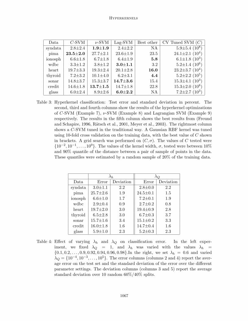
From Table 3, we observe that our method achieves state of the art results for all thedatasets, except the “heart” dataset. We also achieve results much better than previouslyreported for the “credit” dataset. Comparing the results for C-SVM and Tuned SVM,we observe that our method is always equally good, or better than a C-SVM tuned using10-fold cross validation.
7.3 Effect of λQ and λh on Classification Error
In order to investigate the effect of varying the hyperkernel regularization constant, λQ,and the Harmonic Hyperkernel parameter, λh, we performed experiments using the C-SVMhyperkernel optimization (Example 7). We performed two sets of experiments with each ofour chosen datasets. The results shown in Table 4.
From Table 4, we observe that the variation in classification accuracy over the wholerange of the hyperkernel regularization constant, λQ is less than the standard deviation ofthe classification accuracies of the various datasets (compare with Table 3). This demon-strates that our method is quite insensitive to the regularization parameter over the rangeof values tested for the various datasets.
The method shows a higher sensitivity to the harmonic hyperkernel parameter. Sincethis parameter effectively selects the scale of the problem, by selecting the “width” of thekernel, it is to be expected that each dataset would have a different ideal value of λh. It isto be noted that the generalization accuracy at λh = 0.6 is within one standard deviation(see Table 3 and 4) of the best accuracy achieved over the whole range tested.
1. We classified window vs. non-window for glass data, the other datasets are all binary.
1066
Hyperkernels
Data C-SVM ν-SVM Lag-SVM Best other CV Tuned SVM (C)syndata 2.8±2.4 1.9±1.9 2.4±2.2 NA 5.9±5.4 (108)pima 23.5±2.0 27.7±2.1 23.6±1.9 23.5 24.1±2.1 (104)
ionosph 6.6±1.8 6.7±1.8 6.4±1.9 5.8 6.1±1.8 (103)wdbc 3.3±1.2 3.8±1.2 3.0±1.1 3.2 5.2±1.4 (106)heart 19.7±3.3 19.3±2.4 20.1±2.8 16.0 23.2±3.7 (104)
thyroid 7.2±3.2 10.1±4.0 6.2±3.1 4.4 5.2±2.2 (105)sonar 14.8±3.7 15.3±3.7 14.7±3.6 15.4 15.3±4.1 (103)credit 14.6±1.8 13.7±1.5 14.7±1.8 22.8 15.3±2.0 (108)glass 6.0±2.4 8.9±2.6 6.0±2.2 NA 7.2±2.7 (103)
Table 3: Hyperkernel classification: Test error and standard deviation in percent. Thesecond, third and fourth columns show the results of the hyperkernel optimizationsof C-SVM (Example 7), ν-SVM (Example 8) and Lagrangian SVM (Example 9)respectively. The results in the fifth column shows the best results from (Freundand Schapire, 1996, Ratsch et al., 2001, Meyer et al., 2003). The rightmost columnshows a C-SVM tuned in the traditional way. A Gaussian RBF kernel was tunedusing 10-fold cross validation on the training data, with the best value of C shownin brackets. A grid search was performed on (C, σ). The values of C tested were10−2, 10−1, . . . , 109. The values of the kernel width, σ, tested were between 10%and 90% quantile of the distance between a pair of sample of points in the data.These quantiles were estimated by a random sample of 20% of the training data.
λh λQ
Data Error Deviation Error Deviationsyndata 3.0±1.1 2.2 2.8±0.0 2.2pima 25.7±2.6 1.9 24.5±0.1 1.5
ionosph 6.6±1.0 1.7 7.2±0.1 1.9wdbc 2.9±0.4 0.9 2.7±0.2 0.8heart 19.7±2.0 3.0 19.4±0.9 2.8
thyroid 6.5±2.8 3.0 6.7±0.3 3.7sonar 15.7±1.6 3.4 15.1±0.2 3.3credit 16.0±1.8 1.6 14.7±0.4 1.6glass 5.9±1.0 2.3 5.2±0.3 2.3
Table 4: Effect of varying λh and λQ on classification error. In the left exper-iment, we fixed λQ = 1, and λh was varied with the values λh =0.1, 0.2, . . . , 0.9, 0.92, 0.94, 0.96, 0.98.In the right, we set λh = 0.6 and variedλQ = 10−4, 10−3, . . . , 105. The error columns (columns 2 and 4) report the aver-age error on the test set and the standard deviation of the error over the differentparameter settings. The deviation columns (columns 3 and 5) report the averagestandard deviation over 10 random 60%/40% splits.
1067
Ong, Smola and Williamson
7.4 Computational Time
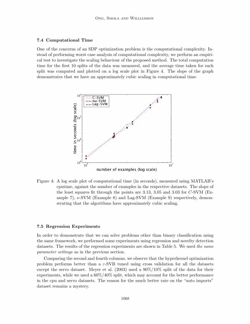
One of the concerns of an SDP optimization problem is the computational complexity. In-stead of performing worst case analysis of computational complexity, we perform an empiri-cal test to investigate the scaling behaviour of the proposed method. The total computationtime for the first 10 splits of the data was measured, and the average time taken for eachsplit was computed and plotted on a log scale plot in Figure 4. The slope of the graphdemonstrates that we have an approximately cubic scaling in computational time.
Figure 4: A log scale plot of computational time (in seconds), measured using MATLAB’scputime, against the number of examples in the respective datasets. The slope ofthe least squares fit through the points are 3.13, 3.05 and 3.03 for C-SVM (Ex-ample 7), ν-SVM (Example 8) and Lag-SVM (Example 9) respectively, demon-strating that the algorithms have approximately cubic scaling.
7.5 Regression Experiments
In order to demonstrate that we can solve problems other than binary classification usingthe same framework, we performed some experiments using regression and novelty detectiondatasets. The results of the regression experiments are shown in Table 5. We used the sameparameter settings as in the previous section.
Comparing the second and fourth columns, we observe that the hyperkernel optimizationproblem performs better than a ε-SVR tuned using cross validation for all the datasetsexcept the servo dataset. Meyer et al. (2003) used a 90%/10% split of the data for theirexperiments, while we used a 60%/40% split, which may account for the better performancein the cpu and servo datasets. The reason for the much better rate on the “auto imports”dataset remains a mystery.
1068

Hyperkernels
Data ν-SVR Best other CV Tuned ε-SVRauto-mpg 7.83±0.96 7.11 9.47±1.55boston 12.96±3.38 9.60 15.78±4.30
auto imports(×106) 5.91±2.41 0.25 7.51±5.33cpu(×103) 4.41±3.64 3.16 12.02±20.73
servo 0.74±0.26 0.25 0.62±0.25
Table 5: Hyperkernel regression: Mean Squared Error. The second column shows the re-sults from the hyperkernel optimization of the ν-regression (Example (11)). Theresults in the third column shows the best results from (Meyer et al., 2003). Therightmost column shows a ε-SVR with a gaussian kernel tuned using 10-fold crossvalidation on the training data. Similar to the classification setting, grid searchwas performed on (C, σ). The values of C tested were 10−2, 10−1, . . . , 109. Thevalues of the kernel width, σ, tested were between the 10% and 90% quantiles ofthe distance between a pair of sample of points in the data. These quantiles wereestimated by a random 20% sample of the training data.
7.6 Novelty Detection
We applied the single class support vector machine to detect outliers in the USPS data. Thetest set of the default split in the USPS database was used in the following experiments.The parameter ν was set to 0.1 for these experiments, hence selecting up to 10% of the dataas outliers.
Figure 5: Top rows: Images of digits ‘1’ and ‘2’, considered novel by algorithm; Bottom:typical images of digits ‘1’ and ‘2’.
Since there is no quantitative method for measuring the performance of novelty detec-tion, we cannot directly compare our results with the traditional single class SVM. We canonly subjectively conclude, by visually inspecting a sample of the digits, that our approachworks for novelty detection of USPS digits. Figure 5 shows a sample of the digits. We can
1069
Ong, Smola and Williamson
see that the algorithm identifies ‘novel’ digits, such as in the top two rows of Figure 5. Thebottom two rows shows a sample of digits which have been deemed to be ‘common’.
8. Summary and Outlook
The regularized quality functional allows the systematic solution of problems associated withthe choice of a kernel. Quality criteria that can be used include Kernel Target Alignment,regularized risk and the log posterior. The regularization implicit in our approach allowsthe control of overfitting that occurs if one optimizes over a too large a choice of kernels.
We have shown that when the empirical quality functional is the regularized risk func-tional, the resulting optimization problem is convex, and in fact is a SDP. This SDP, whichlearns the best kernel given the data, has a Bayesian interpretation in terms of a hierarchicalGaussian process. We define more general kernels which may have many free parameters,and optimize over them without overfitting. The experimental results on classificationdemonstrate that it is possible to achieve state of the art performance using our approachwith no manual tuning. Furthermore, the same framework and parameter settings work forvarious datasets as well as regression and novelty detection.
This approach makes support vector based estimation approaches more automated.Parameter adjustment is less critical compared to when the kernel is fixed, or hand tuned.Future work will focus on deriving improved statistical guarantees for estimates derived viahyperkernels which match the good empirical performance.
Acknowledgements The authors would like to thank Stephane Canu, Laurent El Ghaoui,Michael Jordan, John Lloyd, Daniela Pucci de Farias, Matthias Seeger, Grace Wahba andthe referees for their helpful comments and suggestions. The authors also thank AlexandrosKaratzoglou for his help with SVLAB. National ICT Australia is funded through the Aus-tralian Government’s Backing Australia’s Ability initiative, in part through the AustralianResearch Council.
References
A. Albert. Conditions for positive and nonnegative definiteness in terms of pseudoinverses.SIAM Journal on Applied Mathematics, 17(2):434 – 440, 1969.
N. Aronszajn. Theory of reproducing kernels. Transactions of the American MathematicalSociety, 68:337 – 404, 1950.
F. R. Bach and M. I. Jordan. Kernel independent component analysis. Journal of MachineLearning Research, 3:1 – 48, 2002.
K. P. Bennett and O. L. Mangasarian. Robust linear programming discrimination of twolinearly inseparable sets. Optimization Methods and Software, 1:23 – 34, 1992.
C. M. Bishop. Neural Networks for Pattern Recognition. Clarendon Press, Oxford, 1995.
O. Bousquet and D. Herrmann. On the complexity of learning the kernel matrix. InAdvances in Neural Information Processing Systems 15, pages 399–406, 2002.
1070
Hyperkernels
C. J. C. Burges. A tutorial on support vector machines for pattern recognition. Data Miningand Knowledge Discovery, 2(2):121 – 167, 1998.
O. Chapelle, V. Vapnik, O. Bousquet, and S. Mukherjee. Choosing multiple parameters forsupport vector machines. Machine Learning, 46(1):131 – 159, 2002.
C. Cortes and V. Vapnik. Support vector networks. Machine Learning, 20:273 – 297, 1995.
D. Cox and F. O’Sullivan. Asymptotic analysis of penalized likelihood and related estima-tors. Annals of Statistics, 18:1676 – 1695, 1990.
K. Crammer, J. Keshet, and Y. Singer. Kernel design using boosting. In Advances in NeuralInformation Processing Systems 15, pages 537–544, 2002.
N. Cristianini, J. Shawe-Taylor, A. Elisseeff, and J. Kandola. On kernel-target alignment. InT. G. Dietterich, S. Becker, and Z. Ghahramani, editors, Advances in Neural InformationProcessing Systems 14, pages 367 – 373, Cambridge, MA, 2002. MIT Press.
N. Cristianini, J. Kandola, A. Elisseeff, and J. Shawe-Taylor. On optimizing kernel align-ment. Technical report, UC Davis Department of Statistics, 2003.
K. Duan, S.S. Keerthi, and A.N. Poo. Evaluation of simple performance measures for tuningsvm hyperparameters. Neurocomputing, 51:41 – 59, 2003.
S. Fine and K. Scheinberg. Efficient SVM training using low-rank kernel representations.Journal of Machine Learning Research, 2:243 – 264, Dec 2001. http://www.jmlr.org.
Y. Freund and R. E. Schapire. Experiments with a new boosting algorithm. In Proceedingsof the International Conference on Machine Learing, pages 148 – 146. Morgan KaufmannPublishers, 1996.
D. Haussler. Convolutional kernels on discrete structures. Technical Report UCSC-CRL-99- 10, Computer Science Department, UC Santa Cruz, 1999.
R. Herbrich and R.C. Williamson. Algorithmic luckiness. Journal of Machine LearningResearch, 3:175 – 212, 2002.
G. S. Kimeldorf and G. Wahba. Some results on Tchebycheffian spline functions.J. Math. Anal. Applic., 33:82 – 95, 1971.
G. Lanckriet, N. Cristianini, P. Bartlett, L. El Ghaoui, and M. Jordan. Learning the kernelmatrix with semidefinite programming. In Proceedings of the International Conferenceon Machine Learning, pages 323–330. Morgan Kaufmann, 2002.
G. Lanckriet, N. Cristianini, P. Bartlett, L. El Ghaoui, and M. I. Jordan. Learning thekernel matrix with semi-definite programming. Journal of Machine Learning Research,5:27 – 72, 2004.
S. L. Lauritzen. Graphical Models. Oxford University Press, 1996.
1071
Ong, Smola and Williamson
J. Lofberg. YALMIP, yet another LMI parser, 2002. http://www.control.isy.liu.se/ ˜jo-hanl/yalmip.html.
A. Luntz and V. Brailovsky. On estimation of characters obtained in statistical procedureof recognition (in Russian). Technicheskaya Kibernetica, 3, 1969.
D. J. C. MacKay. Bayesian non-linear modelling for the energy prediction competition.ASHRAE Transcations, 4:448 – 472, 1994.
O. L. Mangasarian and D. R. Musicant. Lagrangian support vector machines. Journal ofMachine Learning Research, 1:161 – 177, 2001.
D. Meyer, F. Leisch, and K. Hornik. The support vector machine under test. Neurocom-puting, 55(1–2):169–186, 2003.
R. Neal. Bayesian Learning in Neural Networks. Springer, 1996.
C. S. Ong and A. J. Smola. Machine learning using hyperkernels. In Proceedings of theInternational Conference on Machine Learning, pages 568–575, 2003.
C. S. Ong, A. J. Smola, and R. C. Williamson. Hyperkernels. In Neural InformationProcessing Systems, volume 15, pages 495–502. MIT Press, 2002.
M. Opper and O. Winther. Gaussian processes and SVM: Mean field and leave-one-out. InA. J. Smola, P. L. Bartlett, B. Scholkopf, and D. Schuurmans, editors, Advances in LargeMargin Classifiers, pages 311 – 326, Cambridge, MA, 2000. MIT Press.
G. Ratsch, T. Onoda, and K. R. Muller. Soft margins for adaboost. Machine Learning, 42(3):287 – 320, 2001.
B. Scholkopf and A. J. Smola. Learning with Kernels. MIT Press, 2002.
B. Scholkopf, A. J. Smola, R. C. Williamson, and P. L. Bartlett. New support vectoralgorithms. Neural Computation, 12:1207 – 1245, 2000.
B. Scholkopf, J. Platt, J. Shawe-Taylor, A. J. Smola, and R. C. Williamson. Estimating thesupport of a high-dimensional distribution. Neural Computation, 13(7):1443–1471, 2001.
M. Seeger. Bayesian methods for support vector machines and Gaussian processes. Master’sthesis, University of Edinburgh, Division of Informatics, 1999.
A. J. Smola, B. Scholkopf, and K.-R. Muller. The connection between regularization oper-ators and support vector kernels. Neural Networks, 11(5):637 – 649, 1998.
J. F. Sturm. Using SeDuMi 1.02, a MATLAB toolbox for optimization over symmetriccones. Optimization Methods and Software, 11/12(1 - 4):625 – 653, 1999.
K. Tsuda, S. Akaho, and K. Asai. The EM algorithm for kernel matrix completion withauxiliary data. Journal of Machine Learning Research, 4:67–81, 2003.
L. Vandenberghe and S. Boyd. Semidefinite programming. SIAM Review., 38(1):49 – 95,1996.
1072
Hyperkernels
V. Vapnik. The Nature of Statistical Learning Theory. Springer, New York, 1995.
G. Wahba. Spline Models for Observational Data, volume 59 of CBMS-NSF Regional Con-ference Series in Applied Mathematics. SIAM, Philadelphia, 1990.
C. K. I. Williams and C. E. Rasmussen. Gaussian processes for regression. In D. S. Touret-zky, M. C. Mozer, and M. E. Hasselmo, editors, Advances in Neural Information Process-ing Systems 8, pages 514 – 520, Cambridge, MA, 1996. MIT Press.
Christopher K. I. Williams and David Barber. Bayesian classification with Gaussian pro-cesses. IEEE Transactions on Pattern Analysis and Machine Intelligence PAMI, 20(12):1342 – 1351, 1998.
T. Zhang. Some sparse approximation bounds for regression problems. In Proc. 18thInternational Conf. on Machine Learning, pages 624 – 631. Morgan Kaufmann, SanFrancisco, CA, 2001.
1073