Learning Real-Time Perspective Patch Rectiﬁcationcampar.in.tum.de/pub/hinterstoisser2011ijcv/hinterstoisser2011ijcv.pdf · Learning Real-Time Perspective Patch Rectiﬁcation

Noname manuscript No.(will be inserted by the editor)

Learning Real-Time Perspective Patch Rectification

Stefan Hinterstoisser · Vincent Lepetit · Selim Benhimane · Pascal Fua · NassirNavab

Received: date / Accepted: date

Abstract We propose two learning-based methods to patchrectification that are faster and more reliable than state-of-the-art affine region detection methods. Given a referenceview of a patch, they can quickly recognize it in new viewsand accurately estimate the homography between the refer-ence view and the new view. Our methods are more memory-consuming than affine region detectors, and are in practicecurrently limited to a few ten patches. However, if the refer-ence image is a fronto-parallel view and the internal param-eters known, one single patch is often enough to preciselyestimate an object pose. As a result, we can deal in real-timewith objects that are significantly less textured than the onesrequired by state-of-the-art methods.

The first method favors fast run-time performance whilethe second one is designed for fast real-time learning androbustness, however they follow the same general approach:First, a classifier provides for every keypoint a first estimateof its transformation. Then, the estimate allows carrying outan accurate perspective rectification using linear predictors.The last step is a fast verification—made possible by the ac-curate perspective rectification—of the patch identity anditssub-pixel precision position estimation. We demonstrate the

Stefan Hinterstoisser, Selim Benhimane, Nassir NavabComputer Aided Medical Procedures (CAMP)Technische Universitat Munchen (TUM)Boltzmannstrasse 3, 85748 Munich, GermanyTel.: +49-89-28919400Fax: +49-89-28917059E-mail:{hinterst,benhiman,navab}@in.tum.de

Vincent Lepetit, Pascal FuaComputer Vision Laboratory (CVLab)Ecole Polytechnique Federale de Lausanne (EPFL)CH-1015 Lausanne, SwitzerlandTel.: +41-21-6936716Fax: +41-21-6937520E-mail:{pascal.fua,vincent.lepetit}@epfl.ch

advantages of our approach on real-time 3D object detectionand tracking applications.

Keywords Patch Rectification· Tracking by Detection·Object Recognition· Online Learning· Real-TimeLearning· Pose Estimation

1 Introduction

Retrieving the poses of patches around keypoints in additionto matching them is an essential task in many applicationssuch as vision-based robot localization [9], object recogni-tion [25] or image retrieval [8,24] to constrain the problemat hand. It is usually done by decoupling the matching pro-cess from the keypoint pose estimation: The standard ap-proach is to first use some affine region detector [19] andthen rely on SIFT [15] or SURF [3] descriptors on the recti-fied regions to match them.

Recently, it has been shown that taking advantage of atraining phase, when possible, greatly improves the speedand the rate of keypoint recognition tasks [16,22]. Such atraining phase is possible when the application relies on somedatabaseof keypoints, such as object detection or SLAM.By contrast with [19], these learning-based approaches usu-ally do not rely on the extraction of local patch transforma-tions in order to handle larger perspective distortions butonthe ability to generalize well from training data. The draw-back is they only provide a 2–D location, while using anaffine region detector provides additional constraints thatproved to be useful [25,8].

To overcome this problem we introduce an approach il-lustrated in Fig. 1 and that can provide not only an affinetransformation but the full perspective patch rectification andthat is still real-time thanks to a learning stage. We show thisis very useful for object detection and SLAM applications:Applying our approach on a single keypoint is often enough

2

(a) (b) (c)

(d) (e) (f)

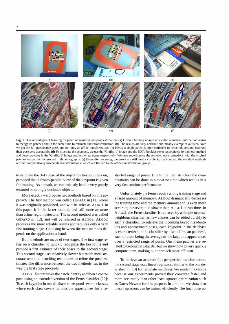
Fig. 1 The advantages of learning for patch recognition and pose estimation.(a) Given a training images or a video sequence, our method learnsto recognize patches and in the same time to estimate their transformation.(b) The results are very accurate and mostly exempt of outliers.Notewe get the full perspective pose, and not only an affine transformation.(c) Hence a single patch is often sufficient to detect objects andestimatetheir pose very accurately.(d) To illustrate the accuracy, we use the ’Graffiti 1’ image and the ICCV booklet cover respectively to train our methodand detect patches in the ’Graffiti 6’ image and in the real scene respectively. We then superimpose the retrieved transformations with the originalpatches warped by the ground truth homography.(e) Even after zooming, the errors are still barely visible.(f) By contrast, the standard methodsretrieve comparatively inaccurate transformations, which are limited to the affine transformation group.

to estimate the 3–D pose of the object the keypoint lies on,provided that a fronto-parallel view of the keypoint is givenfor training. As a result, we can robustly handle very poorlytextured or strongly occluded objects.

More exactly we propose two methods based on this ap-proach. The first method was called LEOPAR in [11] whereit was originally published, and will be refer as ALGO1 inthis paper. It is the faster method, and still more accuratethan affine region detectors. The second method was calledGEPARD in [12], and will be referred as ALGO2. ALGO2produces the more reliable results and requires only a veryfast training stage. Choosing between the two methods de-pends on the application at hand.

Both methods are made of two stages. The first stage re-lies on a classifier to quickly recognize the keypoints andprovide a first estimate of their poses to the second stage.This second stage uses relatively slower but much more ac-curate template matching techniques to refine the pose es-timate. The difference between the two methods lies in theway the first stage proceeds.

ALGO1 first retrieves the patch identity and then a coarsepose using an extended version of the Ferns classifier [22]:To each keypoint in our database correspond several classes,where each class covers its possible appearances for a re-

stricted range of poses. Due to the Fern structure the com-putations can be done in almost no time which results in avery fast runtime performance.

Unfortunately the Ferns require a long training stage anda large amount of memory. ALGO2 dramatically decreasesthe training time and the memory amount and is even moreaccurate; however, it is slower than ALGO1 at run-time. InALGO2, the Ferns classifier is replaced by a simple nearest-neighbour classifier, as new classes can be added quickly tosuch a classifier. To retrieve the incoming keypoints identi-ties and approximate poses, each keypoint in the databaseis characterized in the classifier by a set of “mean patches”,each of them being the average of the keypoint appearancesover a restricted range of poses. Our mean patches are re-lated to Geometric Blur [6], but we show how to very quicklycompute them, making our approach more efficient.

To retrieve an accurate full perspective transformation,the second stage uses linear regressors similar to the one de-scribed in [13] for template matching. We made this choicebecause our experiments proved they converge faster andmore accurately than other least-squares optimization suchas Gauss-Newton for this purpose. In addition, we show thatthese regressors can be trained efficiently The final pose es-

3

timate is typically accurate enough to allow a final check bysimple cross-correlation and prune the incorrect results.

Compared to affine region detectors, their closest com-petitors in the state-of-the-art, our two methods have one im-portant limitation: They do not scale very well with the sizeof the keypoints database, and our current limitations arelimited to a few tens of keypoints to keep real-time the appli-cations. Moreover, they need a frontal training view and thecamera internal parameters to compute the camera pose withrespect to the keypoint. However, as our experiments show,our two methods not only are much faster but they providean accurate 3–D pose for each keypoint, by contrast withan approximate affine transformation. In practice, a singlekeypoint is often enough to compute the camera or the tar-get pose, which compensates this limitation on the databasesize at least for the applications we present in this paper.

In the remainder of the paper, we first discuss relatedwork. Then, we describe our two methods, and comparethem against affine region detectors [19]. Finally, we presentapplications of tracking-by-detection and SLAM using ourmethod.

2 Related Work

Many different approaches often called “affine region de-tectors” have been proposed to recognize keypoints underlarge perspective distortion. For example, [27] generalizedthe Forstner-Harris approach, which was designed to de-tect keypoints stable under translation, to small similaritiesand affine transformations. However, it does not provide thetransformation itself. Other methods attempt to retrieve acanonical affine transformation withouta priori knowledge.This transformation is then used to rectify the image aroundthe keypoint and make them easier to recognize. For exam-ple, [19] showed that the Hessian-Affine detector of [18] andthe MSER detector of [17] are the most reliable ones. Inthe case of the Hessian-Affine detector, the retrieved affinetransformation is based on the image second moment ma-trix. It normalizes the region up to a rotation, which canthen be estimated for example by considering the peaks ofthe histogram of gradient orientations over the patch as inSIFT [15]. In the case of the MSER detector, other approachesexploiting the region shape are also possible [21], and acommon approach is to compute the transformation from theregion covariance matrix and solve for the remaining degreeof freedom using local maximums of curvature and bitan-gents.

But besides helping the recognition, the estimated affinetransformations can provide useful constraints. For example,[25] uses them to build and recognize 3–D objects in stereo-scopic images. [8] uses them to add constraints between thedifferent regions and help matching them more reliably.

Unfortunately, as the experiments presented in this papershow, the retrieved transformations are often not accurate.We will show that our learning-based methods can reach amuch better accuracy.

Learning-based methods to recognize keypoints becamequite popular recently, however all the previous methodsprovide only theidentity of the points, not their pose. Forexample, in [14], Randomized Trees are trained with ran-domly warped patches to estimate a probability distributionover the classes for each leaf node. The non-terminal nodescontain decisions based on pairwise intensity comparisonswhich are very fast to compute. Once the trees are trainedan incoming patch is classified by adding up the probabil-ity distributions of the leaf nodes that were reached and byidentifying the class with the maximal probability. However,training the Randomized Trees is slow and performed of-fline, which is problematic for applications such as SLAM.[28] replaced the Randomized Trees by a simpler list struc-ture and binary values instead of a probability distribution.These modifications allow them to learn new features onlinein real-time. Another approach based on the boosting algo-rithm presented in [10] to allow online feature learning inreal-time was proposed in [16].

More recently, [26] introduced a learning-based approachthat is closer to the approach presented in this paper. It isbased on what is called “Histogrammed Intensity Patches”(HIP). The link with our approach is that the HIPs are rem-iniscent of our “mean patches” used in ALGO2: Each key-point in the database is represented by a set of HIPs, eachof them computed over a small range of poses. For fast in-dexation, a HIP is a binarized histogram of the intensities ofa few pixels around the keypoint. However, while this is intheory possible, estimating the keypoint pose has not beenevaluated nor demonstrated, and this method too providesonly the keypoint identities.

Another work related to this paper is [20], which exploitsthe perspective transformation of patches centered on land-marks in a SLAM application. However, it is still very de-pending on the tracking prediction to match the landmarksand to retrieve their transformations, while we do not needany prior on the pose. Moreover, in [20], these transforma-tions are recovered using a Jacobian-based method while, inour case, a linear predictor can be trained very efficiently forfaster convergence.

In short, to the best of our knowledge, there is no methodin the literature that attempts to reach the exact same goal asours. Our two methods can estimate quickly and accuratelythe pose of keypoints of a database, thanks to a learning-based approach.

4

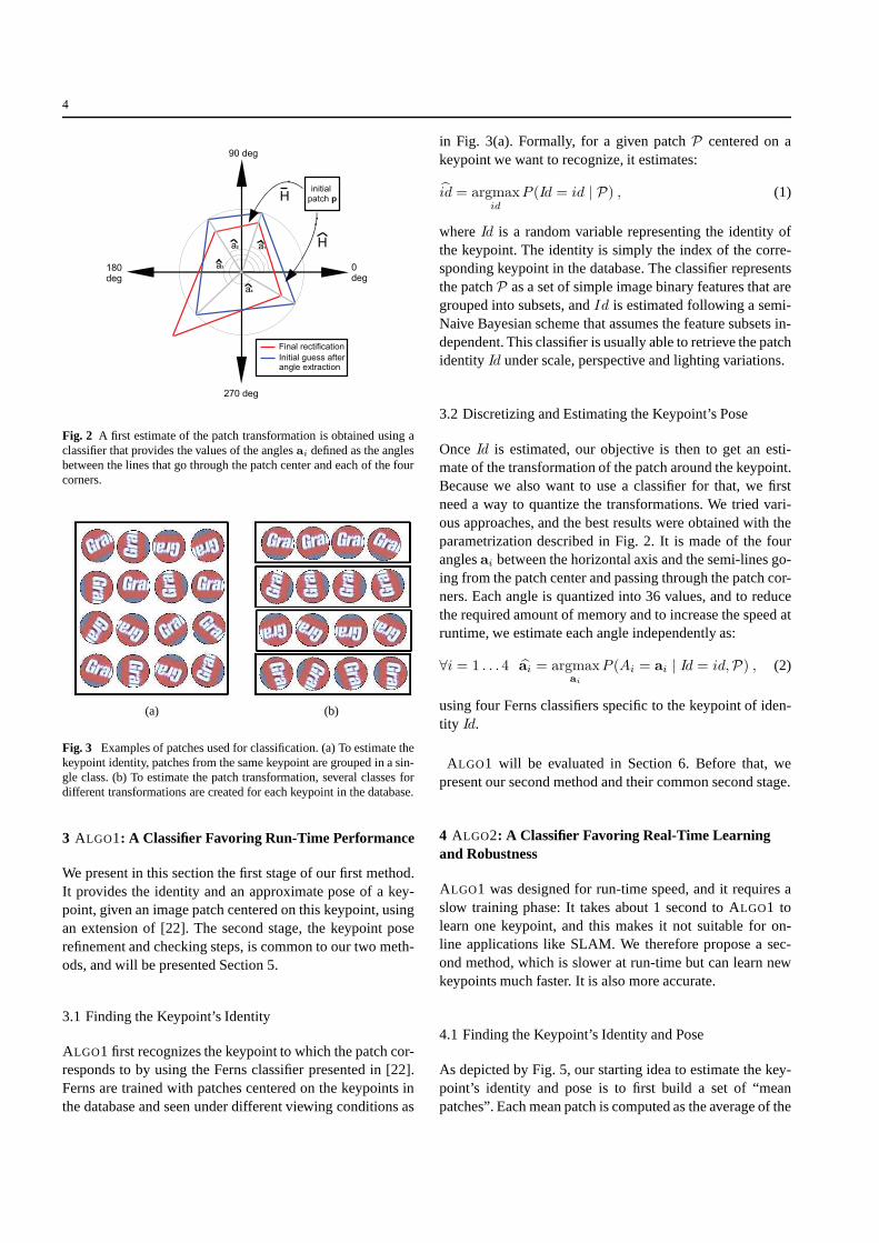
Fig. 2 A first estimate of the patch transformation is obtained using aclassifier that provides the values of the anglesai defined as the anglesbetween the lines that go through the patch center and each ofthe fourcorners.

(a) (b)

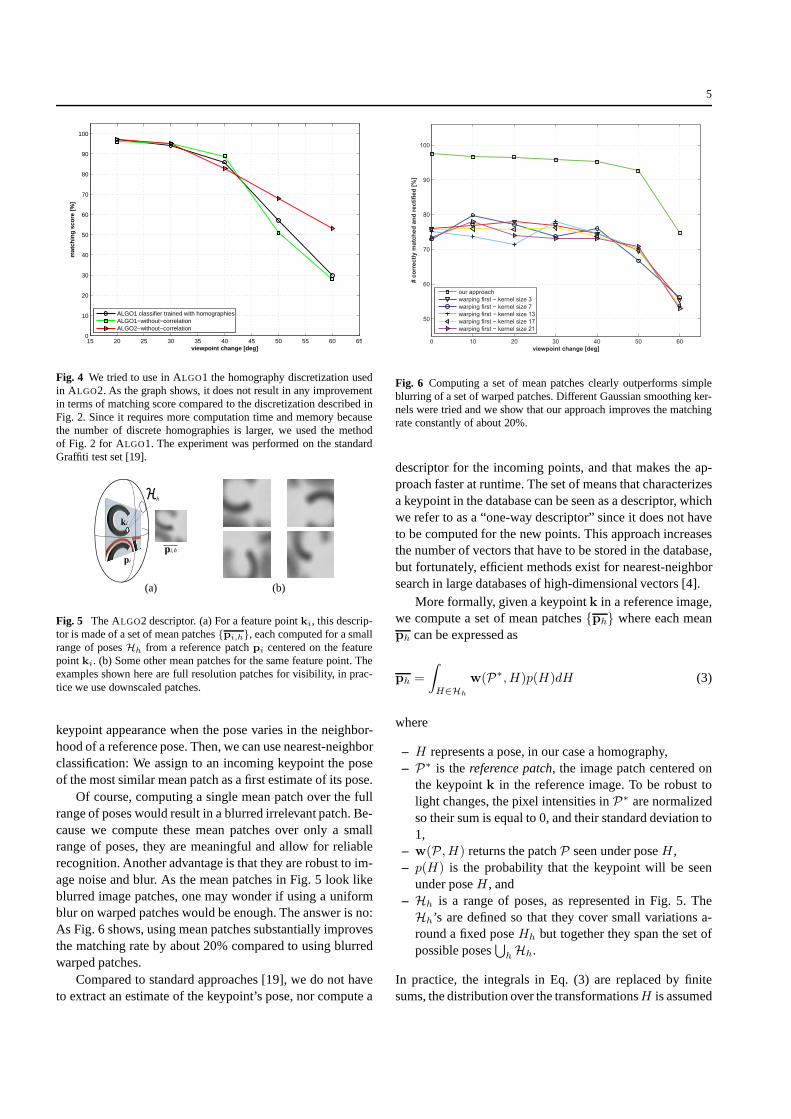
Fig. 3 Examples of patches used for classification. (a) To estimatethekeypoint identity, patches from the same keypoint are grouped in a sin-gle class. (b) To estimate the patch transformation, several classes fordifferent transformations are created for each keypoint inthe database.

3 ALGO1: A Classifier Favoring Run-Time Performance

We present in this section the first stage of our first method.It provides the identity and an approximate pose of a key-point, given an image patch centered on this keypoint, usingan extension of [22]. The second stage, the keypoint poserefinement and checking steps, is common to our two meth-ods, and will be presented Section 5.

3.1 Finding the Keypoint’s Identity

ALGO1 first recognizes the keypoint to which the patch cor-responds to by using the Ferns classifier presented in [22].Ferns are trained with patches centered on the keypoints inthe database and seen under different viewing conditions as

in Fig. 3(a). Formally, for a given patchP centered on akeypoint we want to recognize, it estimates:

id = argmaxid

P (Id = id | P) , (1)

whereId is a random variable representing the identity ofthe keypoint. The identity is simply the index of the corre-sponding keypoint in the database. The classifier representsthe patchP as a set of simple image binary features that aregrouped into subsets, andId is estimated following a semi-Naive Bayesian scheme that assumes the feature subsets in-dependent. This classifier is usually able to retrieve the patchidentityId under scale, perspective and lighting variations.

3.2 Discretizing and Estimating the Keypoint’s Pose

OnceId is estimated, our objective is then to get an esti-mate of the transformation of the patch around the keypoint.Because we also want to use a classifier for that, we firstneed a way to quantize the transformations. We tried vari-ous approaches, and the best results were obtained with theparametrization described in Fig. 2. It is made of the fouranglesai between the horizontal axis and the semi-lines go-ing from the patch center and passing through the patch cor-ners. Each angle is quantized into 36 values, and to reducethe required amount of memory and to increase the speed atruntime, we estimate each angle independently as:

∀i = 1 . . . 4 ai = argmaxai

P (Ai = ai | Id = id,P) , (2)

using four Ferns classifiers specific to the keypoint of iden-tity Id.

ALGO1 will be evaluated in Section 6. Before that, wepresent our second method and their common second stage.

4 ALGO2: A Classifier Favoring Real-Time Learningand Robustness

ALGO1 was designed for run-time speed, and it requires aslow training phase: It takes about 1 second to ALGO1 tolearn one keypoint, and this makes it not suitable for on-line applications like SLAM. We therefore propose a sec-ond method, which is slower at run-time but can learn newkeypoints much faster. It is also more accurate.

4.1 Finding the Keypoint’s Identity and Pose

As depicted by Fig. 5, our starting idea to estimate the key-point’s identity and pose is to first build a set of “meanpatches”. Each mean patch is computed as the average of the

5

15 20 25 30 35 40 45 50 55 60 650

10

20

30

40

50

60

70

80

90

100

viewpoint change [deg]

mat

chin

g s

core

[%

]

ALGO1 classifier trained with homographiesALGO1−without−correlationALGO2−without−correlation

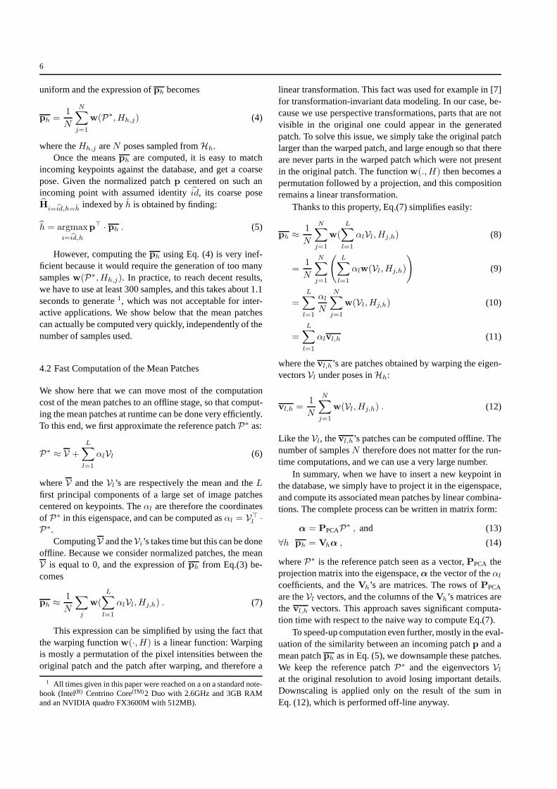
Fig. 4 We tried to use in ALGO1 the homography discretization usedin ALGO2. As the graph shows, it does not result in any improvementin terms of matching score compared to the discretization described inFig. 2. Since it requires more computation time and memory becausethe number of discrete homographies is larger, we used the methodof Fig. 2 for ALGO1. The experiment was performed on the standardGraffiti test set [19].

(a) (b)

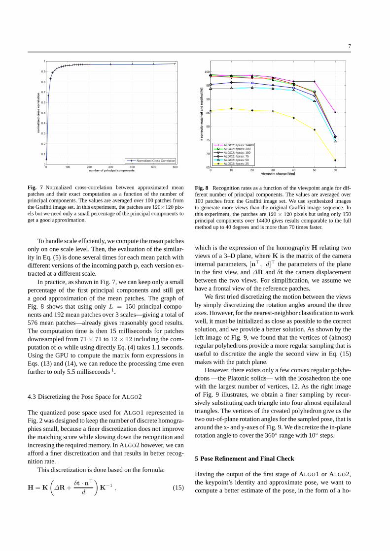
Fig. 5 The ALGO2 descriptor. (a) For a feature pointki, this descrip-tor is made of a set of mean patches{pi,h}, each computed for a smallrange of posesHh from a reference patchpi centered on the featurepointki. (b) Some other mean patches for the same feature point. Theexamples shown here are full resolution patches for visibility, in prac-tice we use downscaled patches.

keypoint appearance when the pose varies in the neighbor-hood of a reference pose. Then, we can use nearest-neighborclassification: We assign to an incoming keypoint the poseof the most similar mean patch as a first estimate of its pose.

Of course, computing a single mean patch over the fullrange of poses would result in a blurred irrelevant patch. Be-cause we compute these mean patches over only a smallrange of poses, they are meaningful and allow for reliablerecognition. Another advantage is that they are robust to im-age noise and blur. As the mean patches in Fig. 5 look likeblurred image patches, one may wonder if using a uniformblur on warped patches would be enough. The answer is no:As Fig. 6 shows, using mean patches substantially improvesthe matching rate by about 20% compared to using blurredwarped patches.

Compared to standard approaches [19], we do not haveto extract an estimate of the keypoint’s pose, nor compute a

0 10 20 30 40 50 60

50

60

70

80

90

100


# c

orr

ec

tly

ma

tch

ed

an

d r

ec

tifi

ed

[%

]

our approach

warping first − kernel size 3





Fig. 6 Computing a set of mean patches clearly outperforms simpleblurring of a set of warped patches. Different Gaussian smoothing ker-nels were tried and we show that our approach improves the matchingrate constantly of about 20%.

descriptor for the incoming points, and that makes the ap-proach faster at runtime. The set of means that characterizesa keypoint in the database can be seen as a descriptor, whichwe refer to as a “one-way descriptor” since it does not haveto be computed for the new points. This approach increasesthe number of vectors that have to be stored in the database,but fortunately, efficient methods exist for nearest-neighborsearch in large databases of high-dimensional vectors [4].

More formally, given a keypointk in a reference image,we compute a set of mean patches{ph} where each meanph can be expressed as

ph =

∫

H∈Hh

w(P∗, H)p(H)dH (3)

where

– H represents a pose, in our case a homography,– P∗ is thereference patch, the image patch centered on

the keypointk in the reference image. To be robust tolight changes, the pixel intensities inP∗ are normalizedso their sum is equal to 0, and their standard deviation to1,

– w(P , H) returns the patchP seen under poseH ,– p(H) is the probability that the keypoint will be seen

under poseH , and– Hh is a range of poses, as represented in Fig. 5. TheHh’s are defined so that they cover small variations a-round a fixed poseHh but together they span the set ofpossible poses

⋃hHh.

In practice, the integrals in Eq. (3) are replaced by finitesums, the distribution over the transformationsH is assumed

6

uniform and the expression ofph becomes

ph =1

N

N∑

j=1

w(P∗, Hh,j) (4)

where theHh,j areN poses sampled fromHh.Once the meansph are computed, it is easy to match

incoming keypoints against the database, and get a coarsepose. Given the normalized patchp centered on such anincoming point with assumed identityid, its coarse poseH

i=id,h=hindexed byh is obtained by finding:

h = argmaxi=id,h

p⊤ · ph . (5)

However, computing theph using Eq. (4) is very inef-ficient because it would require the generation of too manysamplesw(P∗, Hh,j). In practice, to reach decent results,we have to use at least 300 samples, and this takes about 1.1seconds to generate1, which was not acceptable for inter-active applications. We show below that the mean patchescan actually be computed very quickly, independently of thenumber of samples used.

4.2 Fast Computation of the Mean Patches

We show here that we can move most of the computationcost of the mean patches to an offline stage, so that comput-ing the mean patches at runtime can be done very efficiently.To this end, we first approximate the reference patchP∗ as:

P∗ ≈ V +

L∑

l=1

αlVl (6)

whereV and theVl’s are respectively the mean and theLfirst principal components of a large set of image patchescentered on keypoints. Theαl are therefore the coordinatesof P∗ in this eigenspace, and can be computed asαl = V

⊤l ·

P∗.ComputingV and theVi’s takes time but this can be done

offline. Because we consider normalized patches, the meanV is equal to 0, and the expression ofph from Eq.(3) be-comes

ph ≈1

N

∑

j

w(

L∑

l=1

αlVl, Hj,h) . (7)

This expression can be simplified by using the fact thatthe warping functionw(·, H) is a linear function: Warpingis mostly a permutation of the pixel intensities between theoriginal patch and the patch after warping, and therefore a

1 All times given in this paper were reached on a on a standard note-book (Intel(R) Centrino Core(TM)2 Duo with 2.6GHz and 3GB RAMand an NVIDIA quadro FX3600M with 512MB).

linear transformation. This fact was used for example in [7]for transformation-invariant data modeling. In our case, be-cause we use perspective transformations, parts that are notvisible in the original one could appear in the generatedpatch. To solve this issue, we simply take the original patchlarger than the warped patch, and large enough so that thereare never parts in the warped patch which were not presentin the original patch. The functionw(., H) then becomes apermutation followed by a projection, and this compositionremains a linear transformation.

Thanks to this property, Eq.(7) simplifies easily:

ph ≈1

N

N∑

j=1

w(

L∑

l=1

αlVl, Hj,h) (8)

=1

N

N∑

j=1

(L∑

l=1

αlw(Vl, Hj,h)

)(9)

=

L∑

l=1

αl

N

N∑

j=1

w(Vl, Hj,h) (10)

=

L∑

l=1

αlvl,h (11)

where thevl,h’s are patches obtained by warping the eigen-vectorsVl under poses inHh:

vl,h =1

N

N∑

j=1

w(Vl, Hj,h) . (12)

Like theVl, thevl,h’s patches can be computed offline. Thenumber of samplesN therefore does not matter for the run-time computations, and we can use a very large number.

In summary, when we have to insert a new keypoint inthe database, we simply have to project it in the eigenspace,and compute its associated mean patches by linear combina-tions. The complete process can be written in matrix form:

α = PPCAP∗ , and (13)

∀h ph = Vhα , (14)

whereP∗ is the reference patch seen as a vector,PPCA theprojection matrix into the eigenspace,α the vector of theαl

coefficients, and theVh’s are matrices. The rows ofPPCA

are theVl vectors, and the columns of theVh’s matrices arethevl,h vectors. This approach saves significant computa-tion time with respect to the naive way to compute Eq.(7).

To speed-up computation even further, mostly in the eval-uation of the similarity between an incoming patchp and amean patchph as in Eq. (5), we downsample these patches.We keep the reference patchP∗ and the eigenvectorsVlat the original resolution to avoid losing important details.Downscaling is applied only on the result of the sum inEq. (12), which is performed off-line anyway.

7

0 100 200 300 400 500 6000

0.1

0.2

0.3

0.4

0.5

0.6

0.7

0.8

0.9

1

number of principal components

no

rma

lize

d c

ros

s c

orr

ela

tio

n

Normalized Cross Correlation

Fig. 7 Normalized cross-correlation between approximated meanpatches and their exact computation as a function of the number ofprincipal components. The values are averaged over 100 patches fromthe Graffiti image set. In this experiment, the patches are120×120 pix-els but we need only a small percentage of the principal components toget a good approximation.

To handle scale efficiently, we compute the mean patchesonly on one scale level. Then, the evaluation of the similar-ity in Eq. (5) is done several times for each mean patch withdifferent versions of the incoming patchp, each version ex-tracted at a different scale.

In practice, as shown in Fig. 7, we can keep only a smallpercentage of the first principal components and still geta good approximation of the mean patches. The graph ofFig. 8 shows that using onlyL = 150 principal compo-nents and 192 mean patches over 3 scales—giving a total of576 mean patches—already gives reasonably good results.The computation time is then 15 milliseconds for patchesdownsampled from71 × 71 to 12 × 12 including the com-putation ofα while using directly Eq. (4) takes 1.1 seconds.Using the GPU to compute the matrix form expressions inEqs. (13) and (14), we can reduce the processing time evenfurther to only 5.5 milliseconds1.

4.3 Discretizing the Pose Space for ALGO2

The quantized pose space used for ALGO1 represented inFig. 2 was designed to keep the number of discrete homogra-phies small, because a finer discretization does not improvethe matching score while slowing down the recognition andincreasing the required memory. In ALGO2 however, we canafford a finer discretization and that results in better recog-nition rate.

This discretization is done based on the formula:

H = K

(∆R+

δt · n⊤

d

)K−1 , (15)

0 10 20 30 40 50 6065

70

75

80

85

90

95

100


# co

rrec

tly

mat

ched

an

d r

ecti

fied

[%

]

ALGO2: #pcas: 14400ALGO2: #pcas: 300ALGO2: #pcas: 150ALGO2: #pcas: 75ALGO2: #pcas: 50ALGO2: #pcas: 25

Fig. 8 Recognition rates as a function of the viewpoint angle for dif-ferent number of principal components. The values are averaged over100 patches from the Graffiti image set. We use synthesized imagesto generate more views than the original Graffiti image sequence. Inthis experiment, the patches are120 × 120 pixels but using only 150principal components over 14400 gives results comparable to the fullmethod up to 40 degrees and is more than 70 times faster.

which is the expression of the homographyH relating twoviews of a 3–D plane, whereK is the matrix of the camerainternal parameters,[n⊤, d]⊤ the parameters of the planein the first view, and∆R andδt the camera displacementbetween the two views. For simplification, we assume wehave a frontal view of the reference patches.

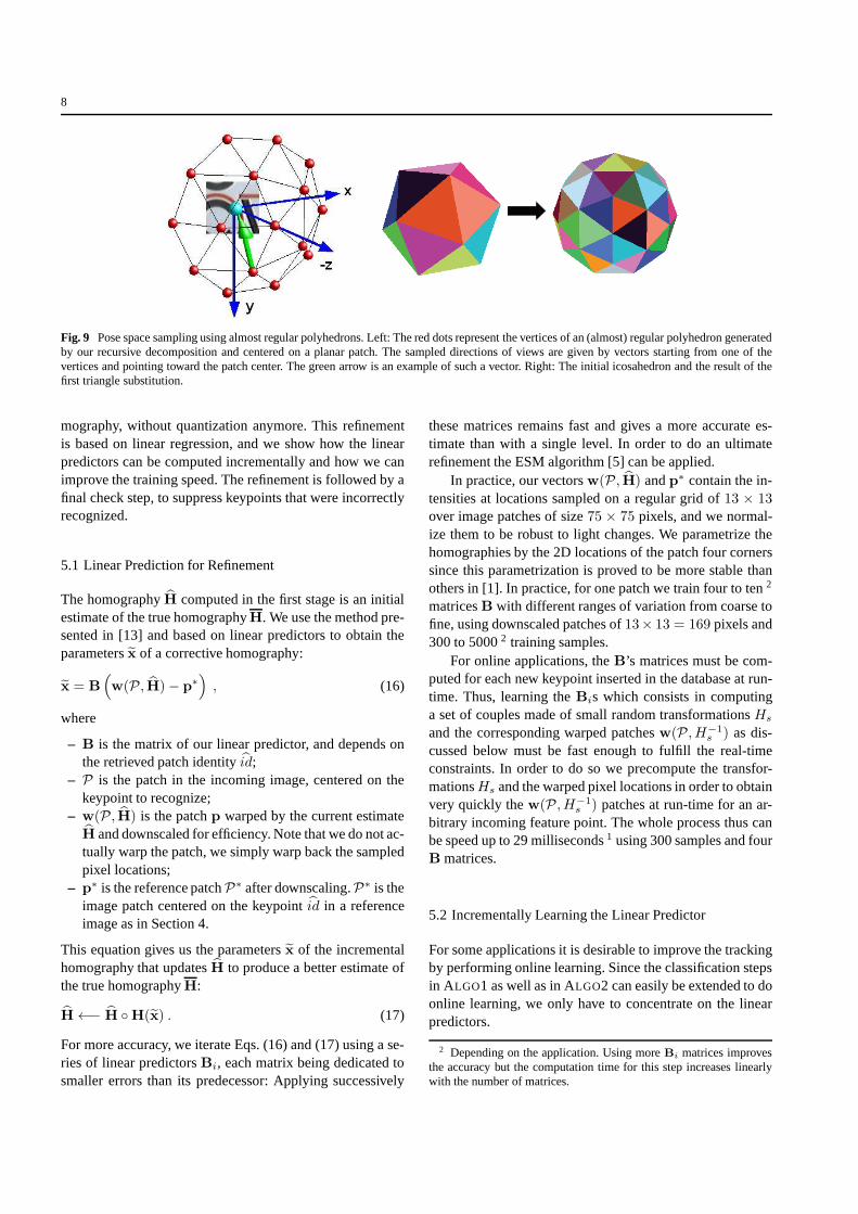
We first tried discretizing the motion between the viewsby simply discretizing the rotation angles around the threeaxes. However, for the nearest-neighbor classification to workwell, it must be initialized as close as possible to the correctsolution, and we provide a better solution. As shown by theleft image of Fig. 9, we found that the vertices of (almost)regular polyhedrons provide a more regular sampling that isuseful to discretize the angle the second view in Eq. (15)makes with the patch plane.

However, there exists only a few convex regular polyhe-drons —the Platonic solids— with the icosahedron the onewith the largest number of vertices, 12. As the right imageof Fig. 9 illustrates, we obtain a finer sampling by recur-sively substituting each triangle into four almost equilateraltriangles. The vertices of the created polyhedron give us thetwo out-of-plane rotation angles for the sampled pose, thatisaround the x- and y-axes of Fig. 9. We discretize the in-planerotation angle to cover the 360◦ range with 10◦ steps.

5 Pose Refinement and Final Check

Having the output of the first stage of ALGO1 or ALGO2,the keypoint’s identity and approximate pose, we want tocompute a better estimate of the pose, in the form of a ho-

8

Fig. 9 Pose space sampling using almost regular polyhedrons. Left: The red dots represent the vertices of an (almost) regular polyhedron generatedby our recursive decomposition and centered on a planar patch. The sampled directions of views are given by vectors starting from one of thevertices and pointing toward the patch center. The green arrow is an example of such a vector. Right: The initial icosahedron and the result of thefirst triangle substitution.

mography, without quantization anymore. This refinementis based on linear regression, and we show how the linearpredictors can be computed incrementally and how we canimprove the training speed. The refinement is followed by afinal check step, to suppress keypoints that were incorrectlyrecognized.

5.1 Linear Prediction for Refinement

The homographyH computed in the first stage is an initialestimate of the true homographyH. We use the method pre-sented in [13] and based on linear predictors to obtain theparametersx of a corrective homography:

x = B(w(P , H)− p∗

), (16)

where

– B is the matrix of our linear predictor, and depends onthe retrieved patch identityid;

– P is the patch in the incoming image, centered on thekeypoint to recognize;

– w(P , H) is the patchp warped by the current estimateH and downscaled for efficiency. Note that we do not ac-tually warp the patch, we simply warp back the sampledpixel locations;

– p∗ is the reference patchP∗ after downscaling.P∗ is theimage patch centered on the keypointid in a referenceimage as in Section 4.

This equation gives us the parametersx of the incrementalhomography that updatesH to produce a better estimate ofthe true homographyH:

H←− H ◦H(x) . (17)

For more accuracy, we iterate Eqs. (16) and (17) using a se-ries of linear predictorsBi, each matrix being dedicated tosmaller errors than its predecessor: Applying successively

these matrices remains fast and gives a more accurate es-timate than with a single level. In order to do an ultimaterefinement the ESM algorithm [5] can be applied.

In practice, our vectorsw(P , H) andp∗ contain the in-tensities at locations sampled on a regular grid of13 × 13over image patches of size75 × 75 pixels, and we normal-ize them to be robust to light changes. We parametrize thehomographies by the 2D locations of the patch four cornerssince this parametrization is proved to be more stable thanothers in [1]. In practice, for one patch we train four to ten2

matricesB with different ranges of variation from coarse tofine, using downscaled patches of13× 13 = 169 pixels and300 to 50002 training samples.

For online applications, theB’s matrices must be com-puted for each new keypoint inserted in the database at run-time. Thus, learning theBis which consists in computinga set of couples made of small random transformationsHs

and the corresponding warped patchesw(P , H−1s ) as dis-

cussed below must be fast enough to fulfill the real-timeconstraints. In order to do so we precompute the transfor-mationsHs and the warped pixel locations in order to obtainvery quickly thew(P , H−1

s ) patches at run-time for an ar-bitrary incoming feature point. The whole process thus canbe speed up to 29 milliseconds1 using 300 samples and fourB matrices.

5.2 Incrementally Learning the Linear Predictor

For some applications it is desirable to improve the trackingby performing online learning. Since the classification stepsin ALGO1 as well as in ALGO2 can easily be extended to doonline learning, we only have to concentrate on the linearpredictors.

2 Depending on the application. Using moreBi matrices improvesthe accuracy but the computation time for this step increases linearlywith the number of matrices.

9

The linear predictorB in Eq. (16) can be computed asthe pseudo-inverse of the analytically derived Jacobian ma-trix of a correlation measure [2,5]. However, the hyperplaneapproximation [13] computed from several examples yieldsa much larger region of convergence. The matrixB is thencomputed as:

B = XD⊤(DD⊤

)−1, (18)

whereX is a matrix made ofxi column vectors, andD amatrix made of column vectorsdi. Each vectordi is the dif-ference between the reference patchp∗ and the same patchafter warping by the homography parametrized byxi: di =

w(p,H(xi))− p∗.Eq. (18) requires all the couples(xi,di) to be simulta-

neously available. If it is applied directly, this preventsin-cremental learning but this can be fixed. Suppose that thematrix B = Bn is already computed forn examples, andthen a new example(xn+1,dn+1) becomes available. Wewant to update the matrixB into the matrixBn+1 that takesinto account all then + 1 examples. Let us introduce thematricesYn = XnD

⊤n andZn = DnD

⊤n . We then have:

Bn+1 = Yn+1Z−1

n+1

= Xn+1D⊤n+1

(Dn+1D

⊤n+1

)−1

= [Xn|xn+1][Dn|dn+1]⊤([Dn|dn+1][Dn|dn+1]

⊤)−1

=(XnD

⊤n + xn+1d

⊤n+1

) (DnD

⊤n + dn+1d

⊤n+1

)−1

=(Yn + xn+1d

⊤n+1

) (Zn + dn+1d

⊤n+1

)−1(19)

wherexn+1 anddn+1 are concatenated toXn andDn re-spectively to formXn+1 andDn+1. Thus, by only storingtheconstant sizematricesYn andZn and updating them as:

Yn+1 ←− Yn + xn+1d⊤n+1 (20)

Zn+1 ←− Zn + dn+1d⊤n+1 , (21)

it becomes possible to incrementally learn the linear predic-tor without storing the previous examples, and allows for anarbitrary large number of examples.

Since the computation ofB has to be done for manylocations in each incoming image andZn is a large ma-trix in practice, we need to go one step further in order toavoid the computation ofZ−1

n at every iteration. We applythe Sherman-Morrison formula toZ−1

n+1 and we get:

Z−1

n+1 =(Zn + dn+1d

⊤n+1

)−1

= Z−1n −

Z−1n dn+1d

⊤n+1Z

−1n

1 + d⊤n+1

Z−1n dn+1

. (22)

Therefore, if we storeZ−1n instead ofZn itself, and update

it using Eq. (22), no matrix inversion is required anymore,and the computation of matrixBn+1 becomes very fast.

5.3 Correlation-based Hypothesis Selection andVerification

In ALGO2, for each possible keypoint identityi, we usethe method explained above to estimate a fine homogra-phy Hi,final. Thanks to the high accuracy of the retrievedtransformation, we can select the correct pair of keypointidentity i and poseHi,final based on the normalized cross-correlation between the reference patchP∗

i and the warpedpatchw(P , Hi,final) seen under poseHi,final. The selectionis done by

argmaxi

P∗i⊤ ·w(P , Hi,final) , (23)

In ALGO1, the keypoint identityi is directly provided by theFerns classifier.

Finally, we use a thresholdτNCC = 0.9 in order to re-move wrong matches:

w(P , Hi,final)⊤ · P∗

i > τNCC , (24)

Thus, each patchw(P , Hi,final) that gives the maximum sim-ilarity score, which exceedsτNCC at the same time, yields anaccepted match.

6 Experimental Validation

We compare here our approach against affine region detec-tors on the Graffiti image set from [19] towards robustnessand accuracy. At the end of this section, we also evaluatethe performance of our algorithms with respect to trainingtime, running time and memory consumption. For each ex-periment we give a detailed discussion about the specific ad-vantages of each of our two methods.

6.1 Evaluation on the Graffiti Image Set

We first built a database of the most stable 100 Harris key-points from the first image of the Graffiti set. These key-points were found by synthetically rendering the image un-der many random transformations, adding artificial imagenoise and extracting Harris keypoints. We then kept the 100keypoints detected the most frequently.

The Ferns classifiers in ALGO1 were trained with syn-thetic images as well, by scaling and rotating the first imagefor changes in viewpoint angle up to 65 degrees and addingnoise. In the case of ALGO2 only the first image is needed.We then extracted Harris keypoints in the other images ofthe set, and run ALGO1 and ALGO2 to recognize them andestimate their poses.

We also run the different region detectors over the setimages and matched the regions in the first image againstthe regions in the other images using the SIFT descriptorcomputed on the rectified regions.

10

15 20 25 30 35 40 45 50 55 60 650

10

20

30

40

50

60

70

80

90

100


mat

chin

g s

core

[%

]

ALGO1−without−correlationALGO2−without−correlationHarris AffineHessian AffineMSERIBREBR

15 20 25 30 35 40 45 50 55 60 650

10

20

30

40

50

60

70

80

90

100


mat

chin

g s

core

[%

]

ALGO1

ALGO2

Harris Affine

Hessian Affine

MSER

IBR

EBR

(a) (b)

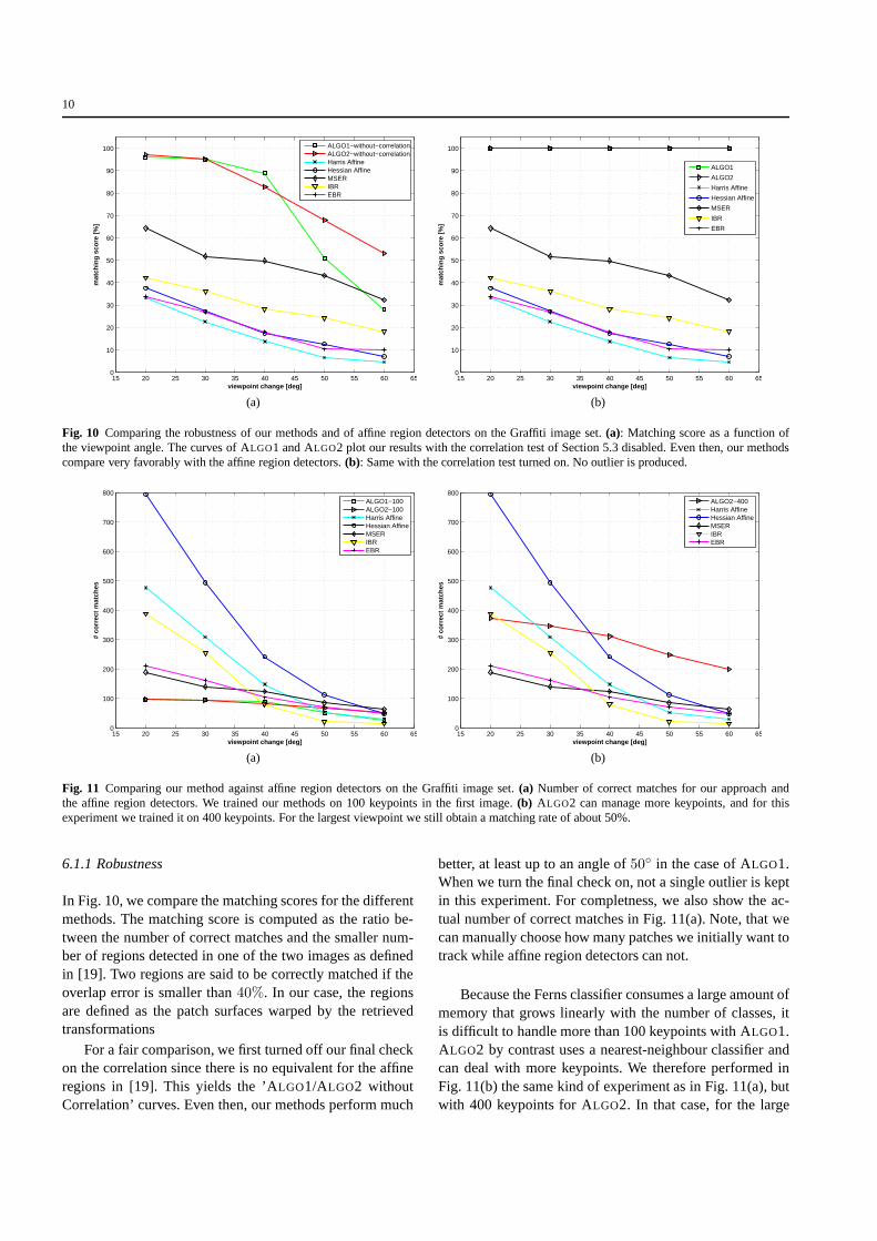
Fig. 10 Comparing the robustness of our methods and of affine region detectors on the Graffiti image set.(a): Matching score as a function ofthe viewpoint angle. The curves of ALGO1 and ALGO2 plot our results with the correlation test of Section 5.3 disabled. Even then, our methodscompare very favorably with the affine region detectors.(b): Same with the correlation test turned on. No outlier is produced.

15 20 25 30 35 40 45 50 55 60 650

100

200

300

400

500

600

700

800


# co

rrec

t m

atch

es

ALGO1−100ALGO2−100Harris AffineHessian AffineMSERIBREBR

15 20 25 30 35 40 45 50 55 60 650

100

200

300

400

500

600

700

800


# co

rrec

t m

atch

es

ALGO2−400Harris AffineHessian AffineMSERIBREBR

(a) (b)

Fig. 11 Comparing our method against affine region detectors on the Graffiti image set.(a) Number of correct matches for our approach andthe affine region detectors. We trained our methods on 100 keypoints in the first image.(b) ALGO2 can manage more keypoints, and for thisexperiment we trained it on 400 keypoints. For the largest viewpoint we still obtain a matching rate of about 50%.

6.1.1 Robustness

In Fig. 10, we compare the matching scores for the differentmethods. The matching score is computed as the ratio be-tween the number of correct matches and the smaller num-ber of regions detected in one of the two images as definedin [19]. Two regions are said to be correctly matched if theoverlap error is smaller than40%. In our case, the regionsare defined as the patch surfaces warped by the retrievedtransformations

For a fair comparison, we first turned off our final checkon the correlation since there is no equivalent for the affineregions in [19]. This yields the ’ALGO1/ALGO2 withoutCorrelation’ curves. Even then, our methods perform much

better, at least up to an angle of50◦ in the case of ALGO1.When we turn the final check on, not a single outlier is keptin this experiment. For completness, we also show the ac-tual number of correct matches in Fig. 11(a). Note, that wecan manually choose how many patches we initially want totrack while affine region detectors can not.

Because the Ferns classifier consumes a large amount ofmemory that grows linearly with the number of classes, itis difficult to handle more than 100 keypoints with ALGO1.ALGO2 by contrast uses a nearest-neighbour classifier andcan deal with more keypoints. We therefore performed inFig. 11(b) the same kind of experiment as in Fig. 11(a), butwith 400 keypoints for ALGO2. In that case, for the large

11

viewpoint angles, we get more correctly matches keypointsthan regions with the affine region detectors.

ALGO2 is also more robust to scale and perspective dis-tortions than ALGO1. In practice we found out that the limit-ing factor is by far the repeatability of the keypoint detector.However, once a keypoint is correctly detected, it is veryfrequently correctly matched at least by ALGO2.

6.1.2 2–D Accuracy

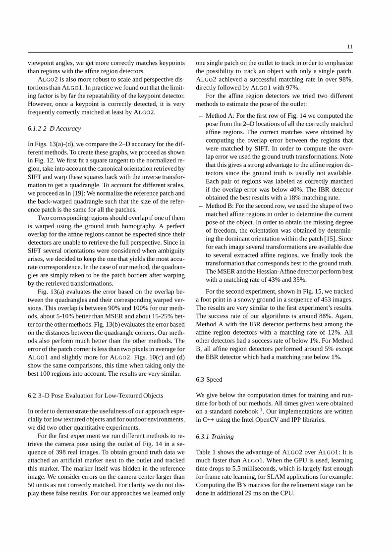
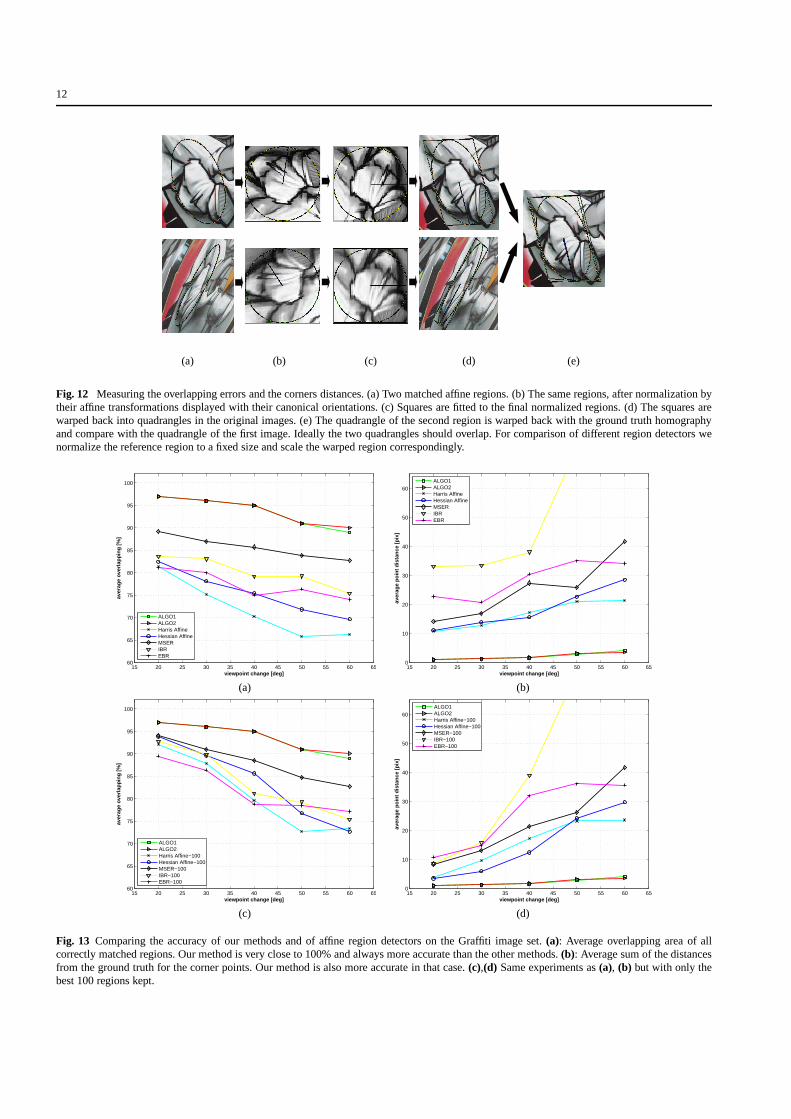
In Figs. 13(a)-(d), we compare the 2–D accuracy for the dif-ferent methods. To create these graphs, we proceed as shownin Fig. 12. We first fit a square tangent to the normalized re-gion, take into account the canonical orientation retrieved bySIFT and warp these squares back with the inverse transfor-mation to get a quadrangle. To account for different scales,we proceed as in [19]: We normalize the reference patch andthe back-warped quadrangle such that the size of the refer-ence patch is the same for all the patches.

Two corresponding regions should overlap if one of themis warped using the ground truth homography. A perfectoverlap for the affine regions cannot be expected since theirdetectors are unable to retrieve the full perspective. Since inSIFT several orientations were considered when ambiguityarises, we decided to keep the one that yields the most accu-rate correspondence. In the case of our method, the quadran-gles are simply taken to be the patch borders after warpingby the retrieved transformations.

Fig. 13(a) evaluates the error based on the overlap be-tween the quadrangles and their corresponding warped ver-sions. This overlap is between 90% and 100% for our meth-ods, about 5-10% better than MSER and about 15-25% bet-ter for the other methods. Fig. 13(b) evaluates the error basedon the distances between the quadrangle corners. Our meth-ods also perform much better than the other methods. Theerror of the patch corner is less than two pixels in average forALGO1 and slightly more for ALGO2. Figs. 10(c) and (d)show the same comparisons, this time when taking only thebest 100 regions into account. The results are very similar.

6.2 3–D Pose Evaluation for Low-Textured Objects

In order to demonstrate the usefulness of our approach espe-cially for low textured objects and for outdoor environments,we did two other quantitative experiments.

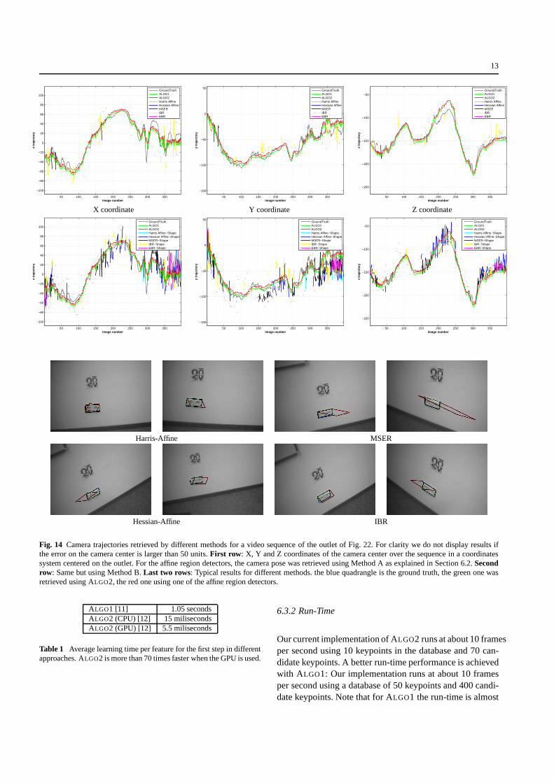
For the first experiment we run different methods to re-trieve the camera pose using the outlet of Fig. 14 in a se-quence of 398 real images. To obtain ground truth data weattached an artificial marker next to the outlet and trackedthis marker. The marker itself was hidden in the referenceimage. We consider errors on the camera center larger than50 units as not correctly matched. For clarity we do not dis-play these false results. For our approaches we learned only

one single patch on the outlet to track in order to emphasizethe possibility to track an object with only a single patch.ALGO2 achieved a successful matching rate in over 98%,directly followed by ALGO1 with 97%.

For the affine region detectors we tried two differentmethods to estimate the pose of the outlet:

– Method A: For the first row of Fig. 14 we computed thepose from the 2–D locations of all the correctly matchedaffine regions. The correct matches were obtained bycomputing the overlap error between the regions thatwere matched by SIFT. In order to compute the over-lap error we used the ground truth transformations. Notethat this gives a strong advantage to the affine region de-tectors since the ground truth is usually not available.Each pair of regions was labeled as correctly matchedif the overlap error was below 40%. The IBR detectorobtained the best results with a 18% matching rate.

– Method B: For the second row, we used the shape of twomatched affine regions in order to determine the currentpose of the object. In order to obtain the missing degreeof freedom, the orientation was obtained by determin-ing the dominant orientation within the patch [15]. Sincefor each image several transformations are available dueto several extracted affine regions, we finally took thetransformation that corresponds best to the ground truth.The MSER and the Hessian-Affine detector perform bestwith a matching rate of 43% and 35%.

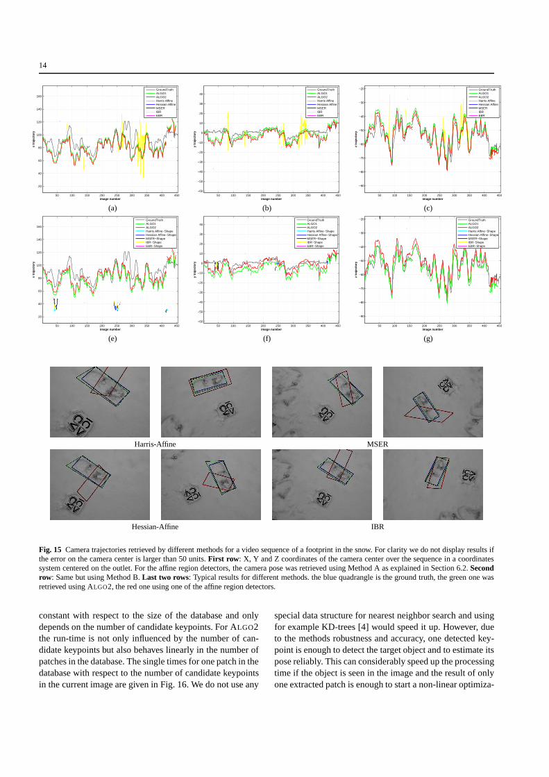
For the second experiment, shown in Fig. 15, we trackeda foot print in a snowy ground in a sequence of 453 images.The results are very similar to the first experiment’s results.The success rate of our algorithms is around 88%. Again,Method A with the IBR detector performs best among theaffine region detectors with a matching rate of 12%. Allother detectors had a success rate of below 1%. For MethodB, all affine region detectors performed around 5% exceptthe EBR detector which had a matching rate below 1%.

6.3 Speed

We give below the computation times for training and run-time for both of our methods. All times given were obtainedon a standard notebook1. Our implementations are writtenin C++ using the Intel OpenCV and IPP libraries.

6.3.1 Training

Table 1 shows the advantage of ALGO2 over ALGO1: It ismuch faster than ALGO1. When the GPU is used, learningtime drops to 5.5 milliseconds, which is largely fast enoughfor frame rate learning, for SLAM applications for example.Computing theB’s matrices for the refinement stage can bedone in additional 29 ms on the CPU.

12

(a) (b) (c) (d) (e)

Fig. 12 Measuring the overlapping errors and the corners distances. (a) Two matched affine regions. (b) The same regions, after normalization bytheir affine transformations displayed with their canonical orientations. (c) Squares are fitted to the final normalizedregions. (d) The squares arewarped back into quadrangles in the original images. (e) Thequadrangle of the second region is warped back with the ground truth homographyand compare with the quadrangle of the first image. Ideally the two quadrangles should overlap. For comparison of different region detectors wenormalize the reference region to a fixed size and scale the warped region correspondingly.

15 20 25 30 35 40 45 50 55 60 6560

65

70

75

80

85

90

95

100


aver

age

ove

rlap

pin

g [

%]

ALGO1ALGO2Harris AffineHessian AffineMSERIBREBR

15 20 25 30 35 40 45 50 55 60 650

10

20

30

40

50

60


aver

age

po

int

dis

tan

ce [

pix

]

ALGO1ALGO2Harris AffineHessian AffineMSERIBREBR

(a) (b)

15 20 25 30 35 40 45 50 55 60 6560

65

70

75

80

85

90

95

100


aver

age

ove

rlap

pin

g [

%]

ALGO1ALGO2Harris Affine−100Hessian Affine−100MSER−100IBR−100EBR−100

15 20 25 30 35 40 45 50 55 60 650

10

20

30

40

50

60


aver

age

po

int

dis

tan

ce [

pix

]

ALGO1ALGO2Harris Affine−100Hessian Affine−100MSER−100IBR−100EBR−100

(c) (d)

Fig. 13 Comparing the accuracy of our methods and of affine region detectors on the Graffiti image set.(a): Average overlapping area of allcorrectly matched regions. Our method is very close to 100% and always more accurate than the other methods.(b): Average sum of the distancesfrom the ground truth for the corner points. Our method is also more accurate in that case.(c),(d) Same experiments as(a), (b) but with only thebest 100 regions kept.

13

50 100 150 200 250 300 350

−100

−80

−60

−40

−20

0

20

40

60

80

100

image number

x tr

ajec

tory

GroundTruthALGO1ALGO2Harris AffineHessian AffineMSERIBREBR

50 100 150 200 250 300 350

−150

−100

−50

0

50

image number

y tr

ajec

tory


50 100 150 200 250 300 350

−250

−200

−150

−100

−50

image number

z tr

ajec

tory


X coordinate Y coordinate Z coordinate

50 100 150 200 250 300 350

−100

−80

−60

−40

−20

0

20

40

60

80

100

image number

x tr

ajec

tory

GroundTruthALGO1ALGO2Harris Affine−ShapeHessian Affine−ShapeMSER−ShapeIBR−ShapeEBR−Shape

50 100 150 200 250 300 350

−150

−100

−50

0

50

image number

y tr

ajec

tory


50 100 150 200 250 300 350

−250

−200

−150

−100

−50

image number

z tr

ajec

tory


Harris-Affine MSER

Hessian-Affine IBR

Fig. 14 Camera trajectories retrieved by different methods for a video sequence of the outlet of Fig. 22. For clarity we do not display results ifthe error on the camera center is larger than 50 units.First row : X, Y and Z coordinates of the camera center over the sequencein a coordinatessystem centered on the outlet. For the affine region detectors, the camera pose was retrieved using Method A as explained in Section 6.2.Secondrow: Same but using Method B.Last two rows: Typical results for different methods. the blue quadrangle is the ground truth, the green one wasretrieved using ALGO2, the red one using one of the affine region detectors.

ALGO1 [11] 1.05 secondsALGO2 (CPU) [12] 15 milisecondsALGO2 (GPU) [12] 5.5 miliseconds

Table 1 Average learning time per feature for the first step in differentapproaches. ALGO2 is more than 70 times faster when the GPU is used.

6.3.2 Run-Time

Our current implementation of ALGO2 runs at about 10 framesper second using 10 keypoints in the database and 70 can-didate keypoints. A better run-time performance is achievedwith ALGO1: Our implementation runs at about 10 framesper second using a database of 50 keypoints and 400 candi-date keypoints. Note that for ALGO1 the run-time is almost

14

50 100 150 200 250 300 350 400 450

20

40

60

80

100

120

140

160

image number

x tr

ajec

tory


50 100 150 200 250 300 350 400 450−60

−50

−40

−30

−20

−10

0

10

20

30

40

image number

y tr

ajec

tory


50 100 150 200 250 300 350 400 450

−90

−80

−70

−60

−50

−40

−30

−20

image number

z tr

ajec

tory


(a) (b) (c)

50 100 150 200 250 300 350 400 450

20

40

60

80

100

120

140

160

image number

x tr

ajec

tory


50 100 150 200 250 300 350 400 450−60

−50

−40

−30

−20

−10

0

10

20

30

40

image number

y tr

ajec

tory


50 100 150 200 250 300 350 400 450

−90

−80

−70

−60

−50

−40

−30

−20

image number

z tr

ajec

tory


(e) (f) (g)

Harris-Affine MSER

Hessian-Affine IBR

Fig. 15 Camera trajectories retrieved by different methods for a video sequence of a footprint in the snow. For clarity we do not display results ifthe error on the camera center is larger than 50 units.First row : X, Y and Z coordinates of the camera center over the sequencein a coordinatessystem centered on the outlet. For the affine region detectors, the camera pose was retrieved using Method A as explained in Section 6.2.Secondrow: Same but using Method B.Last two rows: Typical results for different methods. the blue quadrangle is the ground truth, the green one wasretrieved using ALGO2, the red one using one of the affine region detectors.

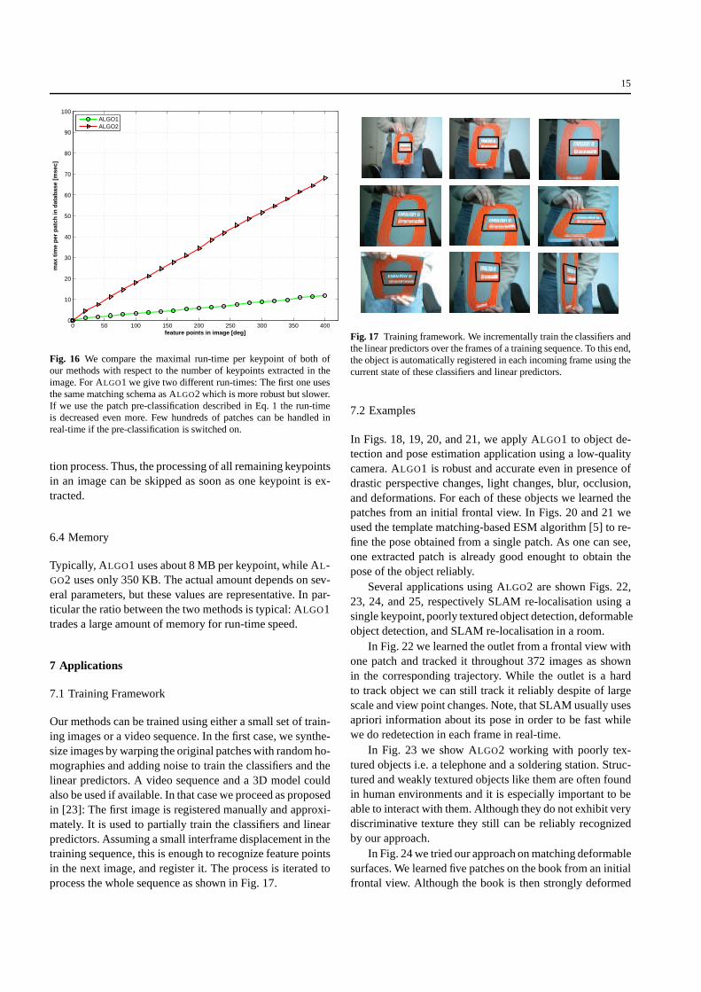
constant with respect to the size of the database and onlydepends on the number of candidate keypoints. For ALGO2the run-time is not only influenced by the number of can-didate keypoints but also behaves linearly in the number ofpatches in the database. The single times for one patch in thedatabase with respect to the number of candidate keypointsin the current image are given in Fig. 16. We do not use any

special data structure for nearest neighbor search and usingfor example KD-trees [4] would speed it up. However, dueto the methods robustness and accuracy, one detected key-point is enough to detect the target object and to estimate itspose reliably. This can considerably speed up the processingtime if the object is seen in the image and the result of onlyone extracted patch is enough to start a non-linear optimiza-

15

0 50 100 150 200 250 300 350 4000

10

20

30

40

50

60

70

80

90

100

feature points in image [deg]

max

tim

e p

er p

atch

in d

atab

ase

[mse

c]

ALGO1ALGO2

Fig. 16 We compare the maximal run-time per keypoint of both ofour methods with respect to the number of keypoints extracted in theimage. For ALGO1 we give two different run-times: The first one usesthe same matching schema as ALGO2 which is more robust but slower.If we use the patch pre-classification described in Eq. 1 the run-timeis decreased even more. Few hundreds of patches can be handled inreal-time if the pre-classification is switched on.

tion process. Thus, the processing of all remaining keypointsin an image can be skipped as soon as one keypoint is ex-tracted.

6.4 Memory

Typically, ALGO1 uses about 8 MB per keypoint, while AL-GO2 uses only 350 KB. The actual amount depends on sev-eral parameters, but these values are representative. In par-ticular the ratio between the two methods is typical: ALGO1trades a large amount of memory for run-time speed.

7 Applications

7.1 Training Framework

Our methods can be trained using either a small set of train-ing images or a video sequence. In the first case, we synthe-size images by warping the original patches with random ho-mographies and adding noise to train the classifiers and thelinear predictors. A video sequence and a 3D model couldalso be used if available. In that case we proceed as proposedin [23]: The first image is registered manually and approxi-mately. It is used to partially train the classifiers and linearpredictors. Assuming a small interframe displacement in thetraining sequence, this is enough to recognize feature pointsin the next image, and register it. The process is iterated toprocess the whole sequence as shown in Fig. 17.

Fig. 17 Training framework. We incrementally train the classifiersandthe linear predictors over the frames of a training sequence. To this end,the object is automatically registered in each incoming frame using thecurrent state of these classifiers and linear predictors.

7.2 Examples

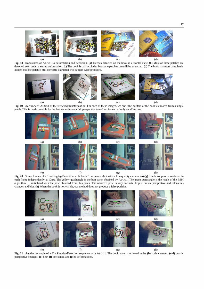
In Figs. 18, 19, 20, and 21, we apply ALGO1 to object de-tection and pose estimation application using a low-qualitycamera. ALGO1 is robust and accurate even in presence ofdrastic perspective changes, light changes, blur, occlusion,and deformations. For each of these objects we learned thepatches from an initial frontal view. In Figs. 20 and 21 weused the template matching-based ESM algorithm [5] to re-fine the pose obtained from a single patch. As one can see,one extracted patch is already good enought to obtain thepose of the object reliably.

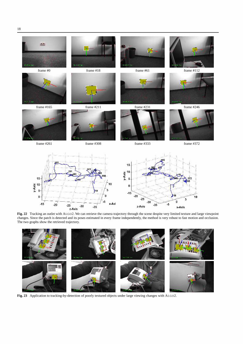
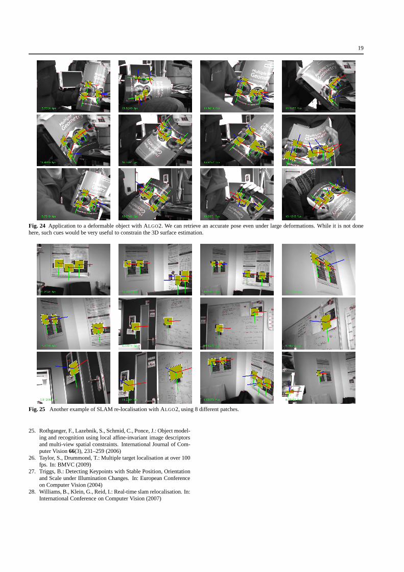
Several applications using ALGO2 are shown Figs. 22,23, 24, and 25, respectively SLAM re-localisation using asingle keypoint, poorly textured object detection, deformableobject detection, and SLAM re-localisation in a room.

In Fig. 22 we learned the outlet from a frontal view withone patch and tracked it throughout 372 images as shownin the corresponding trajectory. While the outlet is a hardto track object we can still track it reliably despite of largescale and view point changes. Note, that SLAM usually usesapriori information about its pose in order to be fast whilewe do redetection in each frame in real-time.

In Fig. 23 we show ALGO2 working with poorly tex-tured objects i.e. a telephone and a soldering station. Struc-tured and weakly textured objects like them are often foundin human environments and it is especially important to beable to interact with them. Although they do not exhibit verydiscriminative texture they still can be reliably recognizedby our approach.

In Fig. 24 we tried our approach on matching deformablesurfaces. We learned five patches on the book from an initialfrontal view. Although the book is then strongly deformed

16

and we do not model the deformation within our recognitionpipline, most of the learned patches are reliably recognized.The returned poses — represented by the visualized normalsshown in blue — very often fit well to the deformation. Wealso found out that not the deformation but the specular re-flection on the book cover is very often harder to overcome.

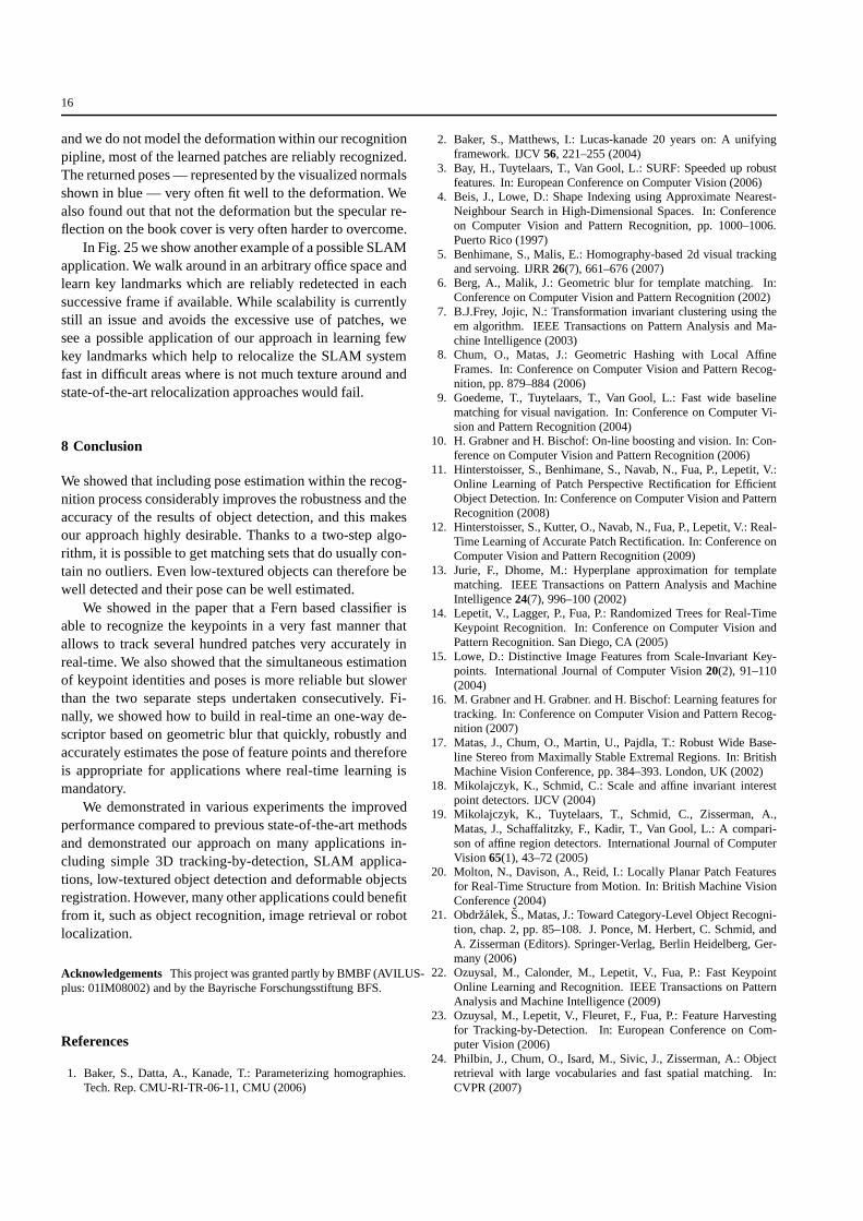
In Fig. 25 we show another example of a possible SLAMapplication. We walk around in an arbitrary office space andlearn key landmarks which are reliably redetected in eachsuccessive frame if available. While scalability is currentlystill an issue and avoids the excessive use of patches, wesee a possible application of our approach in learning fewkey landmarks which help to relocalize the SLAM systemfast in difficult areas where is not much texture around andstate-of-the-art relocalization approaches would fail.

8 Conclusion

We showed that including pose estimation within the recog-nition process considerably improves the robustness and theaccuracy of the results of object detection, and this makesour approach highly desirable. Thanks to a two-step algo-rithm, it is possible to get matching sets that do usually con-tain no outliers. Even low-textured objects can therefore bewell detected and their pose can be well estimated.

We showed in the paper that a Fern based classifier isable to recognize the keypoints in a very fast manner thatallows to track several hundred patches very accurately inreal-time. We also showed that the simultaneous estimationof keypoint identities and poses is more reliable but slowerthan the two separate steps undertaken consecutively. Fi-nally, we showed how to build in real-time an one-way de-scriptor based on geometric blur that quickly, robustly andaccurately estimates the pose of feature points and thereforeis appropriate for applications where real-time learning ismandatory.

We demonstrated in various experiments the improvedperformance compared to previous state-of-the-art methodsand demonstrated our approach on many applications in-cluding simple 3D tracking-by-detection, SLAM applica-tions, low-textured object detection and deformable objectsregistration. However, many other applications could benefitfrom it, such as object recognition, image retrieval or robotlocalization.

Acknowledgements This project was granted partly by BMBF (AVILUS-plus: 01IM08002) and by the Bayrische Forschungsstiftung BFS.

References

1. Baker, S., Datta, A., Kanade, T.: Parameterizing homographies.Tech. Rep. CMU-RI-TR-06-11, CMU (2006)

2. Baker, S., Matthews, I.: Lucas-kanade 20 years on: A unifyingframework. IJCV56, 221–255 (2004)

3. Bay, H., Tuytelaars, T., Van Gool, L.: SURF: Speeded up robustfeatures. In: European Conference on Computer Vision (2006)

4. Beis, J., Lowe, D.: Shape Indexing using Approximate Nearest-Neighbour Search in High-Dimensional Spaces. In: Conferenceon Computer Vision and Pattern Recognition, pp. 1000–1006.Puerto Rico (1997)

5. Benhimane, S., Malis, E.: Homography-based 2d visual trackingand servoing. IJRR26(7), 661–676 (2007)

6. Berg, A., Malik, J.: Geometric blur for template matching. In:Conference on Computer Vision and Pattern Recognition (2002)

7. B.J.Frey, Jojic, N.: Transformation invariant clustering using theem algorithm. IEEE Transactions on Pattern Analysis and Ma-chine Intelligence (2003)

8. Chum, O., Matas, J.: Geometric Hashing with Local AffineFrames. In: Conference on Computer Vision and Pattern Recog-nition, pp. 879–884 (2006)

9. Goedeme, T., Tuytelaars, T., Van Gool, L.: Fast wide baselinematching for visual navigation. In: Conference on ComputerVi-sion and Pattern Recognition (2004)

10. H. Grabner and H. Bischof: On-line boosting and vision. In: Con-ference on Computer Vision and Pattern Recognition (2006)

11. Hinterstoisser, S., Benhimane, S., Navab, N., Fua, P., Lepetit, V.:Online Learning of Patch Perspective Rectification for EfficientObject Detection. In: Conference on Computer Vision and PatternRecognition (2008)

12. Hinterstoisser, S., Kutter, O., Navab, N., Fua, P., Lepetit, V.: Real-Time Learning of Accurate Patch Rectification. In: Conference onComputer Vision and Pattern Recognition (2009)

13. Jurie, F., Dhome, M.: Hyperplane approximation for templatematching. IEEE Transactions on Pattern Analysis and MachineIntelligence24(7), 996–100 (2002)

14. Lepetit, V., Lagger, P., Fua, P.: Randomized Trees for Real-TimeKeypoint Recognition. In: Conference on Computer Vision andPattern Recognition. San Diego, CA (2005)

15. Lowe, D.: Distinctive Image Features from Scale-Invariant Key-points. International Journal of Computer Vision20(2), 91–110(2004)

16. M. Grabner and H. Grabner. and H. Bischof: Learning features fortracking. In: Conference on Computer Vision and Pattern Recog-nition (2007)

17. Matas, J., Chum, O., Martin, U., Pajdla, T.: Robust Wide Base-line Stereo from Maximally Stable Extremal Regions. In: BritishMachine Vision Conference, pp. 384–393. London, UK (2002)

18. Mikolajczyk, K., Schmid, C.: Scale and affine invariant interestpoint detectors. IJCV (2004)

19. Mikolajczyk, K., Tuytelaars, T., Schmid, C., Zisserman, A.,Matas, J., Schaffalitzky, F., Kadir, T., Van Gool, L.: A compari-son of affine region detectors. International Journal of ComputerVision 65(1), 43–72 (2005)

20. Molton, N., Davison, A., Reid, I.: Locally Planar Patch Featuresfor Real-Time Structure from Motion. In: British Machine VisionConference (2004)

21. Obdrzalek,S., Matas, J.: Toward Category-Level Object Recogni-tion, chap. 2, pp. 85–108. J. Ponce, M. Herbert, C. Schmid, andA. Zisserman (Editors). Springer-Verlag, Berlin Heidelberg, Ger-many (2006)

22. Ozuysal, M., Calonder, M., Lepetit, V., Fua, P.: Fast KeypointOnline Learning and Recognition. IEEE Transactions on PatternAnalysis and Machine Intelligence (2009)

23. Ozuysal, M., Lepetit, V., Fleuret, F., Fua, P.: Feature Harvestingfor Tracking-by-Detection. In: European Conference on Com-puter Vision (2006)

24. Philbin, J., Chum, O., Isard, M., Sivic, J., Zisserman, A.: Objectretrieval with large vocabularies and fast spatial matching. In:CVPR (2007)

17

(a) (b) (c) (d)Fig. 18 Robustness of ALGO1 to deformation and occlusion.(a) Patches detected on the book in a frontal view.(b) Most of these patches aredetected even under a strong deformation.(c) The book is half occluded but some patches can still be extracted.(d) The book is almost completelyhidden but one patch is still correctly extracted. No outliers were produced.

(a) (b) (c) (d)Fig. 19 Accuracy of ALGO1 of the retrieved transformation. For each of these images,we draw the borders of the book estimated from a singlepatch. This is made possible by the fact we estimate a full perspective transform instead of only an affine one.

(a) (b) (c) (d)

(e) (f) (g) (h)Fig. 20 Some frames of a Tracking-by-Detection with ALGO1 sequence shot with a low-quality camera.(a)-(g) The book pose is retrieved ineach frame independently at 10fps. The yellow quadrangle isthe best patch obtained by ALGO1. The green quadrangle is the result of the ESMalgorithm [5] initialized with the pose obtained from this patch. The retrieved pose is very accurate despite drastic perspective and intensitieschanges and blur.(h) When the book is not visible, our method does not produce a false positive.

(a) (b) (c) (d)

(e) (f) (g) (h)Fig. 21 Another example of a Tracking-by-Detection sequence with ALGO1. The book pose is retrieved under(b) scale changes,(c-d) drasticperspective changes,(e) blur, (f) occlusion, and(g-h) deformations.

18

frame #0 frame #18 frame #61 frame #112



Fig. 22 Tracking an outlet with ALGO2. We can retrieve the camera trajectory through the scene despite very limited texture and large viewpointchanges. Since the patch is detected and its poses estimatedin every frame independently, the method is very robust to fast motion and occlusion.The two graphs show the retrieved trajectory.

Fig. 23 Application to tracking-by-detection of poorly textured objects under large viewing changes with ALGO2.

19

Fig. 24 Application to a deformable object with ALGO2. We can retrieve an accurate pose even under large deformations. While it is not donehere, such cues would be very useful to constrain the 3D surface estimation.

Fig. 25 Another example of SLAM re-localisation with ALGO2, using 8 different patches.

25. Rothganger, F., Lazebnik, S., Schmid, C., Ponce, J.: Object model-ing and recognition using local affine-invariant image descriptorsand multi-view spatial constraints. International Journal of Com-puter Vision66(3), 231–259 (2006)

26. Taylor, S., Drummond, T.: Multiple target localisationat over 100fps. In: BMVC (2009)

27. Triggs, B.: Detecting Keypoints with Stable Position, Orientationand Scale under Illumination Changes. In: European Conferenceon Computer Vision (2004)

28. Williams, B., Klein, G., Reid, I.: Real-time slam relocalisation. In:International Conference on Computer Vision (2007)

Documents

Learning Real-Time Perspective Patch Rectiﬁcationcampar.in.tum.de/pub/hinterstoisser2011ijcv/hinterstoisser2011ijcv.pdf · Learning Real-Time Perspective Patch Rectiﬁcation