Embed Size (px)
Citation preview

HAL Id: inria-00548669https://hal.inria.fr/inria-00548669
Submitted on 20 Dec 2010
HAL is a multi-disciplinary open accessarchive for the deposit and dissemination of sci-entific research documents, whether they are pub-lished or not. The documents may come fromteaching and research institutions in France orabroad, or from public or private research centers.
L’archive ouverte pluridisciplinaire HAL, estdestinée au dépôt et à la diffusion de documentsscientifiques de niveau recherche, publiés ou non,émanant des établissements d’enseignement et derecherche français ou étrangers, des laboratoirespublics ou privés.
Learning Object Representations for Visual Object ClassRecognition
Marcin Marszalek, Cordelia Schmid, Hedi Harzallah, Joost van de Weijer
To cite this version:Marcin Marszalek, Cordelia Schmid, Hedi Harzallah, Joost van de Weijer. Learning Object Represen-tations for Visual Object Class Recognition. Visual Recognition Challange workshop, in conjunctionwith ICCV, Oct 2007, Rio de Janeiro, Brazil. 2007. �inria-00548669�

Introduction Method description Experiments Summary
Learning Representations forVisual Object Class Recognition
Marcin Marszałek Cordelia SchmidHedi Harzallah Joost van de Weijer
LEAR, INRIA Grenoble, Rhône-Alpes, France
October 15th, 2007
Learning Representations for Visual Object Class Recognition M. Marszałek, C. Schmid

Introduction Method description Experiments Summary
Bag-of-FeaturesZhang, Marszałek, Lazebnik and Schmid [IJCV’07]
Bag-of-Features (BoF) is an orderless distribution of localimage features sampled from an imageThe representations are compared using χ2 distance
Channels can be combined to improve the accuracyClassification with non-linear Support Vector Machines
Learning Representations for Visual Object Class Recognition M. Marszałek, C. Schmid
Introduction Method description Experiments Summary
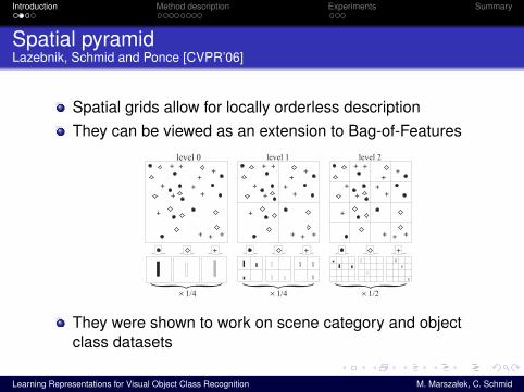
Spatial pyramidLazebnik, Schmid and Ponce [CVPR’06]
Spatial grids allow for locally orderless descriptionThey can be viewed as an extension to Bag-of-Features
get the following definition of a pyramid match kernel:
κL(X,Y ) = IL +L−1∑
�=0
12L−�
(I� − I�+1
)(2)
=12LI0 +
L∑
�=1
12L−�+1
I� . (3)
Both the histogram intersection and the pyramid match ker-nel are Mercer kernels [7].
3.2. Spatial Matching Scheme
As introduced in [7], a pyramid match kernel workswith an orderless image representation. It allows for pre-cise matching of two collections of features in a high-dimensional appearance space, but discards all spatial in-formation. This paper advocates an “orthogonal” approach:perform pyramid matching in the two-dimensional imagespace, and use traditional clustering techniques in featurespace.1 Specifically, we quantize all feature vectors into Mdiscrete types, and make the simplifying assumption thatonly features of the same type can be matched to one an-other. Each channel m gives us two sets of two-dimensionalvectors, Xm and Ym, representing the coordinates of fea-tures of type m found in the respective images. The finalkernel is then the sum of the separate channel kernels:
KL(X,Y ) =M∑
m=1
κL(Xm, Ym) . (4)
This approach has the advantage of maintaining continuitywith the popular “visual vocabulary” paradigm — in fact, itreduces to a standard bag of features when L = 0.
Because the pyramid match kernel (3) is simply aweighted sum of histogram intersections, and becausec min(a, b) = min(ca, cb) for positive numbers, we canimplement KL as a single histogram intersection of “long”vectors formed by concatenating the appropriately weightedhistograms of all channels at all resolutions (Fig. 1). ForL levels and M channels, the resulting vector has dimen-sionality M
∑L�=0 4� = M 1
3 (4L+1 − 1). Several experi-ments reported in Section 5 use the settings of M = 400and L = 3, resulting in 34000-dimensional histogram in-tersections. However, these operations are efficient becausethe histogram vectors are extremely sparse (in fact, just asin [7], the computational complexity of the kernel is linearin the number of features). It must also be noted that we didnot observe any significant increase in performance beyondM = 200 and L = 2, where the concatenated histogramsare only 4200-dimensional.
1In principle, it is possible to integrate geometric information directlyinto the original pyramid matching framework by treating image coordi-nates as two extra dimensions in the feature space.
+
+
++
+
+
++
+
+
+
++
+
++
+
+
++
+
+
+
++
+
++
+
+
++
+
+
+
+
level 2level 1level 0
� 1/4 � 1/4 � 1/2
++ +
Figure 1. Toy example of constructing a three-level pyramid. Theimage has three feature types, indicated by circles, diamonds, andcrosses. At the top, we subdivide the image at three different lev-els of resolution. Next, for each level of resolution and each chan-nel, we count the features that fall in each spatial bin. Finally, weweight each spatial histogram according to eq. (3).
The final implementation issue is that of normalization.For maximum computational efficiency, we normalize allhistograms by the total weight of all features in the image,in effect forcing the total number of features in all images tobe the same. Because we use a dense feature representation(see Section 4), and thus do not need to worry about spuri-ous feature detections resulting from clutter, this practice issufficient to deal with the effects of variable image size.
4. Feature Extraction
This section briefly describes the two kinds of featuresused in the experiments of Section 5. First, we have so-called “weak features,” which are oriented edge points, i.e.,points whose gradient magnitude in a given direction ex-ceeds a minimum threshold. We extract edge points at twoscales and eight orientations, for a total of M = 16 chan-nels. We designed these features to obtain a representationsimilar to the “gist” [21] or to a global SIFT descriptor [12]of the image.
For better discriminative power, we also utilize higher-dimensional “strong features,” which are SIFT descriptorsof 16× 16 pixel patches computed over a grid with spacingof 8 pixels. Our decision to use a dense regular grid in-stead of interest points was based on the comparative evalu-ation of Fei-Fei and Perona [4], who have shown that densefeatures work better for scene classification. Intuitively, adense image description is necessary to capture uniform re-gions such as sky, calm water, or road surface (to deal withlow-contrast regions, we skip the usual SIFT normalizationprocedure when the overall gradient magnitude of the patchis too weak). We perform k-means clustering of a randomsubset of patches from the training set to form a visual vo-cabulary. Typical vocabulary sizes for our experiments areM = 200 and M = 400.
They were shown to work on scene category and objectclass datasets
Learning Representations for Visual Object Class Recognition M. Marszałek, C. Schmid
Introduction Method description Experiments Summary
Combining kernelsBosch, Zisserman and Munoz [CIVR’07], Varma and Ray [ICCV’07]
It was shown that linear kernel combinations can belearned
Through extensive search [Bosch’07]By extending the C-SVM objective function [Varma’07]
We learn linear distance combinations insteadOur approach can still be viewed as learning a kernelWe exploit the kernel trick (it’s more than linear combinationof kernels)No kernel parameters are set by hand, everything is learnedOptimization task is more difficult
Learning Representations for Visual Object Class Recognition M. Marszałek, C. Schmid

Introduction Method description Experiments Summary
Our approach: large number of channels
In our approach images are represented with severalBoFs, where each BoF is assigned to a cell of a spatial gridWe combine various methods for sampling the image,describing the local content and organizing BoFs spatiallyWith few samplers, descriptors and spatial grids we cangenerate tens of possible representations that we call“channels”Useful channels can be found on per-class basis byrunning a multi-goal genetic algorithm
Learning Representations for Visual Object Class Recognition M. Marszałek, C. Schmid

Introduction Method description Experiments Summary
Overview of the processing chain
Image is sampledRegions are locally described with feature vectorsFeatures are quantized (assigned to a vocabulary word)and spatially ordered (assigned to a grid cell)Various channels are combined in the kernelImage is classified with an SVM
Learning Representations for Visual Object Class Recognition M. Marszałek, C. Schmid
Image→ Sampler × Local descriptor × Spatial grid⇒ Fusion→ Classification

Introduction Method description Experiments Summary
PASCAL VOC 2007 challenge
bottle car chair dog plant train
Learning Representations for Visual Object Class Recognition M. Marszałek, C. Schmid
Image→ Sampler × Local descriptor × Spatial grid⇒ Fusion→ Classification
Introduction Method description Experiments Summary
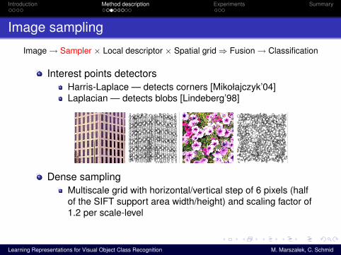
Image sampling
Interest points detectorsHarris-Laplace — detects corners [Mikołajczyk’04]Laplacian — detects blobs [Lindeberg’98]
Dense samplingMultiscale grid with horizontal/vertical step of 6 pixels (halfof the SIFT support area width/height) and scaling factor of1.2 per scale-level
Learning Representations for Visual Object Class Recognition M. Marszałek, C. Schmid
Image→ Sampler × Local descriptor × Spatial grid⇒ Fusion→ Classification

Introduction Method description Experiments Summary
Local description
SIFT — gradient orientation histogram [Lowe’04]SIFT+hue — SIFT with color [van de Weijer’06]
satura
tion
hue
hue circle
SIFT descriptor
orientation
grad
ient
hue
color descriptor
satu
ratio
n
PAS — edgel histogram [Ferrari’06]
Learning Representations for Visual Object Class Recognition M. Marszałek, C. Schmid
Image→ Sampler × Local descriptor × Spatial grid⇒ Fusion→ Classification
Introduction Method description Experiments Summary
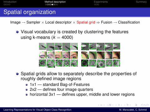
Spatial organization
Visual vocabulary is created by clustering the featuresusing k-means (k = 4000)
Spatial grids allow to separately describe the properties ofroughly defined image regions
1x1 — standard Bag-of-Features2x2 — defines four image quartershorizontal 3x1 — defines upper, middle and lower regions
Learning Representations for Visual Object Class Recognition M. Marszałek, C. Schmid
Image→ Sampler × Local descriptor × Spatial grid⇒ Fusion→ Classification

Introduction Method description Experiments Summary
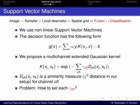
Support Vector Machines
We use non-linear Support Vector MachinesThe decision function has the following form
g(x) =∑
iαiyiK (x i , x)− b
We propose a multichannel extended Gaussian kernel
K (xj , xk ) = exp(−∑
ch
γchDch(xj , xk ))
Dch(xj , xk ) is a similarity measure (χ2 distance in oursetup) for channel ch
Problem: How to set each γch?
Learning Representations for Visual Object Class Recognition M. Marszałek, C. Schmid
Image→ Sampler × Local descriptor × Spatial grid⇒ Fusion→ Classification
Introduction Method description Experiments Summary
Support Vector Machines
We use non-linear Support Vector MachinesThe decision function has the following form
g(x) =∑
iαiyiK (x i , x)− b
We propose a multichannel extended Gaussian kernel
K (xj , xk ) = exp(−∑
ch
γchDch(xj , xk ))
Dch(xj , xk ) is a similarity measure (χ2 distance in oursetup) for channel chProblem: How to set each γch?
Learning Representations for Visual Object Class Recognition M. Marszałek, C. Schmid
Image→ Sampler × Local descriptor × Spatial grid⇒ Fusion→ Classification

Introduction Method description Experiments Summary
Weighting the channels
If we set γch to 1/Dch we almost obtain (up to channelsnormalization) the method of Zhang et al.
This approach demonstrated remarkable performance inboth VOC’05 and VOC’06We submit this approach as the “flat” method
As γch controls the weight of channel ch in the sum, it can beused to select the most useful channels
We run a genetic algorithm to optimize per-task γch,t kernelparameters and also Ct SVM parameterThe learned channel weights are used for the “genetic”submission
Learning Representations for Visual Object Class Recognition M. Marszałek, C. Schmid
Image→ Sampler × Local descriptor × Spatial grid⇒ Fusion→ Classification
Introduction Method description Experiments Summary
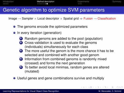
Genetic algorithm to optimize SVM parameters
The genoms encode the optimized parameters
In every iteration (generation)1 Random genoms are added to the pool (population)2 Cross-validation is used to evaluate the genoms
(individuals) simultaneously for each class3 The more useful the genom is the more chance it has to be
selected and combined with another good genom4 Information from combined genoms is randomly mixed
(crossed) and forms the next generation5 To better avoid local minimas, random genes are altered
(mutated)
Useful genes and gene combinations survive and multiply
Learning Representations for Visual Object Class Recognition M. Marszałek, C. Schmid
Image→ Sampler × Local descriptor × Spatial grid⇒ Fusion→ Classification
Introduction Method description Experiments Summary
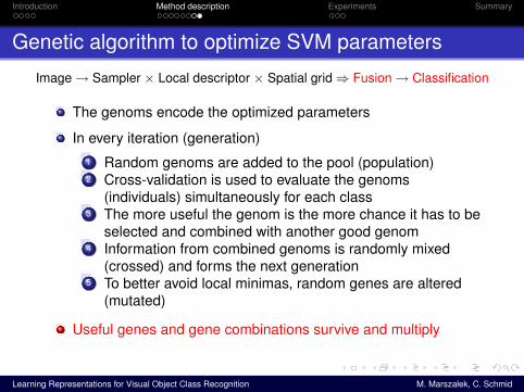
Genetic algorithm to optimize SVM parameters
The genoms encode the optimized parameters
In every iteration (generation)1 Random genoms are added to the pool (population)2 Cross-validation is used to evaluate the genoms
(individuals) simultaneously for each class3 The more useful the genom is the more chance it has to be
selected and combined with another good genom4 Information from combined genoms is randomly mixed
(crossed) and forms the next generation5 To better avoid local minimas, random genes are altered
(mutated)
Useful genes and gene combinations survive and multiply
Learning Representations for Visual Object Class Recognition M. Marszałek, C. Schmid
Image→ Sampler × Local descriptor × Spatial grid⇒ Fusion→ Classification
Introduction Method description Experiments Summary
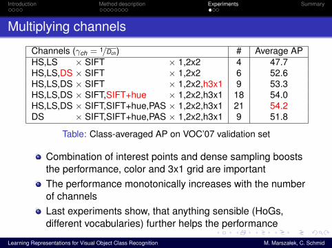
Multiplying channels
Channels (γch = 1/Dch) # Average APHS,LS × SIFT × 1,2x2 4 47.7HS,LS,DS × SIFT × 1,2x2 6 52.6HS,LS,DS × SIFT × 1,2x2,h3x1 9 53.3HS,LS,DS × SIFT,SIFT+hue × 1,2x2,h3x1 18 54.0HS,LS,DS × SIFT,SIFT+hue,PAS × 1,2x2,h3x1 21 54.2DS × SIFT,SIFT+hue,PAS × 1,2x2,h3x1 9 51.8
Table: Class-averaged AP on VOC’07 validation set
Combination of interest points and dense sampling booststhe performance, color and 3x1 grid are importantThe performance monotonically increases with the numberof channelsLast experiments show, that anything sensible (HoGs,different vocabularies) further helps the performance
Learning Representations for Visual Object Class Recognition M. Marszałek, C. Schmid
Introduction Method description Experiments Summary
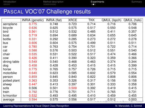
PASCAL VOC’07 Challenge resultsINRIA (genetic) INRIA (flat) XRCE TKK QMUL (lspch) QMUL (hsls)
aeroplane 0.775 0.748 0.723 0.714 0.716 0.706bicycle 0.636 0.625 0.575 0.517 0.550 0.548bird 0.561 0.512 0.532 0.485 0.411 0.357boat 0.719 0.694 0.689 0.634 0.655 0.645bottle 0.331 0.292 0.285 0.273 0.272 0.278bus 0.606 0.604 0.575 0.499 0.511 0.511car 0.780 0.763 0.754 0.701 0.722 0.714cat 0.588 0.576 0.503 0.512 0.551 0.540chair 0.535 0.531 0.522 0.517 0.474 0.466cow 0.426 0.411 0.390 0.323 0.359 0.366dining table 0.549 0.540 0.468 0.463 0.374 0.344dog 0.458 0.428 0.453 0.415 0.415 0.399horse 0.775 0.765 0.757 0.726 0.715 0.715motorbike 0.640 0.623 0.585 0.602 0.579 0.554person 0.859 0.845 0.840 0.822 0.808 0.806potted plant 0.363 0.353 0.326 0.317 0.156 0.158sheep 0.447 0.413 0.397 0.301 0.333 0.358sofa 0.506 0.501 0.509 0.392 0.419 0.415train 0.792 0.776 0.751 0.711 0.765 0.731tv/monitor 0.532 0.493 0.495 0.410 0.459 0.455average 0.594 0.575 0.556 0.517 0.512 0.503
Learning Representations for Visual Object Class Recognition M. Marszałek, C. Schmid
Introduction Method description Experiments Summary
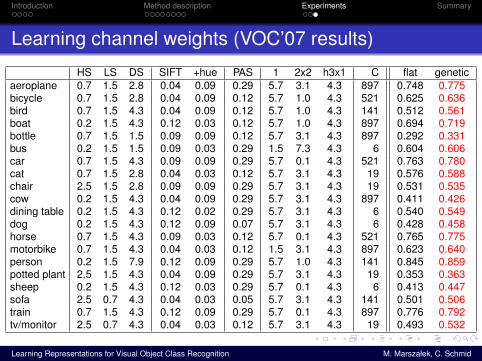
Learning channel weights (VOC’07 results)
HS LS DS SIFT +hue PAS 1 2x2 h3x1 C flat geneticaeroplane 0.7 1.5 2.8 0.04 0.09 0.29 5.7 3.1 4.3 897 0.748 0.775bicycle 0.7 1.5 2.8 0.04 0.09 0.12 5.7 1.0 4.3 521 0.625 0.636bird 0.7 1.5 4.3 0.04 0.09 0.12 5.7 1.0 4.3 141 0.512 0.561boat 0.2 1.5 4.3 0.12 0.03 0.12 5.7 1.0 4.3 897 0.694 0.719bottle 0.7 1.5 1.5 0.09 0.09 0.12 5.7 3.1 4.3 897 0.292 0.331bus 0.2 1.5 1.5 0.09 0.03 0.29 1.5 7.3 4.3 6 0.604 0.606car 0.7 1.5 4.3 0.09 0.09 0.29 5.7 0.1 4.3 521 0.763 0.780cat 0.7 1.5 2.8 0.04 0.03 0.12 5.7 3.1 4.3 19 0.576 0.588chair 2.5 1.5 2.8 0.09 0.09 0.29 5.7 3.1 4.3 19 0.531 0.535cow 0.2 1.5 4.3 0.04 0.09 0.29 5.7 3.1 4.3 897 0.411 0.426dining table 0.2 1.5 4.3 0.12 0.02 0.29 5.7 3.1 4.3 6 0.540 0.549dog 0.2 1.5 4.3 0.12 0.09 0.07 5.7 3.1 4.3 6 0.428 0.458horse 0.7 1.5 4.3 0.09 0.03 0.12 5.7 0.1 4.3 521 0.765 0.775motorbike 0.7 1.5 4.3 0.04 0.03 0.12 1.5 3.1 4.3 897 0.623 0.640person 0.2 1.5 7.9 0.12 0.09 0.29 5.7 1.0 4.3 141 0.845 0.859potted plant 2.5 1.5 4.3 0.04 0.09 0.29 5.7 3.1 4.3 19 0.353 0.363sheep 0.2 1.5 4.3 0.12 0.03 0.29 5.7 0.1 4.3 6 0.413 0.447sofa 2.5 0.7 4.3 0.04 0.03 0.05 5.7 3.1 4.3 141 0.501 0.506train 0.7 1.5 4.3 0.12 0.09 0.29 5.7 0.1 4.3 897 0.776 0.792tv/monitor 2.5 0.7 4.3 0.04 0.03 0.12 5.7 3.1 4.3 19 0.493 0.532
Learning Representations for Visual Object Class Recognition M. Marszałek, C. Schmid
Introduction Method description Experiments Summary
Summary
We have shown that using a large number of channelshelps recognition due to complementary informationWe have demonstrated how it is possible to generate tensof useful channelsWe have proposed to use a genetic algorithm to discoverthe most useful channels on per-class basisThe experimental results show excellent performance
Learning Representations for Visual Object Class Recognition M. Marszałek, C. Schmid

Introduction Method description Experiments Summary
Thank you for your attention
I will be glad to answer your questions
Learning Representations for Visual Object Class Recognition M. Marszałek, C. Schmid