Embed Size (px)
Citation preview

Learning Multi-market Microstructure from Order Book Data
Geonhwan Ju∗, Kyoung-Kuk Kim†, Dong-Young Lim‡
Korea Advanced Institute of Science and Technology
May 2019
Abstract
In this paper, we investigate market behaviors at high-frequency using neural networks
trained with order book data. Experiments are done intensively with 110 asset pairs covering
97% of spot-futures pairs in the Korea Exchange. An efficient training scheme that improves
the performance and training stability is suggested, and using the proposed scheme, the lead-lag
relationship between spot and futures markets are measured by comparing the performance gains
of each market data for predicting the other. In addition, the gradients of the trained model
are analyzed to understand some important market features that neural networks learn through
training, revealing characteristics of the market microstructure. Our results show that highly
complex neural network models can successfully learn market features such as order imbalance,
spread-volatility correlation, and mean reversion.
Keywords: high-frequency data; limit order book; neural network; lead-lag relationship; mar-
ket microstructure
1 Introduction
The wide adoption and large market share of high-frequency trading and algorithmic trading is no
news in the current financial markets. This practice also called quantitative trading in the financial
markets has been brought by three major components: first, the availability of huge and detailed
∗Corresponding author, Industrial and Systems Engineering, E-mail: [email protected]†Industrial and Systems Engineering, E-mail: [email protected]‡Industrial and Systems Engineering, E-mail: [email protected]
1

trading data from financial markets, second, advances in computing power and storage capability,
and third, significant developments in trading algorithms. Based on SEC’s concept release on
the equity market structure, high-frequency trading is responsible for 50% or higher of trading
volumes in the US equity markets. Such a substantial proportion of high-frequency trading brings
the demand for revisiting some stylized facts derived from low frequency data, and analyzing the
nature of the market structure with a view of high-frequency dynamics. The main content of this
paper is to accomplish this task using neural networks which are trained to predict short-term price
movements with order book data, particularly because neural networks are known to perform well
for large and complex datasets.
A great deal of effort to predict stock prices has already been devoted by academic researchers
and practitioners. There are many works which employed both support vector machine (SVM)
or artificial neural network (ANN) to develop a prediction system. We refer the reader to recent
survey papers rather than enumerating all related studies. Sapankevych and Sankar [2009] provided
a good survey of the SVM approach in financial market prediction and many applications for time
series data. Li and Ma [2010] surveyed the application of ANNs in forecasting asset prices. After
entering the high-frequency world, the form of data has changed from daily time series data to
huge and high dimensional TAQ historical data. Thus, ANN armed with a deep neural network
that can accommodate ‘big data’ has become more preferable in predicting future price movements.
Except for Kercheval and Zhang [2015] who use SVMs, neural network models, mainly recurrent
neural network (RNN), are considered to learn future price movements from limit order books, as
in Dixon [2017], Sirignano [2017] and Sirignano and Cont [2018].
In this paper, we suggest an efficient network architecture and training schemes to improve the
performance and training stability, which ensures the capability of the network to learn various
market features from raw data. The performance of two popular neural network architectures,
multi-layer perceptron (MLP) and RNN, are compared and the results indicate that MLP outper-
forms RNN in terms of prediction power across a wide range of assets if various input features are
preprocessed and fed into the network. After verifying the training stability and the performance
of the network, we measure the lead-lag relationship between the futures market and the spot mar-
ket of the underlying at a high-frequency level, and identify market features that drive the price
dynamics.
To investigate the lead-lag relationship in futures and spot markets with a tick-level data, we
define and compute a performance gain, a measure about how informative each market data is to
forecast price movements of the other market. When futures market data are used as additional
input data for predicting the next spot price movements, there is a substantial increase in perfor-
mance compared to the model solely trained with the spot market data. On the other hand, it turns
2

out that stock market data is obsolete for looking ahead futures prices. This shows the existence of
information asymmetry between the futures and spot markets. This finding is consistent with the
majority of results in the literature. See Kawaller et al. [1987], Stoll and Whaley [1990], Abhyankar
[1999], Min and Najand [1999], Judge and Reancharoen [2014] and references therein. Furthermore,
we find that such lead-lag relationships are observed regardless of trading activity level.
A gradient-based analysis method is proposed to interpret the market features that network
learned from market data. Many previous works focused on modeling the market dynamics with
selected features such as bid/ask imbalance or order flows to analyze micro-movements (Cao et al.
[2009], Gould and Bonart [2016], Yang and Zhu [2016], and Cont et al. [2014]). However, in terms of
predictive power, recent approaches with machine learning techniques show better performance as in
Kercheval and Zhang [2015], Dixon [2017], and Sirignano and Cont [2018]. Machine learning models
can handle high-dimensional features such as the full state of a limit order book. But one caveat is
that little analysis has been done to interpret the trained market behaviors of prediction models.
From the gradient of each input feature set, it is verified that models successfully learn peculiar
market behaviors such as order imbalance, spread-volatility correlation, and mean reversion.
The rest of the paper is organized as follows. Section 2 describes the market data and experi-
mental environments and introduces basic network architectures. An efficient network architecture
and training scheme is proposed in Section 3. Finally, Section 4 reports the results of analyses on
the lead-lag relationship and market microstructure.
2 Preliminaries
Let us first describe our dataset from the Korean stock/futures markets, and how input features
are preprocessed from raw data in detail. Next, the basic architectures of MLP and RNN are
introduced. Experimental environments including hyper-parameters, frameworks, and hardware
are also reported at the end of this section.
2.1 Data and Market Features
This study uses the entire intra-day limit orders and transactions data from the Korea Exchange,
covering one month from 15 Nov to 13 Dec 2017. These records were obtained during continuous
normal trading hours, from 9:00 a.m. to 3:30 p.m. for 19 business days during the period. The
dataset consists of 110 stocks and their nearby-maturity futures, representing about 97% of total
pairs (110 out of 113) listed in the Korea Exchange. More specifically, the dataset includes
3

• tickers of the assets traded;
• submission, cancellation, and amendment of the limit orders and their time stamps;
• transaction time, price, quantity, and type (buy or sell).
From these records, we construct a basic limit order book (LOB) feature set:{pa,it , pb,it , v
a,it , vb,it
}10
i=1
where pa,it is the ask price of the ith level at time t, and va,it represents the volume of the correspond-
ing ask level of limit order book. Prices and volumes of bid orders are pb,it and vb,it , respectively.
For smaller i, the price is closer to the mid-price. Features include ticks with 0 volume to maintain
the tick difference between levels consistent. By convention, the best bid/ask price is considered as
the first level, i.e., i = 1.
Labels are calculated based on whether the target price will increase, stay or decrease over a
small time interval ∆t. The target price is the best bid/ask price in the futures/stock markets, and
∆t is defined as a fixed time interval: {0.2s, 0.5s, 1s, 2s, 3s, 4s, 5s} where the time unit s is second.
In addition to the basic LOB features, we describe additional input features to improve the
performance of the proposed model. This work is motivated by the path-dependency of price
processes. Although most mathematical models for high-frequency trading assume that the price
evolution follows a Markov process for analytical tractability, indeed, many empirical studies find
evidence on the non-Markovian nature of price changes. See Cartea et al. [2015] and Sirignano
and Cont [2018]. Contrary to RNNs which is capable of analyzing sequential data by the network
architecture, the activations in MLPs flow only from the input layer to the output layer. Thus,
we need to manually supply historical information as inputs for MLPs to reach satisfactory results
when the labels heavily rely on historical data. We use three different path dependent features:
moving average prices, order flows, and arrival rates. By conducting comprehensive experiments,
we find that the inclusion of such path dependent features is critical in improving the performance
of MLPs.
We use seven different time windows {5s, 10s, 60s, 120s, 180, 240s, 300s} for each time-sensitive
feature, meaning that we calculate the values of each input feature by looking at the data between
t−u and t where u = 5s, 10s, etc and t is the current time. The first time-sensitive quantity, moving
average price is one of the most popular and simplest technical indicators to identify trends, and
it is calculated by averaging the volume weighted average prices (VWAP). More specifically, there
are two types of VWAP:
pa,1t va,1t + pb,1t vb,1t
va,1t + vb,1t
,pa,1t vb,1t + pb,1t va,1t
va,1t + vb,1t
4

where the latter of the two values is referred to as smart price in Kearns and Nevmyvaka [2013].
The second time-sensitive feature is the order flow which is defined as the net difference of limit
order volume changes at each price level during a fixed time window. Order flows with varying
time windows at each of the price levels show how market participants’ overall demand and supply
change over time. Lastly, we introduce the arrival rate of all limit orders over a fixed window, to
capture the two well known intra-day trading patterns. When we plot transaction volumes with
respect to the time of the day, it is typically U-shaped because trading is relatively more active
at the beginning and at the end of the day. Notably, one can observe that transactions driven by
market orders cluster together, which is the so-called volume clustering. These phenomena are well
demonstrated in Cartea et al. [2015]. Arrival rates enable models to determine whether the current
market state is active or calm.
2.2 Network Architecture and Experimental Design
Multi-layer Perceptron. An MLP is a basic form of feedforward neural networks, composed
of one input layer, hidden layers, and one output layer. Let X = (x1 x2 · · · xm) be an input
vector and output Y where m is the number of input features. For price movements, there are
three possible outcomes, down, stay and up, and the probability for each direction is calculated by
applying a softmax function to the 3 output variables, which are called logits.
Figure 1: Architecture of an MLP.
Consider a two-layer feed forward network with k nodes per layer as shown in Figure 1. The
input value for each node is computed by a weighted sum of the values for the previous nodes plus
5

Table 1: Configuration of an MLP model.1
number of hidden layers 2
number of nodes per hidden layer 1000
loss function negative log likelihood (NLL)
activation function ReLU
normalization batch normalization
optimizer stochastic gradient descent (SGD)
a bias term: in matrix form,
H(1) =(h(1)1 h
(1)2 · · · h(1)k
)= f
(XW (1) + b(1)
),
where W (1) =(w
(1)ij
){1≤i≤m,1≤j≤k}
is the weight matrix, b(1) = (b(1)1 b
(1)2 · · · b(1)k ) is the bias
vector and f is the activation function. Similarly, we can compute H(2) = f(H(1)W (2) + b(2)
).
Then, the output layer generates three output logits yi, which are sent to a softmax function to
obtain probabilities for each direction. We denote the final output Y = softmax ((y1 y2 y3)) =
softmax(H(2)W (3) + b(3)
).
The goal of training the MLP model is to properly adjust the network parameters Θ =(W (1),W (2),W (3), b(1), b(2), b(3)
)so that some suitable loss function L(Y, Y ) is minimized. The
most common approaches to minimize the loss function are stochastic gradient descent algorithms.
Remark 1 When two or more hidden layers are used, we call it a deep neural network. As
the number of hidden layers grows, the model becomes more capable of learning a very complex
function. However, we might encounter tricky problems such as overfitting or vanishing gradient
which extremely slows down the training. Several techniques have been proposed to alleviate these
problems in many aspects. Glorot and Bengio [2010] found that a significant improvement can
be achieved by replacing the sigmoid function, σ(x) = 1/(1 + e−x), with ReLU (Rectified Linear
Unit) function, ReLU(x) = max(x, 0), as an activation function. Ioffe and Szegedy [2015] suggested
‘batch normalization’ whose function is two-fold. First, it normalizes scales and second, it shifts
the output just before the activation function of each hidden layer, allowing each layer to learn
more independently by reducing covariate shift. Table 1 summarizes the network architecture of
our model.
1We searched the optimal architecture without overfitting or underfitting through experiments. The search range
is [1,10] for the number of hidden layers, and [100,2000] for the number of hidden nodes per layer.
6
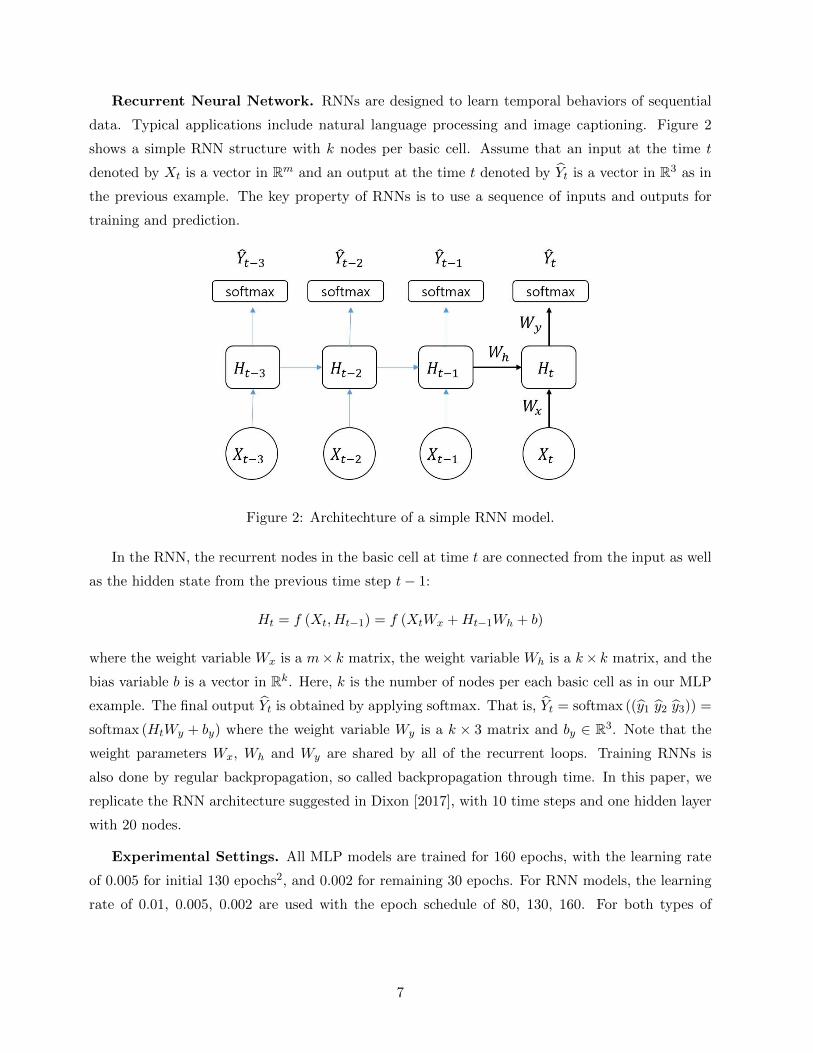
Recurrent Neural Network. RNNs are designed to learn temporal behaviors of sequential
data. Typical applications include natural language processing and image captioning. Figure 2
shows a simple RNN structure with k nodes per basic cell. Assume that an input at the time t
denoted by Xt is a vector in Rm and an output at the time t denoted by Yt is a vector in R3 as in
the previous example. The key property of RNNs is to use a sequence of inputs and outputs for
training and prediction.
Figure 2: Architechture of a simple RNN model.
In the RNN, the recurrent nodes in the basic cell at time t are connected from the input as well
as the hidden state from the previous time step t− 1:
Ht = f (Xt, Ht−1) = f (XtWx +Ht−1Wh + b)
where the weight variable Wx is a m× k matrix, the weight variable Wh is a k× k matrix, and the
bias variable b is a vector in Rk. Here, k is the number of nodes per each basic cell as in our MLP
example. The final output Yt is obtained by applying softmax. That is, Yt = softmax ((y1 y2 y3)) =
softmax (HtWy + by) where the weight variable Wy is a k × 3 matrix and by ∈ R3. Note that the
weight parameters Wx, Wh and Wy are shared by all of the recurrent loops. Training RNNs is
also done by regular backpropagation, so called backpropagation through time. In this paper, we
replicate the RNN architecture suggested in Dixon [2017], with 10 time steps and one hidden layer
with 20 nodes.
Experimental Settings. All MLP models are trained for 160 epochs, with the learning rate
of 0.005 for initial 130 epochs2, and 0.002 for remaining 30 epochs. For RNN models, the learning
rate of 0.01, 0.005, 0.002 are used with the epoch schedule of 80, 130, 160. For both types of
7

networks, we use the batch size of 3,000, `2 regularization parameter of 0.01, and the stochastic
gradient descent (SGD) optimizer with momentum of 0.9.
The whole dataset is split into two, 15 days of the training set and four days of the test set,
and all of the experiments are done with seven-fold cross-validation by changing training and test
sets.3To address the label imbalance issue, the loss contribution of each label is set to be proportional
to the inverse of the ratio of the label. To be specific, this label ratios are the ratios of the number
of down, stay, or up labels to the number of samples. We use PyTorch 0.3, and all models are
trained on a DGX-1 server with Dual Xeon E5-2698 and eight Tesla V100 GPUs.
Each training took 10 minutes on average using a single GPU, resulting in the total computation
time of 130 hours for all 110 assets with seven-fold cross-validation. The performance of the model
is measured by the area under the receiver operating characteristic (ROC) curve or simply the area
under the curve (AUC). Since AUC is a measure for binary classification, one-versus-all AUC scores
of three directions (down, stay, up) are averaged to get the final score.
3 Experiments for the Network Design
Several experiments are done to determine the architecture and the training scheme in order to im-
prove performance and stability. First, we introduce the multi-task training scheme that effectively
prevents overfitting while providing predictions for multiple time windows at the same time, with
little additional computational cost. We also compare two architectures, MLP and RNN. Although
RNN is a common approach for learning sequential features, we show that MLP is simple and
effective in terms of prediction power when various preprocessed features are fed together.
3.1 Multi-Task Training
One of the most common problems with training from the imbalanced dataset is overfitting, the
loss of generalization power due to fitting training data too closely. Overfitting easily occurs when
the label imbalance is severe while the model capacity is high. Figure 3 shows the typical training
curve of an overfitted model. While training loss continuously decreases toward 0, test loss starts
to increase after a certain point. Such occurrence of overfitting can be measured by comparing the
2Since the number of data varies with asset, longer training epochs are required for assets with less market activity.
We find that 160 epochs are enough to guarantee the convergence for all assets.3From the cross-validation results, we found that using training data whose dates are after the test set gives no
performance gain on predicting the micro-movements. This is mainly due to the highly localized characteristics of
the short-term price dynamics.
8
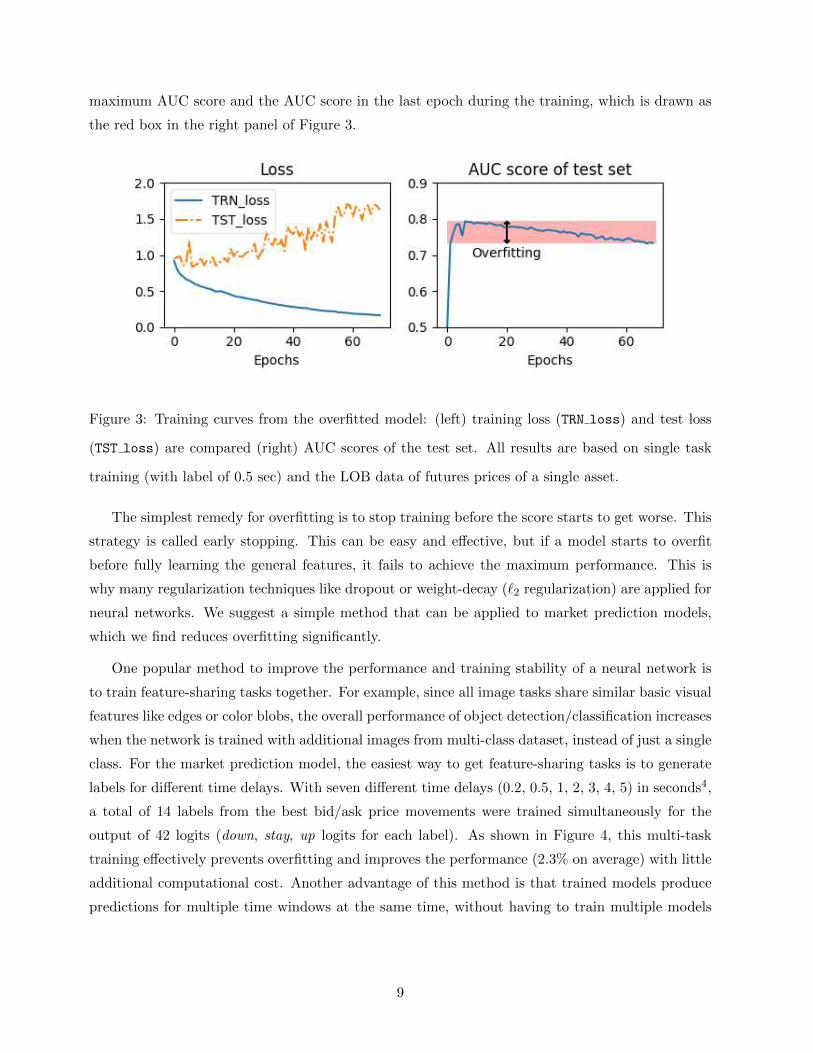
maximum AUC score and the AUC score in the last epoch during the training, which is drawn as
the red box in the right panel of Figure 3.
Figure 3: Training curves from the overfitted model: (left) training loss (TRN loss) and test loss
(TST loss) are compared (right) AUC scores of the test set. All results are based on single task
training (with label of 0.5 sec) and the LOB data of futures prices of a single asset.
The simplest remedy for overfitting is to stop training before the score starts to get worse. This
strategy is called early stopping. This can be easy and effective, but if a model starts to overfit
before fully learning the general features, it fails to achieve the maximum performance. This is
why many regularization techniques like dropout or weight-decay (`2 regularization) are applied for
neural networks. We suggest a simple method that can be applied to market prediction models,
which we find reduces overfitting significantly.
One popular method to improve the performance and training stability of a neural network is
to train feature-sharing tasks together. For example, since all image tasks share similar basic visual
features like edges or color blobs, the overall performance of object detection/classification increases
when the network is trained with additional images from multi-class dataset, instead of just a single
class. For the market prediction model, the easiest way to get feature-sharing tasks is to generate
labels for different time delays. With seven different time delays (0.2, 0.5, 1, 2, 3, 4, 5) in seconds4,
a total of 14 labels from the best bid/ask price movements were trained simultaneously for the
output of 42 logits (down, stay, up logits for each label). As shown in Figure 4, this multi-task
training effectively prevents overfitting and improves the performance (2.3% on average) with little
additional computational cost. Another advantage of this method is that trained models produce
predictions for multiple time windows at the same time, without having to train multiple models
9

separately for different labels. Figure 5 is the histogram of the difference between training loss and
test loss, which is another popular overfitting measure.
Figure 4: Overfitting measures from single task training and multi-task training. Histograms are
based on overfitting measures of all the futures prices of 110 assets.
Figure 5: Difference between training and test loss for single task training and multi-task training.
4We tried longer time delays up to 60 seconds, and 7 labels were enough to improve the training stability. Since
labels with longer time delay are less correlated with short-term price movements, using more labels with longer time
delays results in underfitting.
10
3.2 MLP vs. RNN
RNNs are designed to process sequential data effectively. They are widely used for many practical
tasks such as speech recognition and machine translation. Market data is obviously sequential.
Thus, Dixon [2017] and Sirignano and Cont [2018] trained RNNs for market data prediction mainly
with LOB states, expecting the networks to learn time-sensitive features of the market without any
preprocessing.
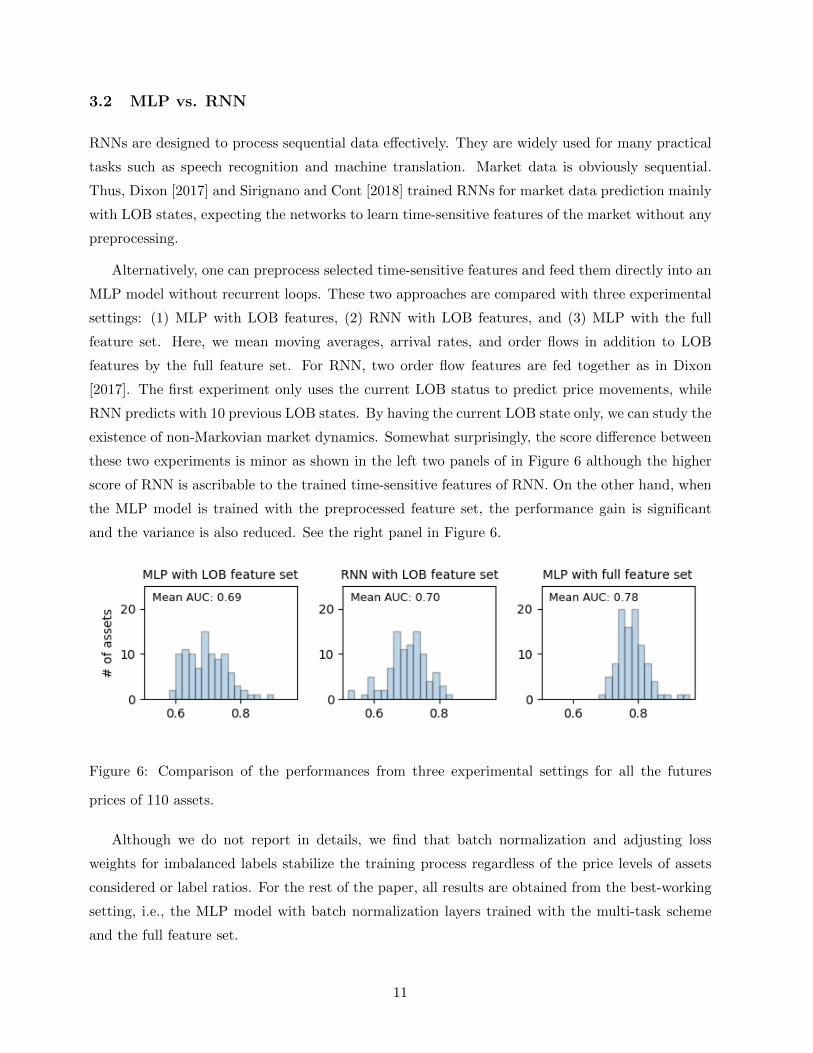
Alternatively, one can preprocess selected time-sensitive features and feed them directly into an
MLP model without recurrent loops. These two approaches are compared with three experimental
settings: (1) MLP with LOB features, (2) RNN with LOB features, and (3) MLP with the full
feature set. Here, we mean moving averages, arrival rates, and order flows in addition to LOB
features by the full feature set. For RNN, two order flow features are fed together as in Dixon
[2017]. The first experiment only uses the current LOB status to predict price movements, while
RNN predicts with 10 previous LOB states. By having the current LOB state only, we can study the
existence of non-Markovian market dynamics. Somewhat surprisingly, the score difference between
these two experiments is minor as shown in the left two panels of in Figure 6 although the higher
score of RNN is ascribable to the trained time-sensitive features of RNN. On the other hand, when
the MLP model is trained with the preprocessed feature set, the performance gain is significant
and the variance is also reduced. See the right panel in Figure 6.
Figure 6: Comparison of the performances from three experimental settings for all the futures
prices of 110 assets.
Although we do not report in details, we find that batch normalization and adjusting loss
weights for imbalanced labels stabilize the training process regardless of the price levels of assets
considered or label ratios. For the rest of the paper, all results are obtained from the best-working
setting, i.e., the MLP model with batch normalization layers trained with the multi-task scheme
and the full feature set.
11
4 Market Analysis using Neural Network Models
This section provides an analysis of multi-market microstructure based on the trained neural net-
work model. Section 4.1 examines the information inefficiency between the futures market and
the spot market to investigate their lead-lag relationship. Next, Section 4.2 discusses how market
features are interrelated to the micro-movements of market prices, by analyzing the gradients with
respect to each feature set.
4.1 Multi-Market Information Inefficiency
There is a rich literature on the lead-lag relationship between the futures and spot markets.
Although reported findings are diverse in methodologies, countries, data frequency/period, the
majority of them report that there is a tendency for the futures market to lead the spot market. To
name a few, Kawaller et al. [1987] showed that S&P futures prices significantly affect subsequent
S&P 500 index movements based on a vector auto-regression model. Stoll and Whaley [1990] gave
a similar finding that S&P 500 and major market index futures tend to lead the stock market
by about five minutes on average. Then, a variety of quantitative methods have been used to
clarify the relationship between derivative markets and their underlying asset markets. We refer
the reader to Judge and Reancharoen [2014] for an overview of the literature until 2014. More
recently, Huth and Abergel [2014] studied a lead-lag relationship measured by a cross-correlation
function using tick-by-tick data. They showed that the lead-lag relationship is closely related to
the level of liquidity, observing that more liquid assets tend to lead less liquid assets. Zhou and
Wu [2016] used four different econometric models to see a high-frequency relationship between the
futures market and the spot market. In Wang et al. [2017], a thermal optimal path method is
employed to identify the long term and the short-term relationship between the two markets in
China.
Our analysis is distinguished from the literature in three ways. Firstly, on the contrary to
popular econometric models such as vector auto-regression or other linear models that focus on the
linear interdependence among multivariate time series, our method is able to capture non-linear
relationships between futures and spot price dynamics as well as their LOB states. Secondly, the
neural network model reflects short-term information inefficiency, which may dissipate in a very
short time. Numerous papers investigated the existence of the lead-lag relationship in a variety
of time scales, however, they usually focus on relatively low-frequency data so that it may be
inadequate to extend those findings to the short-run causal relationship in a high-frequency setting.
12

Table 2: Four experimental settings to obtain performance gains.
Experiment Input data Prediction
A spot spot
B futures, spot spot
C futures futures
D futures, spot futures
Lastly, our analysis covers almost every pair of futures contracts and their underlying assets in the
Korea Exchange based on our massive and complete data set, whereas results in the literature are
often based on stock index futures and underlying spot indices. This advantage enables us to look
into any relationship between information asymmetry (the futures and spot markets) and liquidity
asymmetry (various assets with different market activity levels).
In an ideal situation, the relationship between the price of a futures contract Ft and the price
of the underlying asset St at the time t is given by
Ft = Ste(r−d)(T−t) (1)
where r is the risk free interest rate, d is the dividend yield of the underlying asset and T is
the maturity of the futures contract under the assumption that r and d are known and constant.
In perfectly efficient markets, the violation of the relation (1) should disappear instantaneously.
However, if there is information inefficiency between the two markets, the lead-lag relationship
could arise. Indeed, many empirical studies reported that futures prices move first, and then pull
stock prices to remove arbitrage.
To investigate such market behaviors, we consider four experimental settings A , B, C , and
D of which details are shown in Table 2. For example, the network of Experiment A predicts
the direction of spot prices using the full feature set from the spot market only. On the other
hand, the network of Experiment B uses all the features from both markets to predict spot price
movements. Comparing the performances of A and B would reveal whether the futures market
data is informative to forecast spot price movements, and we consider this as the performance
gain from the futures market. Similarly, the performance gain from the spot market data for
predicting futures price movements is estimated by comparing Experiment C and Experiment D .
For each asset and each cross-validation set, performance gains are calculated and averaged over
cross-validations.
We carry out experiments for 110 pairs of futures contracts and their underlying assets. The
results are visualized only for the label of the best ask price after 0.5 seconds. However, we note
13

that the outcomes are consistent across all of the fourteen labels. Figure 7 plots the histograms
of performance gains from one market to predict the movement of the other. It is apparent that
the futures market data is highly effective to improve the predictability of spot price movements.
Performance gains are positive for most assets as shown in the shaded bars in the figure. On the
other hand, the performance gains from the spot market, that is, when the spot market data is
an additional input, are distributed around zero. This implies that the spot market data is not
significantly helpful for predicting futures market price movements. Such information asymmetry
between the two markets illustrates the unidirectional flow of information from the futures market
to the spot market across a wide range of asset pairs.
Figure 7: Illustration of performance gains from multi-market data.
We also explore the behavior of information gain with respect to the degree of market activity,
defined by the average LOB changes per day. Figure 8 depicts that information asymmetry between
the two markets can be observed, irrespective of the degree of market activity.
Many papers argue that the causal relationship between futures prices and spot prices is at-
tributed to high liquidity as well as low transaction cost and less restrictive regulations in the futures
market. Along this line of arguments, we examine whether the predictive performance is influenced
by liquidity asymmetry. To proxy liquidity asymmetry, we measure the relative difference of market
activities defined by
average number of LOB changes in the futures market per day
average number of LOB changes in the spot market per day.
As the value of market activity asymmetry is away from one, there is a large imbalance of liquidity
between the two markets. Figure 9 indicates that there is no significant correlation between these
quantities.
14

Figure 8: Performance gain with respect to market activity.
Figure 9: Performance gain with respect to the relative difference in market activity.
Lastly, we analyze the performance gains for different labels in order to check the persistence
of the performance gain from the futures market in predicting spot price movements. As shown in
Figure 10, it is observed that the gain from multi-market data gradually decreases as the model
predicts price movements for a longer time scale. This observation indicates that the contribution
of the information from the futures market depreciates as the label time increases. Nevertheless, we
emphasize that models trained with multi-market data still outperform models trained on a single
market, on average even when the model predicts the spot price movements after five seconds.
15
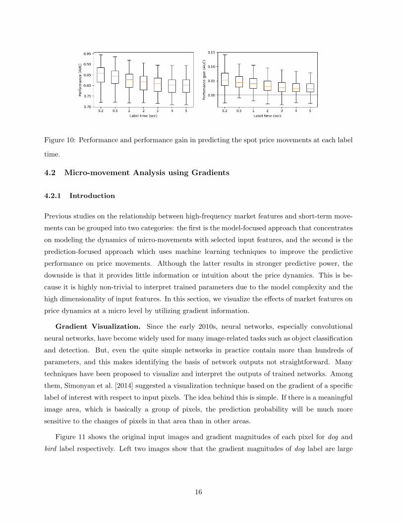
Figure 10: Performance and performance gain in predicting the spot price movements at each label
time.
4.2 Micro-movement Analysis using Gradients
4.2.1 Introduction
Previous studies on the relationship between high-frequency market features and short-term move-
ments can be grouped into two categories: the first is the model-focused approach that concentrates
on modeling the dynamics of micro-movements with selected input features, and the second is the
prediction-focused approach which uses machine learning techniques to improve the predictive
performance on price movements. Although the latter results in stronger predictive power, the
downside is that it provides little information or intuition about the price dynamics. This is be-
cause it is highly non-trivial to interpret trained parameters due to the model complexity and the
high dimensionality of input features. In this section, we visualize the effects of market features on
price dynamics at a micro level by utilizing gradient information.
Gradient Visualization. Since the early 2010s, neural networks, especially convolutional
neural networks, have become widely used for many image-related tasks such as object classification
and detection. But, even the quite simple networks in practice contain more than hundreds of
parameters, and this makes identifying the basis of network outputs not straightforward. Many
techniques have been proposed to visualize and interpret the outputs of trained networks. Among
them, Simonyan et al. [2014] suggested a visualization technique based on the gradient of a specific
label of interest with respect to input pixels. The idea behind this is simple. If there is a meaningful
image area, which is basically a group of pixels, the prediction probability will be much more
sensitive to the changes of pixels in that area than in other areas.
Figure 11 shows the original input images and gradient magnitudes of each pixel for dog and
bird label respectively. Left two images show that the gradient magnitudes of dog label are large
16

in the region where the dog presents, and the gradient map of bird label on the right highlights the
location of the bird.
Figure 11: Gradient visualization of CNN. The first and third are images from the test set of
ILSVRC-2013, and the others are images in Simonyan et al. [2014].
A similar idea can be applied to analyze the influence of input features to the output of a
network. For a neural network model G and an input vector X = (x1 x2 . . . xm), an output
Y = G(X) and gradient Gxi = ∂G(X)∂xi
are calculated via feedforward and backpropagation. A
positive Gx1 means that Y increases as x1 increases. If Gx2 is negative in addition, this implies
that the change of the output ∆Y is positively correlated to the difference of two input changes,
∆x1 −∆x2. We extend this simple relationship to multiple inputs to analyze gradient plots.
In our model, unlike images that objects can appear anywhere, the same type of information is
fed to the exact same location. This means that gradients can be averaged over the whole dataset
to observe the overall influence of each feature set on price movements. We visualize the average
gradients of outputs only for the time window of 0.5 seconds, but the patterns are similar for other
time windows as well. There are three output logits for each side of the market, so we have six
plots from down, stay, and up logits of the best ask and bid price. For the rest of this section, we
present analysis for four feature sets: LOB volume, LOB price, moving average price, and arrival
rate.
All the results reported in this section are based on the prediction results of the best bid and
ask prices in the futures markets with 110 assets utilizing the input data of the futures market.
This corresponds to Experiment C in Section 4.1.
4.2.2 Gradient Analysis of Market Features
LOB Volumes. Figure 12 shows the average gradients Gva,i , Gvb,i of six logit outputs with respect
to order volumes around the mid-price. All the gradients are averaged over 110 assets. For instance,
the top left panel is the gradient plot of the down probability of the best ask price with respect to
the volumes at ten price levels. The most prominent feature in the figure is the peak at the best
ask with positive sign and negative values at bid prices. See the dashed box in the top left panel.
17

This visualizes a well-known correlation between the bid/ask order imbalance and price movement,
as many existing studies indicate. For an illustration, assume the volume at the best ask grows
and the volume at the best bid shrinks. This order imbalance increases the down probability of
the best ask price and decreases the up probability of the best ask price, pushing the price levels
downward. Similarly, for the up or down probability of the best bid price, we see that peaks are
formed at the best bid and that bid/ask imbalance has similar effects on the target logit output.
Figure 12: Gradients of down (left), stay (middle), up (right) probabilities of the best bid/ask
prices with respect to the order volumes at ten price levels. The dashed box in the top left panel
highlights the effect of the bid/ask order imbalance on the price movement. The solid box in the
bottom right panel highlights the effect of bid order imbalance on the price movement. All gradient
plots are averaged over 110 assets.
Another interesting observation is that the effects of volumes on the bid (or ask) side on the
down/up probabilities of the best bid (or ask) are not consistent across bid (or ask) price levels.
See, for instance, the solid box in the bottom right panel. This might look counter-intuitive at
first glance because the increases in bid orders beyond the best bid seem to induce the downward
price movement. However, one can argue that this phenomenon actually indicates another order
imbalance feature, which may be called ‘bid imbalance’ or ‘ask imbalance’ depending on the type
of the order. Suppose, for a fixed total volume of orders on the bid side, bid orders become biased
toward the best bid. In other words, the orders beyond the best bid decrease while the volume
at the best bid increases. Then, the gradient plot in the solid box of Figure 12 implies that it
18
leads to an increase in the probability of the best bid to go upward. One may think of this as the
indication of the natural relationship between the market participants’ average willingness-to-buy
and the market price. To the best of the authors’ knowledge, this kind of order imbalance has not
been reported in the literature.
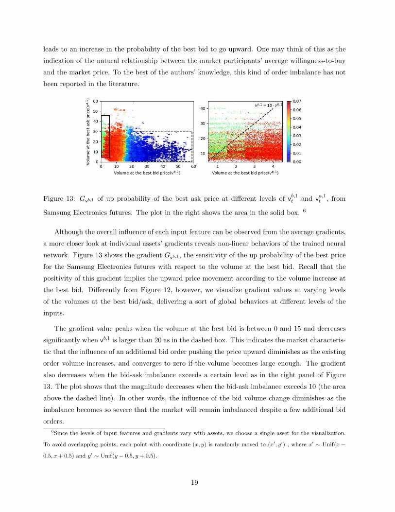
Figure 13: Gvb,1 of up probability of the best ask price at different levels of vb,1t and va,1t , from
Samsung Electronics futures. The plot in the right shows the area in the solid box. 6
Although the overall influence of each input feature can be observed from the average gradients,
a more closer look at individual assets’ gradients reveals non-linear behaviors of the trained neural
network. Figure 13 shows the gradient Gvb,1 , the sensitivity of the up probability of the best price
for the Samsung Electronics futures with respect to the volume at the best bid. Recall that the
positivity of this gradient implies the upward price movement according to the volume increase at
the best bid. Differently from Figure 12, however, we visualize gradient values at varying levels
of the volumes at the best bid/ask, delivering a sort of global behaviors at different levels of the
inputs.
The gradient value peaks when the volume at the best bid is between 0 and 15 and decreases
significantly when vb,1 is larger than 20 as in the dashed box. This indicates the market characteris-
tic that the influence of an additional bid order pushing the price upward diminishes as the existing
order volume increases, and converges to zero if the volume becomes large enough. The gradient
also decreases when the bid-ask imbalance exceeds a certain level as in the right panel of Figure
13. The plot shows that the magnitude decreases when the bid-ask imbalance exceeds 10 (the area
above the dashed line). In other words, the influence of the bid volume change diminishes as the
imbalance becomes so severe that the market will remain imbalanced despite a few additional bid
orders.
6Since the levels of input features and gradients vary with assets, we choose a single asset for the visualization.
To avoid overlapping points, each point with coordinate (x, y) is randomly moved to (x′, y′) , where x′ ∼ Unif(x −
0.5, x + 0.5) and y′ ∼ Unif(y − 0.5, y + 0.5).
19

LOB Prices. Next, we study the gradient plots of the target logit outputs with respect to the
LOB price levels. Recall that we build up the LOB feature set including ticks with 0 volume. Hence,
bid or ask prices levels are deterministic from the best bid/ask prices. Therefore, the gradients with
respect to LOB prices boil down to the gradients with respect to the overall bid/ask price levels.
This is nothing but the effect of change of variable. See Figure 14 where each gradient plot has two
values with respect to the bid price level and to the ask price level.
Figure 14: Gradients of down (left), stay (middle), up (right) probabilities of the best bid/ask
prices with respect to bid/ask price levels. All gradient plots are averaged over 110 assets.
It is notable that the signs of gradients in the left and right columns are positive with respect to
the ask price and negative with respect to the bid price while the values in the top left and bottom
right corners are relatively greater. It turns out to be illuminating if we consider those gradients
in terms of bid-ask spread and mid-price level rather than bid/ask price levels. Here, the bid-ask
spread is st = pa,1t − pb,1t and the mid-price is mt = (pa,1t + pb,1t )/2. With Y = G(X), the partial
derivatives Gst and Gmt are calculated as Gpa,1t−G
pb,1tand 2(Gpa,1t
+Gpb,1t
), respectively.
In our experiments, the average Gmt over all asset pairs is positive for down events and negative
for up events. This implies that when the mid-price level increases, the best bid/ask prices at
the next time stamp (0.5 seconds later in this set of experiments) have larger probabilities to go
down and smaller probabilities to go up. This mean reversion behavior has long been observed in
financial markets, and it is re-confirmed in our tick-level data.
20

Let us turn our attention to the gradient Gst . It is easily seen that Gst values are positive in the
left and right columns whereas they are negative in the middle column from Figure 14. This means,
first, that the widening bid-ask spread affects the down/up probabilities of the best bid and ask
prices positively, and reduces the probabilities of staying at the current price levels. In other words,
there is a higher probability of price changes at the next time stamp, which can be interpreted as
a positive correlation between tick-level price volatility and bid-ask spread. Bollerslev and Melvin
[1994] quantified this relationship with a GARCH model, and Wyart et al. [2008] modeled the
profitability of market makers, showing that adverse selection risk makes the bid-ask spread wider
when the market is volatile. Zumbach [2004] also reported a strong empirical evidence for stocks
included in FTSE 100. Secondly, the magnitudes of Gst are greater in the top left and bottom
right panels, where the target probabilities are the probabilities of the spread narrowing events.
One plausible explanation for this is that, when the bid-ask spread widens, market participants are
likely to place limit orders to fill up the order book.
Moving Average. The gradient plots for the moving average prices with varying time windows
are shown in Figure 15. For down logits, the gradient tends to decrease in the length of the time
window, and increases for up logits regardless of whether it is for the best bid or the best ask.
This observation implies that when the shorter-term moving averages increase, the best bid and
ask prices have larger probabilities of going down and smaller probabilities of going up. On the
contrary, when the longer-term moving averages increase, the best bid and ask prices have smaller
probabilities of going down and larger probabilities of going up. In both cases, the best bid and
ask prices tend to move together in a probabilistic sense. This discrepancy between short-term and
long-term moving averages indicates the existence of the price reversion to the long-term moving
average.
Arrival Rate. As shown in Figure 16, the greater arrival rate increases the probability of price
changes regardless of the time window, making bid price and ask price more volatile. Besides the
overall influence of arrival rates, arrival rates with the time windows of 60 seconds or under are
more influential than arrival rates with longer time windows. The reader is reminded that the time
delay is 0.5 seconds; however, exactly the same patterns are consistently observed for other time
delays, too. This tendency tells us that a rapid increase of arrival rates within the last one minute
induces additional volatility to the market.
To further illustrate the effects of arrival rates, we record average gradient values for the up and
down probabilities of the best bid with respect to different levels of arrival rates in Figure 17. In
other words, the figure shows a version of Figure 16 conditional on the size of an arrival rate of a
specific time window. From the two plots, we notice that the average gradient values are positive at
all levels, i.e. added volatilities due to increased order arrivals. However, their effects on up/down
21

Figure 15: Gradients of down (left), stay (middle), up (right) probabilities of the best bid/ask prices
with respect to the moving averages with varying lengths of time windows. All gradient plots are
averaged over 110 assets. Moving averages are defined as the first of the two formulas in (2.1).
probabilities diminish as arrival rates become larger. This indicates that a few extra order arrivals
affect price volatility most when the arrival rate is low compared to when order arrivals are already
quite high.
22

Figure 16: Gradients of down (left), stay (middle), up (right) probabilities of the best bid/ask
prices with respect to the arrival rates of all limit orders in varying lengths of time windows. All
gradient plots are averaged over 110 assets.
0 2 4 6 8 10 12Arrival rate
0.00
0.01
0.02
0.03
0.04
0.05
Grad
ient of u
p prob
abilit
y
0 2 4 6 8 10 12Arrival rate
0.00
0.01
0.02
0.03
0.04
0.05
Grad
ient of d
own prob
abilit
y AR_10sAR_60sAR_120sAR_300s
Figure 17: The average gradient values of up (left) and down (right) probability of the best bid
price at different levels of arrival rate, from Samsung Electronics futures.
23

5 Conclusion
This paper introduced an efficient neural network architecture and training scheme for order book
data. Multi-task training is a simple and easy way to improve the training performance and stability
with little extra cost. Preprocessing input features helped the network learn time-sensitive features.
This approach with a multi-layer perceptron model performed better compared to a recurrent neural
network model.
Using the proposed approach, the high-frequency lead-lag relationship between spot and futures
markets was examined for 110 pairs of assets. Unlike previous works that captured linear interde-
pendence, the lead-lag relationship was calculated directly by comparing the predictive power of
the neural networks with different input data. We also observed that such a lead-lag relationship
persists across different market activity levels.
Lastly, we identified the market features that drive price movements by looking into the gradients
information from trained neural networks. Many known market characteristics including bid/ask
imbalance and mean reversion are observed from gradient plots. Other market features which have
received little attention in the literature were identified as well. For instance, the order imbalances
on the bid (or ask) side have non-negligible impacts on price movements.
The findings in this work are only a small part of many possibilities that we can explore
with neural networks or we may call financial deep learning techniques. Other important market
characteristics such as order book resilience could also be explored based on similar ideas. We also
believe that the performance of prediction can be improved with larger datasets, model ensembles,
and fine-tuning. Nevertheless, a transformation of this predictive power into trading strategies in
dynamic and adaptive financial markets seems to remain as a huge challenge, in which universal
and promising outputs are yet to be seen.
Acknowledgement
The authors thank their project counterpart for providing us with valuable datasets. Constructive com-
ments from Prof. Jinwoo Shin are greatly appreciated. This work was supported by the National Research
Foundation of Korea (NRF-2019R1A2C1003144). Author names are in the alphabetical order.
References
A. Abhyankar. Linear and nonlinear granger causality: Evidence from the U.K. stock index futures
market. Journal of Futures Markets, 18:519–540, 1999.
24

T. Bollerslev and M. Melvin. Bidask spreads and volatility in the foreign exchange market: An
empirical analysis. Journal of International Economics, 36(3):355 – 372, 1994.
C. Cao, O. Hansch, , and X. Wang. The information content of an open limit-order book. Journal
of Futures Markets, 29(1):16–41, 2009.
A. Cartea, S. Jaimungal, and J. Penalva. Algorithimic and High-freqeucny Trading. Cambridge
University Press, 2015.
R. Cont, A. Kukanov, and S. Stoikov. The price impact of order book events. Journal of Financial
Econometrics, 2014.
M. Dixon. Sequence classification of the limit order book using recurrent neural networks. Journal
of Computational Science, 24:277–286, 2017.
X. Glorot and Y. Bengio. Understanding the difficulty of training deep feedforward neural ne-
towrks. Proceedings of the thirteenth international conference on artificial intelligence and statis-
tics, pages 249–256, 2010.
M.D. Gould and J. Bonart. Queue imbalance as a one-tick-ahead price predictor in a limit order
book. Market Microstructure and Liquidity, 2(2):1650006, 2016.
N. Huth and F. Abergel. High frequency lead/lag relationships - Empirical facts. Journal of
Empirical Finance, 26:41–58, 2014.
S. Ioffe and C. Szegedy. Batch normalization: Accelerating deep network training by reducing
internal covariate shift. arXiv preprint arXiv:1502.03167, 2015.
A. Judge and T. Reancharoen. An empirical examination of the lead-lag relationship between spot
and futures marekts: Evidence from Thailand. Pacific-Basic Finance Journal, 29:335–358, 2014.
I.G. Kawaller, P.D. Koch, and T.W. Koch. The temporal price relationship between S&P 500
futures and the S&P index. Journal of Finance, 42:1309–1329, 1987.
M. Kearns and Y. Nevmyvaka. Machine learning for market microstructure and high frequency
trading. In D. Easley, M. Lopez de Prado, and M. OHara, editors, High Frequency Trading -
New Realities for Traders, Markets and Regulators. Risk Books, 2013.
A. N. Kercheval and Y. Zhang. Modelling high-frequency limit order book dynamics with support
vector machines. Quantitative Finance, 15:1315–1329, 2015.
Y. Li and W. Ma. Applications of artificial neural networks in financial economics: A survey.
International Symposium on Computational Intelligence and Design, 1:211–214, 2010.
25

J. H. Min and M. Najand. A further investigation of the lead-lag relationship between the spot
market and stock index futures: Early evidence from Korea. Journal of Futures Markets, 19(2):
217–232, 1999.
N.I. Sapankevych and R. Sankar. Time series prediction using support vector machines: A survey.
IEEE Computational Intelligence Magazine, 4(2):24–38, 2009.
K. Simonyan, A. Vedaldi, and A. Zisserman. Deep inside convolutional networks: Visualising image
classification models and saliency maps. ICLR Workshop, 2014.
J. Sirignano. Deep learning for limit order books. Working paper, 2017.
J. Sirignano and R. Cont. Universal features of price formation in financial marekts: Perspectives
from deep learning. Working paper, 2018.
H.R. Stoll and R.E. Whaley. The dynamics of stock index and stock index futures returns. Journal
of Financial and Quantitative Analysis, 25, 1990.
D. Wang, J. Tu, X. Chang, and S. Li. The lead-lag relationship between the spot and futures
markets in China. Quantitative Finance, 17:1447–1456, 2017.
M. Wyart, J. Bouchaud, J. Kockelkoren, M. Potters, and M. Vettorazzo. Relation between bidask
spread, impact and volatility in order-driven markets. Quantitative Finance, 8(1):41–57, 2008.
T. Yang and L. Zhu. A reduced-form model for level-1 limit order books. Market Microstructure
and Liquidity, 2(2):1650008, 2016.
B. Zhou and C. Wu. Intraday dynamic relationships between CSI 300 index futures and spot
markets: a high-frequency analysis. Neural Computing and Applications, 27:1007–1017, 2016.
G. Zumbach. How trading activity scales with company size in the FTSE 100. Quantitative Finance,
4(4):441–456, 2004.
26