UNIVERSITY OF CALIFORNIA

Los Angeles

LEARNING, EXPERIMENTATION, AND

EQUILIBRIUM SELECTION IN GAMES

A dissertation submitted in partial satisfaction of the

requirements for the degree Doctor of Philosophy

in Economics

by

Youngse Kim

1992

c© Copyright by

Youngse Kim

1992

The dissertation of Youngse Kim is approved.

John G. Riley

Ivo Welch

David K. Levine, Committee Chair

University of California, Los Angeles

1992

ii

DEDICATION

To Hyehoon Lee, my wife and colleague economist, and Sunghwan D. Kim.

iii

Contents

1 Overview 1

2 Reputation in Participation Games 2

3 Adjustment Dynamics with Patient Players 3

4 Evolutionary Learning with Experimentations 4

5 Reference 5

iv

List of Figures

v

List of Tables

vi

ACKNOWLEDGEMENTS

I am delighted to acknowledge my thesis committee for their assistance. I wish

to thank my committee chairman, David K. Levine, for his intellectual stimulus,

valuable advice, and tireless encouragement. Joseph Ostroy and John G. Riley

have remained my mentors throughout my academic life at UCLA. Discussions

with Costas Azariadis, Sushil Bikhchandani, Kim Border, Bryan Ellickson, Drew

Fudenberg, Jack Hirshleifer, Axel Leijonhufvud, Hamid Sabourian, Lloyd Shapley,

Eric van Damme, Ivo Welch, and Bill Zame proved extremely beneficial.

I also thank Marco Celentani, In Ho Lee, and Wolfgang Pesendorfer, excellent

members of the theory student seminar group—which has been led by Professor

Levine—for intellectual and social comradery.

Financial support from the National Science Foundation, the Graduate Fel-

lowship of the University of California, and the Academic Senate of UCLA.

Finally I acknowledge my parents, my wife, and my son for their love.

vii

VITA

23 October 1962 Born, Seoul, Korea

1985 B.A., EconomicsYonsei UniversitySeoul, Korea

1987 M.A., EconomicsYonsei UniversitySeoul, Korea

March - August 1987 LecturerSchool of BusinessYonsei UniversitySeoul, Korea

1988 - 1992 Teaching Assistant and AssociateDepartment of EconomicsUniversity of CaliforniaLos Angeles, California

PUBLICATIONS AND PRESENTATIONS

Kim, Y. (October, 1990). “Characterization and Properties of ReputationEffects in Extensive Form Games.”

. (September, 1991). “Credibility, Smooth Expectations, and Infla-tion Persistence.”

. (July, 1992). “Adjustment Dynamics with Patient Players in Co-ordination Games.” UCLA Working Paper no.667.

. (October, 1992). “Adjustment, Evolution, and Equilibrium Selec-tion in Games.”

viii

ABSTRACT OF THE DISSERTATION

LEARNING, EXPERIMENTATION, AND EQUILIBRIUM

SELECTION IN GAMES

by

Youngse Kim

Doctor of Philosophy in Economics

University of California, Los Angeles, 1992

Professor David K. Levine, Chair

This dissertation addresses and resolves problem of selection among multiple

equilibria in games, by perturbing the original system and then characterizing the

outcome of resulting perturbed system.

Chapter 2 examines reputational sequential equilibrium of what we call par-

ticipation games, that have many economic applicability, such as entry deterrence

and product quality control. By perturbing the original game with types, we show

that the lower bound of the single long run player’s payoff is almost his Stack-

elberg commitment payoff in the limit as the finite horizon grows. Discontinuity

exists between the infinite horizon and the limiting finite horizon solution. Our

result is robust to a model modification in which the long run player announces

the payoff structure just before the whole game begins so that the rational type

of long run player has to mimic not only the strategy but also the initial payoff

announcement of the Stackelberg commitment type.

Chapter 3 and chapter 4 analyze a game played by randomly and anonymously

matched players from a large population. The game of interest is a multiperson

ix

coordination game with multiple strict Nash equilibria. In chapter 3, players are

fully rational, but adjustment is costly. Equilibrium outcomes are fully character-

ized as a function of group size and level of friction. We examine limiting results

and their links to static equilibrium concepts. The equivalence between risk dom-

inance and learning outcomes previously shown in two-player games fails with

three or more players. Surprisingly, the limit as the friction disappears coincides

with the selection from global perturbation and strict iterated admissibility. For

a pure coordination game, a much stronger result can be shown to support equi-

librium Pareto efficiency—as long as the friction is sufficiently small—regardless

of group size either. Finally, we also provide numerical results that have some im-

plications for several well-known experiments on coordination failure and history

dependence.

Chapter 4 clarifies the relationship between adjustment or evolutionary dy-

namics studied in the literature. Two types of dynamic process turn out to pos-

sess the power of resolving indeterminacy: the deterministic adjustment dynamics

with patient players, and the stochastic evolutionary dynamics with myopic play-

ers. Roughly speaking, the dynamically attractive outcome obtained with patient

players corresponds to the static equilibrium assuming correlated play of oppo-

nents, while the long run state obtained with noisy myopic players corresponds to

the static equilibrium selection predicted by independent play of one’s opponents.

We show that, if and only if group size equals two (ie, 2× 2 games), the dynamic

outcome from either type of process happens to coincide risk dominance. For any

pure coordination game, a much stronger result obtains supporting the Pareto

efficiency, regardless of the underlying dynamics.

x

Chapter 1

Overview

1

Chapter 2 examines reputation sequential equilibria of what we call partici-

pation games, that have many economic examples, such as entry deterrence and

product quality control. By perturbing the original game with types. we show

that the lower bound of the single long run player’s payoff is almost his Stack-

elberg commitment payoff in the limit as the finite horizon grows. Discontinuity

exists between the infinite horizon and the limiting finite horizon problem. Double

traps may exist in some important subclass of games, namely enttry- inducement

games. Our result is robust to a model modification in which the long run player

announces the payoff structure just before the whole game begins so that the ratio-

nal type of long run player has to mimic not only the strategy but also the initial

payoff announcement of the Stackelberg commitment type. This chapter has a

direct implications for some laboratory experimental results, such as Camerer and

Weigelt (1988).

Chapter 3 and Chapter 4 focuse on games played by randomly and anony-

mously matched players from a large population. The class of games I study are

symmetric, multiperson coordination games with multiple strict Nash equilibria.

Existing refinements are powerless to choose between these equilibria. One way to

resolve this indeterminacy is to consider an actual adjustment or learning process

which operates in real time. If this process settles down to a unique outcome, then

this outcome should be the analyst’s prediction of how the game might be played.

Therefore, this approach has the potential to explain how equilibrium is attained,

and of singling out a unique equilibrium in situations where the underlying stage

game has a plethora of outcomes.

Chapter 3, “Adjustment Dynamics with Patient Players,” studies fully rational

deterministic adjustment dynamics, in which players can revise their choices only

periodically. Dynamic equilibrium outcomes are fully characterized as a function

2

of the payoff matrix and the effective discount rate. More importantly, the dy-

namic outcome in the limit as players become very patient selects uniquely from

the strict Nash equilibria depending on the payoff matrix. The resulting equilib-

rium selection suggests the following introspection arguments. Consider a player

about to play a one shot n-player coordination game, in which there are two strict

Nash equilibria where either all players choose action H, or else all players choose

action L. No player knows which equilibrium will actually be played in advance.

Each player faces (n−1) opponents, and so there are n possibilities where in each

possibility k out of (n−1) opponents choose action H for k = 0, . . . , n−1. Assume

that the player places uniform probability 1/n on each of these possibilities, and

on the basis of this assumption, the player is asked to choose his action. Notice

that this probability assignment necessarily implies some degree of correlation

between opponents’ choices.

Surprisingly, the outcome just described coincides with static notion of equilib-

rium selection called global perturbation. Trembles are introduced into the game

in such a way that payoffs are almost but not perfectly common knowledge among

players, and that there is a chance that each of the actions can be a dominated

strategy. More precisely, each player receives a noisy, private signal about the

payoffs, but the player is unable to fully disentangle the true payoff realization

from his private signal. Lack of common knowledge among the players makes it

possible for strictly dominated strategies to exert an influence. This fact suggests

that to solve the resulting incomplete information game we must use iterative

elimination of strictly dominated strategies. The result of iterative strict dom-

inance prescribes that all players play either one of the two actions, depending

on the payoff matrix of the unperturbed game. Equilibrium selection based upon

global perturbation refers to the one obtained at the exactly original game as

3

common knowledge about payoffs becomes arbitrarily perfect.

On the other hand, in the opposite limit as players become myopic, both strict

equilibria can be reached, and exactly which equilibrium will occur in the long run

depends crucially upon the historical accident of the initial state. This is reflected

in the fact that, in the framework of an evolutionary process which assumes my-

opia, Darwinian deterministic dynamics may well possess multiple steady states,

and that the asymptotic behavior of the system depends on initial conditions.

Trouble persists even if we perturb the deterministic dynamic system with a one-

time mutation, which is the idea behind the concept of standard evolutionary

stability. Moreover, notice that the connection between myopic replicator dynam-

ics and strategic stability or rationalizability is vacuous in coordination games,

since all strict Nash equilibria simply survive strict iterative admissibility.

Chapter 4, “Evolutionary Learning with Experimentations,” resolves the equi-

librium selection indeterminacy by introducing a probabilistic flow of small mu-

tations or experimentations, thus making the dynamic system stochastic. The

resulting stochastic law of motion possesses a well-defined, steady-state ergodic

distribution. Consequently, this approach highlights certain strategy configura-

tions as likely to be observed much more frequently than others, especially in

the limit as the chance of mutations vanishes. It turns out that the power of

distinguishing between multiple strict Nash equilibria returns even under myopia.

The long-run state derived using stochastic evolutionary dynamics with myopic

players corresponds to the static equilibrium selection motivated by the follow-

ing introspection arguments. Consider again a player whose opponents choose

either actions H or L, except that they choose with probability half on either ac-

tion. Assume further that opponents’ choices are done independently. Under this

assumption, the player can calculate the expected payoff from each action, and

4

the player should choose his own action on the basis of this calculation. Notice

that this independence assumption contrasts sharply with the presumed correla-

tion obtained with patient players. Also notice that, in two person games, this

distinction simply disappears because each player has only one opponent.

Much of the existing literature has asserted that the limit dynamic equilibrium

outcome coincides with Harsanyi and Selten’s notion of risk dominance. In my

two papers, I provide a overview of the connection between the nature of the ad-

justment dynamic process and static equilibrium selection. Generally, I refute the

conjectured equivalence between the limit dynamic outcome and risk dominance.

I also show that in two-person, bimatrix coordination games all the following

equilibrium selection rules coincide with each other: (1) dynamic outcomes with

patient players, (2) stochastic evolutionary dynamic outcomes, (3) static selection

based on global perturbation, and (4) risk dominance. And finally, in general, for

any pure coordination game, a much stronger result can be obtained supporting

Pareto efficiency, irrespective of the underlying dynamics.

To recapitulate, the contribution of my research is threefold. First, my research

provides a full characterization of the limiting dynamic equilibrium outcomes in

multiperson games. Second, it clarifies the relationship between the nature of

the dynamic system and static equilibrium selection. Roughly speaking, the limit

dynamic outcome obtained with patient players corresponds to static equilibrium

selection assuming correlated play by one’s opponents, whereas the steady state

with noisy myopic players corresponds to selection predicted by independent play

by one’s opponents. Third, it refutes the conjectured equivalence between limit

dynamic outcomes and risk dominance. More specifically, this equivalence turns

out to be only an artifact observable in two-person games.

5

Chapter 2

Reputation in ParticipationGames

6

2.1 Introduction

Consider a situation in which a single long run player faces a finite sequence

of short run opponents, each of whom plays only once, but who observes all

previous outcomes. The purpose of this paper is to see whether the long run

palyer can acquire or maintain a reputation in participation games. In each stage

participation game, a short run player decides first whether to choose an outside

option or to enter a certain martket. With a short run player’s staying out of

the market, the stage game immediately ends. With her decision to participate

into the relevant market, a chance is given for the long run player to move. The

reader should notice that a distinguished feature of participation games lies in its

sequential move structure. Depending on the stage game payoffs, participation

games are divided into two interesting classes, entry-deterrence game and entry-

inducement game.

A representative example of entry-deterrence games is Selten [1977] chain-store

paradox. As a justification for seemingly irrational entry deterring behavior by

means of irreversible investments and limit pricing, Kreps and Wilson [1982b] and

Milgrom and Roberts [1982] study repatational equilibria in a framework of chain-

store game. They showed that, if there is a small uncertainty about the payoffs

of the long-lived incumbent(a la Kreps and Wilson), or if every player knows the

payoffs of the incumbent but this is not common knowledge(a la Milgrom and

Roberts), then reputation effects for predation would come into play. Such a

reputation drives short run potential entrants out of the relevant market possibly

except near the end of the game.

There are many practical applications which can be modelled as entry-inducement

games, such as a quality game between consumers and a monopolistic producer

(Fudenberg and Levine [1989a]), an asset market game between investors or work-

7

ers and a capitalist (Fudenberg and Levine [1989b]), a sovereign debt game be-

tween foreign banks and a less developed country(Bulow and Rogoff [1989a,b]),

etc. Consider a quality game, which is depicted in Figure 1. Call the ”Stackelberg

outcome” as the long run player’s most preferred pure strategy profile of the stage

game under the constraint that the short run player chooses a best reponse based

on her beliefs and the strategies of her opponent. Then the Stackelberg outcome

would be the monopolist’s promising high quality and the consumer’s purchasing,

while the only perfect eqiulibrium is the consumer’s not buying. On the contrary

to the entry-deterrence game, the recognition that the long-lived producer has

no method of demonstrationg that he is of high quality type so that building a

reputation would be impossible has been pervasive. Indeed in the infinite horizon

problem, it is not hard to contruct a pertrubation and an equilibrium of the re-

sulting perturbed game such that the lower bound of long run player’s payoff is

less than Stackelberg outcome. This is no more the case in the limit of the finite

horizon problem. The long run player even in the entry-inducement game can

maintain a reputation so as to gain at least his Stackelberg payoff, although the

reputational equilibrium is more fragile near the end game than thereof a deter-

rence game. With respect to this point, I show that double-sided traps exist in

some final periods in an inducement game, whereas only one-sided traps do in a

deterrence game. These observations are consistent with the experimental results

as of Camerer and Weigelt [1988].

It may be interesting to enumerate other possible recipes to market failures

which naturally occur in inducement games. First, precommitment or enforceable

preplay contract will simply guarantee the long run player at least the Stackel-

berg payoff. Second, as Fudenberg and Levine [1989a] proposed, we may solve

the transformed game with simultaneous move structure by requiring short run

8

players to choose her best reponse from observationally equivalent set of actions.

Their idea is based on the known fact that the long run player always can aquire

a reputation for some commitment type in any simultaneous move game. Third,

the long-lived guy may send some credible signals, such as advertising (Klein and

Leffler [1981]) and private disclosure or warranty in a quality game (Grossman

[1981]) and collateral in a debt game. The present paper does without any of

the assumptions discussed above. Instead, I analyze whether a sequential repu-

tational equilibrium can be constructed only by introducing small perturbations

into original participation games.

This paper complements previous literature on reputational effects in simul-

taneous move games with long and short run players, which is mainly attributed

to works by Fudenberg and Levine. Fudenberg and Levine [1989a] showed that

if only pure strategies are allowed on the part of the single long run player, then

he can obtain the Stackelberg commitment payoff except at most a fixed finite

number of periods. Fudenberg and Levine [1992a] considered a situation in which

mixed strategies are also allowed. According to their simple calculating method,

the lower bound on the long run player’s discounted normalized payoff would be

very close to his Stackelberg commitment payoff. I derive similar results in par-

ticipation games, which is a simple deterministic stage games but has a lot of

practical applicability. While Fudenberg and Levine focused on Nash equilibria in

infinite horizon problems, I characterize sequential equilbrium in a finite horizon

problem and take its limit.

The paper consists of three parts. Section 2.2 analyzes the sequential equi-

libria in the simplest version of participation games, that is enough to contain

all economic implications. Section 2.3 deals with the situation where the long

run player determines the payoff structure before the whole game begins. This

9

modification not only makes closer to the real world practice but also strengthens

our result. Last section concludes.

2.2 The Model

There is a finite sequence of dates indexed backwards by t = T ,..., 2, 1. At

each date t, there are two players, L and St. The single long run player L lives

forever and a short run player St lives only one period during the date t. At the

beginning of each date t, the entire past history of outcomes up to date t+1 is

public information. We assume no discounting so that player L’s time-averaging

profit will be 1T

∑Tt=1 Πt. A participation game is defined as in the opening section.

Without any loss of economic intuition, consider the simplest case in which, given

player St’s decision to participate into the relevant market, player L must make a

binary decision of whether to say yes or no. The general form of the stage game

payoffs is depicted in Figure 2. We may assume that by > b0 always holds.

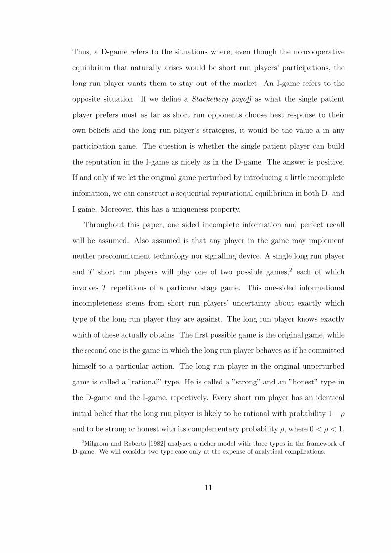
I study only two versions of game of great importance: with by > 0 > b0 in

common, either 0 > ay > a0, or a0 > ay > 0. All other cases are of little interest,

since the unique perfect equilibrium will be trivial, no matter what one sided

incomplete information in my sense there might be. I name the game with the first

type of payoff structure as an entry-deterrence game (D-game for short) and the

second as an entry-inducement game (I-game for short). A stage D-game has two

Nash equilibria [Out] and [In, Yes], but only the latter one is subgame perfect.1 On

the other hand, a one stage I-game has the unique Nash and perfect equilibrium

[Out]. Notice that, under the assumption of complete information, there is no

reason why the equilibrium of the T period repeated game becomes anything

other than the mere repetitions of the perfect equilibrium of the stage game.

1The other Nash equilibrium is subgame imperfect, since it can be supported only by anincredible off-the-equilibrium threat, i.e. player L’s no.

10

Thus, a D-game refers to the situations where, even though the noncooperative

equilibrium that naturally arises would be short run players’ participations, the

long run player wants them to stay out of the market. An I-game refers to the

opposite situation. If we define a Stackelberg payoff as what the single patient

player prefers most as far as short run opponents choose best response to their

own beliefs and the long run player’s strategies, it would be the value a in any

participation game. The question is whether the single patient player can build

the reputation in the I-game as nicely as in the D-game. The answer is positive.

If and only if we let the original game perturbed by introducing a little incomplete

infomation, we can construct a sequential reputational equilibrium in both D- and

I-game. Moreover, this has a uniqueness property.

Throughout this paper, one sided incomplete information and perfect recall

will be assumed. Also assumed is that any player in the game may implement

neither precommitment technology nor signalling device. A single long run player

and T short run players will play one of two possible games,2 each of which

involves T repetitions of a particuar stage game. This one-sided informational

incompleteness stems from short run players’ uncertainty about exactly which

type of the long run player they are against. The long run player knows exactly

which of these actually obtains. The first possible game is the original game, while

the second one is the game in which the long run player behaves as if he committed

himself to a particular action. The long run player in the original unperturbed

game is called a ”rational” type. He is called a ”strong” and an ”honest” type in

the D-game and the I-game, repectively. Every short run player has an identical

initial belief that the long run player is likely to be rational with probability 1−ρ

and to be strong or honest with its complementary probability ρ, where 0 < ρ < 1.

2Milgrom and Roberts [1982] analyzes a richer model with three types in the framework ofD-game. We will consider two type case only at the expense of analytical complications.

11

A useful solution concept to analyze these games with incomplete information is

the sequential equilibrium as developed in Kreps and Wilson [1982a].

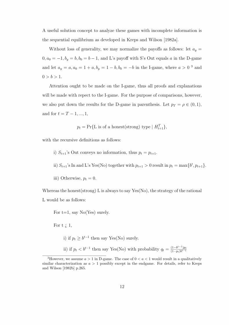
Without loss of generality, we may normalize the payoffs as follows: let ay =

0, a0 = −1, by = b, b0 = b− 1, and L’s payoff with S’s Out equals a in the D-game

and let ay = a, a0 = 1 + a, by = 1 − b, b0 = −b in the I-game, where a > 0 3 and

0 > b > 1.

Attention ought to be made on the I-game, thus all proofs and explanations

will be made with repect to the I-game. For the purpose of comparisons, however,

we also put down the results for the D-game in parenthesis. Let pT = ρ ∈ (0, 1),

and for t = T − 1, ..., 1,

pt = PrL is of a honest(strong) type | HTt+1,

with the recursive definitions as follows:

i) St+1’s Out conveys no information, thus pt = pt+1.

ii) St+1’s In and L’s Yes(No) together with pt+1 > 0 result in pt = maxbt, pt+1.

iii) Otherwise, pt = 0.

Whereas the honest(strong) L is always to say Yes(No), the strategy of the rational

L would be as follows:

For t=1, say No(Yes) surely.

For t ¿ 1,

i) if pt ≥ bt−1 then say Yes(No) surely.

ii) if pt < bt−1 then say Yes(No) with probability qt = (1−bt−1)pt

(1−pt)bt−1

3However, we assume a > 1 in D-game. The case of 0 < a < 1 would result in a qualitativelysimilar characterization as a > 1 possibly except in the endgame. For details, refer to Krepsand Wilson [1982b] p.265.

12

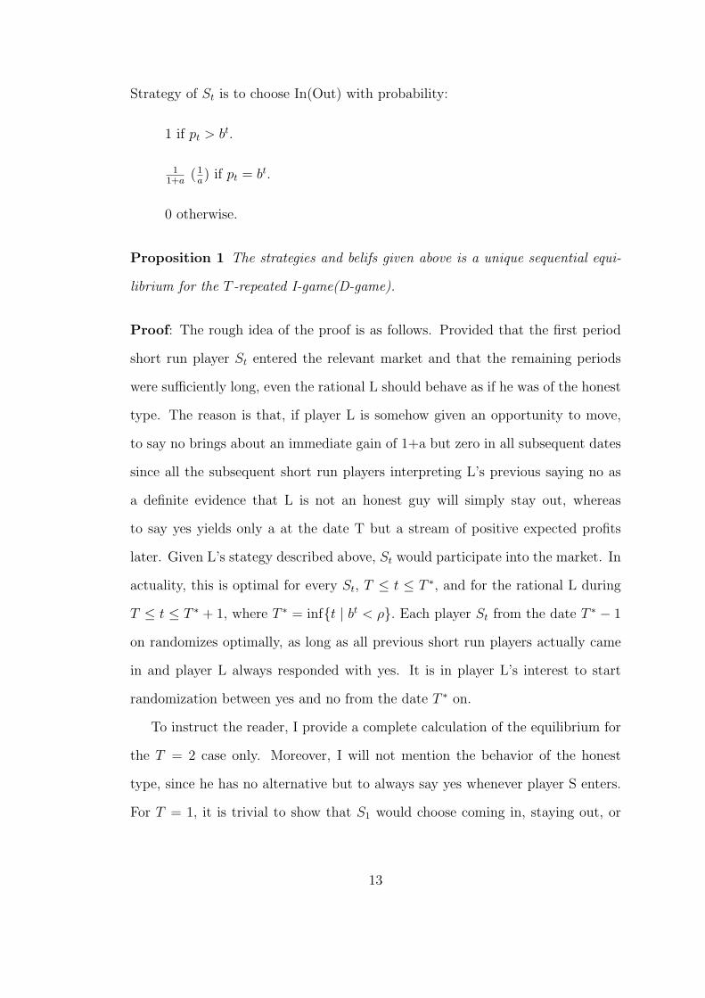
Strategy of St is to choose In(Out) with probability:

1 if pt > bt.

11+a

( 1a) if pt = bt.

0 otherwise.

Proposition 1 The strategies and belifs given above is a unique sequential equi-

librium for the T -repeated I-game(D-game).

Proof: The rough idea of the proof is as follows. Provided that the first period

short run player St entered the relevant market and that the remaining periods

were sufficiently long, even the rational L should behave as if he was of the honest

type. The reason is that, if player L is somehow given an opportunity to move,

to say no brings about an immediate gain of 1+a but zero in all subsequent dates

since all the subsequent short run players interpreting L’s previous saying no as

a definite evidence that L is not an honest guy will simply stay out, whereas

to say yes yields only a at the date T but a stream of positive expected profits

later. Given L’s stategy described above, St would participate into the market. In

actuality, this is optimal for every St, T ≤ t ≤ T ∗, and for the rational L during

T ≤ t ≤ T ∗ + 1, where T ∗ = inft | bt < ρ. Each player St from the date T ∗ − 1

on randomizes optimally, as long as all previous short run players actually came

in and player L always responded with yes. It is in player L’s interest to start

randomization between yes and no from the date T ∗ on.

To instruct the reader, I provide a complete calculation of the equilibrium for

the T = 2 case only. Moreover, I will not mention the behavior of the honest

type, since he has no alternative but to always say yes whenever player S enters.

For T = 1, it is trivial to show that S1 would choose coming in, staying out, or

13

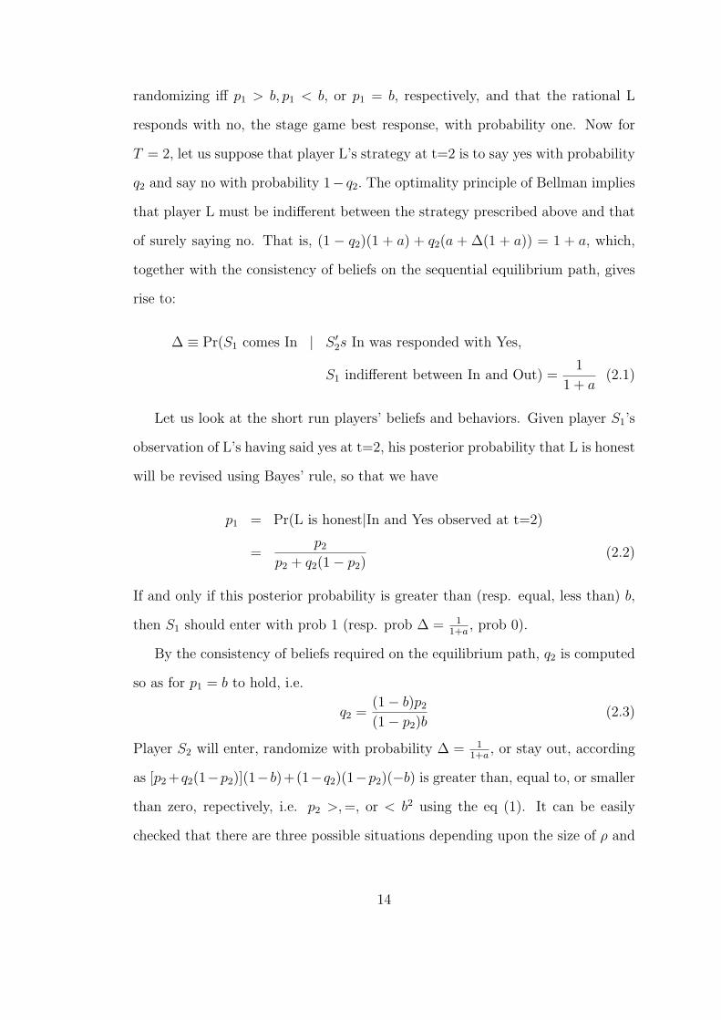
randomizing iff p1 > b, p1 < b, or p1 = b, respectively, and that the rational L

responds with no, the stage game best response, with probability one. Now for

T = 2, let us suppose that player L’s strategy at t=2 is to say yes with probability

q2 and say no with probability 1− q2. The optimality principle of Bellman implies

that player L must be indifferent between the strategy prescribed above and that

of surely saying no. That is, (1 − q2)(1 + a) + q2(a + ∆(1 + a)) = 1 + a, which,

together with the consistency of beliefs on the sequential equilibrium path, gives

rise to:

∆ ≡ Pr(S1 comes In | S ′2s In was responded with Yes,

S1 indifferent between In and Out) =1

1 + a(2.1)

Let us look at the short run players’ beliefs and behaviors. Given player S1’s

observation of L’s having said yes at t=2, his posterior probability that L is honest

will be revised using Bayes’ rule, so that we have

p1 = Pr(L is honest|In and Yes observed at t=2)

=p2

p2 + q2(1− p2)(2.2)

If and only if this posterior probability is greater than (resp. equal, less than) b,

then S1 should enter with prob 1 (resp. prob ∆ = 11+a

, prob 0).

By the consistency of beliefs required on the equilibrium path, q2 is computed

so as for p1 = b to hold, i.e.

q2 =(1− b)p2

(1− p2)b(2.3)

Player S2 will enter, randomize with probability ∆ = 11+a

, or stay out, according

as [p2 +q2(1−p2)](1−b)+(1−q2)(1−p2)(−b) is greater than, equal to, or smaller

than zero, repectively, i.e. p2 >, =, or < b2 using the eq (1). It can be easily

checked that there are three possible situations depending upon the size of ρ and

14

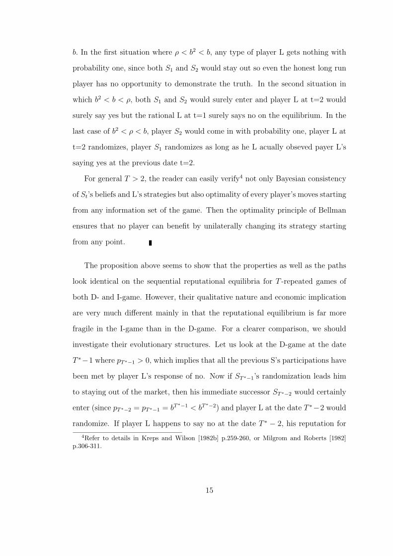
b. In the first situation where ρ < b2 < b, any type of player L gets nothing with

probability one, since both S1 and S2 would stay out so even the honest long run

player has no opportunity to demonstrate the truth. In the second situation in

which b2 < b < ρ, both S1 and S2 would surely enter and player L at t=2 would

surely say yes but the rational L at t=1 surely says no on the equilibrium. In the

last case of b2 < ρ < b, player S2 would come in with probability one, player L at

t=2 randomizes, player S1 randomizes as long as he L acually obseved payer L’s

saying yes at the previous date t=2.

For general T > 2, the reader can easily verify4 not only Bayesian consistency

of St’s beliefs and L’s strategies but also optimality of every player’s moves starting

from any information set of the game. Then the optimality principle of Bellman

ensures that no player can benefit by unilaterally changing its strategy starting

from any point.

The proposition above seems to show that the properties as well as the paths

look identical on the sequential reputational equilibria for T -repeated games of

both D- and I-game. However, their qualitative nature and economic implication

are very much different mainly in that the reputational equilibrium is far more

fragile in the I-game than in the D-game. For a clearer comparison, we should

investigate their evolutionary structures. Let us look at the D-game at the date

T ∗−1 where pT ∗−1 > 0, which implies that all the previous S’s participations have

been met by player L’s response of no. Now if ST ∗−1’s randomization leads him

to staying out of the market, then his immediate successor ST ∗−2 would certainly

enter (since pT ∗−2 = pT ∗−1 = bT ∗−1 < bT ∗−2) and player L at the date T ∗−2 would

randomize. If player L happens to say no at the date T ∗ − 2, his reputation for

4Refer to details in Kreps and Wilson [1982b] p.259-260, or Milgrom and Roberts [1982]p.306-311.

15

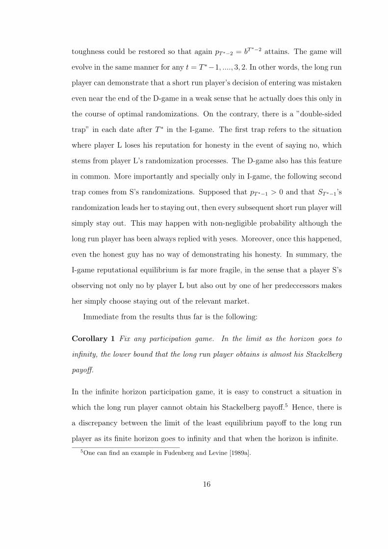
toughness could be restored so that again pT ∗−2 = bT ∗−2 attains. The game will

evolve in the same manner for any t = T ∗−1, ...., 3, 2. In other words, the long run

player can demonstrate that a short run player’s decision of entering was mistaken

even near the end of the D-game in a weak sense that he actually does this only in

the course of optimal randomizations. On the contrary, there is a ”double-sided

trap” in each date after T ∗ in the I-game. The first trap refers to the situation

where player L loses his reputation for honesty in the event of saying no, which

stems from player L’s randomization processes. The D-game also has this feature

in common. More importantly and specially only in I-game, the following second

trap comes from S’s randomizations. Supposed that pT ∗−1 > 0 and that ST ∗−1’s

randomization leads her to staying out, then every subsequent short run player will

simply stay out. This may happen with non-negligible probability although the

long run player has been always replied with yeses. Moreover, once this happened,

even the honest guy has no way of demonstrating his honesty. In summary, the

I-game reputational equilibrium is far more fragile, in the sense that a player S’s

observing not only no by player L but also out by one of her predeccessors makes

her simply choose staying out of the relevant market.

Immediate from the results thus far is the following:

Corollary 1 Fix any participation game. In the limit as the horizon goes to

infinity, the lower bound that the long run player obtains is almost his Stackelberg

payoff.

In the infinite horizon participation game, it is easy to construct a situation in

which the long run player cannot obtain his Stackelberg payoff.5 Hence, there is

a discrepancy between the limit of the least equilibrium payoff to the long run

player as its finite horizon goes to infinity and that when the horizon is infinite.

5One can find an example in Fudenberg and Levine [1989a].

16

2.3 Announcement and Commitment

A practical aspect that many examples of the I-game have in common may be

that, given a short run player’s participation into the relevant market, there is a

tradeoff between the long run player’s short term profit and the relevant short run

player’s payoff. Moreover, their payoffs are usually control variables the long run

player can determine. In a quality game, given a consumer’s decision to purchase

one unit of goods the monoplist wants to sell, a negative relationship between the

level of product quality and the monopolist’s short term profit seems to obviously

exist. In an asset market game as in Fudenberg and Levine [1989b], after some

investors or workers provide their assets or labors to the single patient capitalist,

a similar conflict may exist between returns to investors wage compensations to

the workers and profits to the capitalist.

To investigate this situation, we slightly modify the payoff structure. As before,

player St’s choosing an outside option yields nothing to both player L and himself.

Player St’s participation directly brings about −1 to himself and y to player L.

Here −1 that player St gets can be interpreted as disutility from consuming low

quality goods in a quality game and as value of financial assets provided to the

capitalist in an asset market game. The long run player decides whether to offer

a compensation 1+w to the short run player or not at all. We assume that player

L determines a level of w and that all the short run players somehow get to know

the precise value of w before the whole game begins.6 Presumably, a condition

that 1 + w > 0 must hold, since otherwise In is a dominated strategy for player

St,∀t, thus every St will simply stay out. On the other hand, player L has no

incentive to offer the gross compensation greater than y, so that y > 1 + w also

6This is not an innocuous assumption. Refer to Hart and Tirole [1988] for some resultswithout this restriction.

17

holds. Some reader might guess that player L has no incentive to offer more than

1 + ε, ∀ε > 0. This is wrong because a reduction of the compensation by player L

brings about not only benefits from directly raising his own share but also costs

from losing some customers who would have surely come in before.

As a prelimenary for the main result of this section, the reader can check the

following lemma by mimicking proofs of proposition 1:

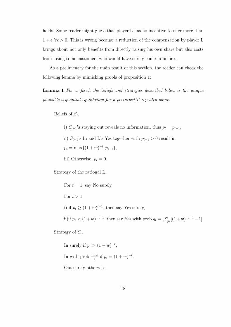
Lemma 1 For w fixed, the beliefs and strategies described below is the unique

plausible sequential equilibrium for a perturbed T -repeated game.

Beliefs of St.

i) St+1’s staying out reveals no information, thus pt = pt+1,

ii) St+1’s In and L’s Yes together with pt+1 > 0 result in

pt = max(1 + w)−t, pt+1,

iii) Otherwise, pt = 0.

Strategy of the rational L.

For t = 1, say No surely

For t > 1,

i) if pt ≥ (1 + w)t−1, then say Yes surely,

ii)if pt < (1+w)−t+1, then say Yes with prob qt = pt

1−pt[(1+w)−t+1−1].

Strategy of St.

In surely if pt > (1 + w)−t,

In with prob 1+wy

if pt = (1 + w)−t,

Out surely otherwise.

18

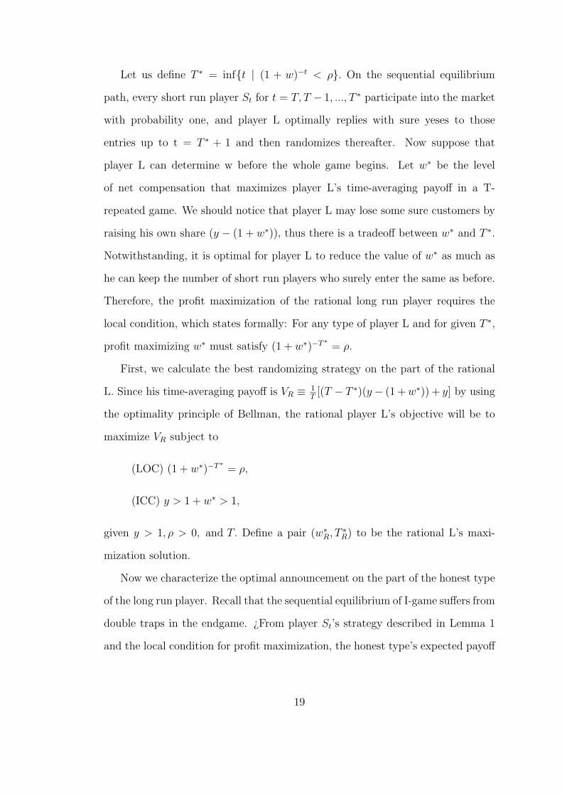
Let us define T ∗ = inft | (1 + w)−t < ρ. On the sequential equilibrium

path, every short run player St for t = T, T − 1, ..., T ∗ participate into the market

with probability one, and player L optimally replies with sure yeses to those

entries up to t = T ∗ + 1 and then randomizes thereafter. Now suppose that

player L can determine w before the whole game begins. Let w∗ be the level

of net compensation that maximizes player L’s time-averaging payoff in a T-

repeated game. We should notice that player L may lose some sure customers by

raising his own share (y − (1 + w∗)), thus there is a tradeoff between w∗ and T ∗.

Notwithstanding, it is optimal for player L to reduce the value of w∗ as much as

he can keep the number of short run players who surely enter the same as before.

Therefore, the profit maximization of the rational long run player requires the

local condition, which states formally: For any type of player L and for given T ∗,

profit maximizing w∗ must satisfy (1 + w∗)−T ∗= ρ.

First, we calculate the best randomizing strategy on the part of the rational

L. Since his time-averaging payoff is VR ≡ 1T[(T − T ∗)(y− (1 + w∗)) + y] by using

the optimality principle of Bellman, the rational player L’s objective will be to

maximize VR subject to

(LOC) (1 + w∗)−T ∗= ρ,

(ICC) y > 1 + w∗ > 1,

given y > 1, ρ > 0, and T. Define a pair (w∗R, T ∗

R) to be the rational L’s maxi-

mization solution.

Now we characterize the optimal announcement on the part of the honest type

of the long run player. Recall that the sequential equilibrium of I-game suffers from

double traps in the endgame. ¿From player St’s strategy described in Lemma 1

and the local condition for profit maximization, the honest type’s expected payoff

19

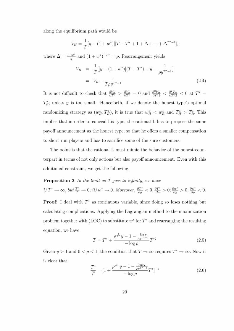
along the equilibrium path would be

VH =1

T[y − (1 + w∗)][T − T ∗ + 1 + ∆ + ... + ∆T ∗−1],

where ∆ = 1+w∗

yand (1 + w∗)−T ∗

= ρ. Rearrangement yields

VH =1

T[[y − (1 + w∗)](T − T ∗) + y − 1

ρyT ∗−1]

= VR −1

TρyT ∗−1(2.4)

It is not difficult to check that ∂VH

∂T ∗ > ∂VR

∂T ∗ = 0 and ∂2VH

∂T ∗2< ∂2VH

∂T ∗2< 0 at T ∗ =

T ∗R, unless y is too small. Henceforth, if we denote the honest type’s optimal

randomizing strategy as (w∗H , T ∗

H), it is true that w∗H < w∗

R and T ∗H > T ∗

R. This

implies that,in order to conceal his type, the rational L has to propose the same

payoff announcement as the honest type, so that he offers a smaller compensation

to short run players and has to sacrifice some of the sure customers.

The point is that the rational L must mimic the behavior of the honest coun-

terpart in terms of not only actions but also payoff announcement. Even with this

additional constraint, we get the following:

Proposition 2 In the limit as T goes to infinity, we have

i) T ∗ →∞, but T ∗

T→ 0; ii) w∗ → 0. Moreover, ∂T ∗

∂y< 0, ∂T ∗

∂ρ> 0; ∂w∗

∂y> 0, ∂w∗

∂ρ< 0.

Proof: I deal with T ∗ as continuous variable, since doing so loses nothing but

calculating complications. Applying the Lagrangian method to the maximization

problem together with (LOC) to substitute w∗ for T ∗ and rearranging the resulting

equation, we have

T = T ∗ +ρ

1T∗ y − 1− log y

ρyT∗−1

− log ρT ∗2 (2.5)

Given y > 1 and 0 < ρ < 1, the condition that T →∞ requires T ∗ →∞. Now it

is clear that

T ∗

T= [1 +

ρ1

T∗ y − 1− log yρyT∗−1

− log ρT ∗]−1 (2.6)

20

thus

limT→∞

T ∗

T= lim

T ∗→∞

T ∗

T= 0,

together with limT→∞ T ∗ = ∞. We proved i).

On the other hand, taking log to both sides of (LOC) and rearranging yields

w∗ = ρ−1T∗ − 1, thus limT→∞ w∗ = limT ∗→∞ w∗ = 0. The second part ii) is also

done.

The proposition above implies that, as the horizon gets larger and larger, the

number of short run players who optimally randomize near the end of the game

also should be controlled larger, while its relative proportion gets negligible. In

other words, the proportion of sure customers who enter the market with proba-

bility one monotonically approaches to unity. In addition, the long run player can

optimally reduce the amount of net compensation that provides to some short run

players incentives to participate into the relevant market. The second part shows

some comparative statics which states that the optimal net compensation become

smaller as the horizon gets larger, as shortrun player’s probability assessment that

player L is of the honest type gets bigger, and as the total revenue to player L gets

smaller. As a consequence, the long run player is able to obtain almost extensive

form Stackelberg payoff for sufficiently long horizon T. Moreover, in the limit as

the horizon T approaches to infinity, the ε-first-best is indeed attainable.

2.4 Final Remarks

Consider repeated games in which a single patient player plays against a finite se-

quence of short run opponents. As a particular deterministic stage game in which

short run players move first in each stage game, a participation game may have

many practical applications, such as entry-deterrence behavior by an incumbent,

a quality choice by a monopolist, a debt decision by a less developed country, etc.

21

I study charaterizations and properties of the sequential equilibrium in finitely-

repeated participation games only by introducing a small perturbations into the

original game. I show that reputation effects play an important role in any par-

ticipation game as almost nicely as in any simultaneous move game. This is a

surprising counterargument to the common view that the single patient player

is not able to acquire or maintain a reputation in finitely repeated I-games. As

a limit of finitly repeated participation games, the reputational equilibrium of

the infinitely repeated game is also well characterized. Therefore, the fact that

the long run player can obtain his Stackelberg payoff was shown, although the

Stackelberg payoff here is differently calculated from that of simultaneous move

games. These consequences are robust to a model modification where the long

run player announces the payoff structure, which puts an additional contraint on

the behavior of rational type.

An important problem that is worth being pursued will be to calculate the

lower bound that the long run player can obtain on any sequential equilibrium of

general extensive form game in the limit as the horizon grows.7

7Schmidt [1990, 1992] analyzes repeated bargaining problem and games with conflictinginterest.

22

Figure 2.1: Product Quality Game

Figure 2.2: Entry Deterrence Game

23

Figure 2.3: Participation Game

24

Chapter 3

Adjustment Dynamics withPatient Players

25

3.1 Introduction

In this paper, we analyze a game played by randomly and anonymously matched

players from a large population. Players face a perfect foresight deterministic

dynamic process with costly adjustment. The class of games we study are sym-

metric binary action mutiperson coordination games with two strict Pareto-ranked

Nash equilibria.1 Consideration of these games is motivated by the simple game-

theoretic issue of selection in games with multiple equilibria in which existing

refinements are powerless. For instance, many of the stringent solution concepts

proposed in the literature, such as the strategic stability of Kohlberg and Mertens

[1986], are silent concerning the selection among several strict Nash equilibria.

Furthermore, some recent studies on learning and evolution have also addressed

the question of how a particular equilibrium will emerge in a dynamic context.2

Although some convergence results are obtained, these studies do not offer an

equilibrium selection criterion, since in these models all strict Nash equilibria

share the same dynamic properties.

One approach for resolving this indeterminacy is to consider an actual adjust-

ment process which operates in real time, and to see what limit outcomes if any

might appear. For example, we allow players to have the opportunity from time

to time to revise their choices given what their opponents are currently doing,

and given the “correct” expectation about the future play of the game (namely,

perfect foresight). If this continuous revision process settles down to a unique

outcome, then this outcome should be the analyst’s prediction of how the game

1This class of games represents, in a stylized fashion, the types of interactions prevalent innetwork externalities such as compatibility of computer software, video tapes, typewriter key-boards, and language, as well as many recent Keynesian macroeconomic models of coordinationfailures, geographical formation of core and periphery (Krugman [1991]).

2A partial list of this literature includes Jordan [1991], Fudenberg and Kreps [1992a], Canning[1992], Milgrom and Roberts [1990, 1991], and Fudenberg and Levine [1992a, b].

26

might be played. Therefore, this approach has the potential of explaining how

an equilibrium is attained, and of singling out a unique equilibrium in situations

where the underlying static game has multiple Nash equilibria.

This avenue has been explored in recent adaptive or evolutionary formulations,

3 most of which have asserted that the limit dynamic equilibrium outcome coincide

with Harsanyi and Selten’s [1988] static notion of risk dominance. The limit

behavior of Blume’s [1] dynamic process with respect to parametric changes that

make strategy revisions a best response is shown to give rise to the same outcome

as risk dominance selection in coordination games. Kandori, Mailath, and Rob

[1992] consider evolutionary models for a finite population in discrete time with

constant flow of mutations, which generate Markov processes in the behavioral

pattern. Fudenberg and Harris [1992] study a version of the replicator dynamic

in continuous time for a large population. In this paper, the random perturbation

of the system is introduced by a Brownian motion. These last two papers show

the same result: for 2 × 2 games, as the mutation rate and noise go to zero,

the distribution becomes concentrated on the risk dominant equilibrium. Lastly,

Matsui and Matsuyama [1991]—from which the present paper borrows heavily—

shows an equivalence between risk dominance and dynamic stability in a two

person bimatrix game of common interests.

The results of this paper cast strong doubt on the conjectured equivalence be-

tween the limit dynamic outcome and risk dominance. We will show that, for the

Matsui and Matsuyama approach, these two notions “happen” to coincide only in

3This is nothing but one strand of numerous frameworks. Other popular and interesting ap-proaches, which specifically study games with multiple equilibria, are fictitious learning (Krishna[1992]), learning with bounded memory or finite automata (Aumann and Sorin [1989]; Binmoreand Samuelson [1992]), Turing machine learning under computability (Anderlini and Sabourian[1991] and references therein), and so on. Another game of great importance is prisoner’sdilemma, which Young and Foster [1991] analyzes using stochastic evolutionary dynamics, andNowak and May [1992], Glance and Huberman [1992], and references therein provide computersimulation results in machine learning framework.

27

the two person bimatrix game. First, we will fully characterize the dynamic equi-

librium outcome in terms of group size and a friction parameter which depends

positively on the discount rate of players and negatively on the chance of their ac-

tion switches. To say the friction disappears implies that players are very patient,

or that each player can revise his choice whenever he wants. On the other hand,

to say the friction grows without bound implies that players are myopic, or that

they choose strategies once and for all. A state is said to be globally attractive

if there exists an equilibrium path that reaches or converges to that state from

any initial condition. It is shown that, in the limit as the friction vanishes, either

everyone’s playing one action or everyone’s playing the other will be the globally

attractive state, depending upon the payoff matrix.

Surprisingly, the limit as the friction approaches zero turns out to coincide with

Carlsson and Van Damme’s [1990, 1991] notion of equilibrium selection through

perturbation of the original game. The original game is perturbed in such a way

that each player receives a private signal about the payoffs, but is unable to fully

disentangle the true payoff realization from one’s private noise. Lack of com-

mon knowledge among players makes it possible for strictly dominated strategies

to exert an influence. This fact suggests that, to solve the resulting incomplete

information game, we must use iterative elimination of strictly dominated strate-

gies. When common knowledge about payoffs becomes arbitrarily perfect among

players, the result of iterative strict dominance prescribes that all players play

either one or the other action, depending on the payoff matrix of the original

unperturbed game. The major argument of this paper is that this globally at-

tractive dynamic outcome, in the limit as the friction disappears, coincides with

equilibrium selection based on a global perturbation approach.

As verified by Matsui [1992], the opposite limit as players become myopic is

28

closely related to a version of evolutionary stability, attributed to Swinkels [1992a].

Note that the evolutionarily stable strategy is defined as a strategy distribution

which is robust against a once-and-for-all invasion by a small number of mutants.

For this limit dynamic, the payoff matrix does not matter at all and only the ini-

tial fraction of each action type does. Such indetermincy is resolved if we perturb

the dynamical system with a constant flow of mutations and experimentations.

The idea behind mutations is to test the stability of states by repeatedly sub-

jecting them to disturbances, and observing to which states the society tends to

return. My companion paper [19] not only characterizes the long run ergodic

distribution in the limit as the probability of mutations vanishes, which suggests

a criterion for selecting among multiple strict Nash equilibria; it also clarifies the

link between the features of the underlying dynamics and the static equilibrium

selection. Roughly speaking, the long run state obtained with patient players cor-

responds to the static equilibrium assuming correlated play of opponents, while

the long run state obtained with myopic players corresponds to the static equilib-

rium selection predicted by independent play of one’s opponents.

The present paper may also have substantial implications with regard to re-

cently developed experimental results by Van Huyck et al. [1990, 1991] on coor-

dination failure, and by Cooper et al. [1990] on the predictability of Nash equi-

librium. In particular, we provide theoretical and numerical evidence that is

consistent with the following observations:

• weak dominance,

• a wide dispersion of initial effort choices,

• a trend to drift in small group treatments,

• a rapid convergence to the Pareto-worst Nash equilibrium regardless of ini-

tial strategic uncertainty when the group size is large and the summary

29

statistic affecting each player’s payoff is the minimum effort choice among

the group (i.e. large group minimum treatment),

• a strong history dependency in large group median treatments,

• and Pareto efficiency in pure coordination problems.

To recapitulate, coordination failure and history dependency are the most remark-

able features, respectively, under minimum and median rule, when the group size

is large.

The balance of the paper is organized as follows. Section 3.2 offers an intu-

itive exposition of the basic idea with a simple example. Section 3.3 formally

defines the game of interest. Section 3.4 sets up the dynamic model and then

characterizes its dynamic equilibrium outcomes. Section 3.5 contains calculations

two important static equilibrium selection concepts, namely global perturbation

and risk dominance. This same section proves the equivalence between the limit

adjustment dynamic outcome and the static equilibrium selection based on global

perturbation. Section 3.6 proves a strong result that, in any –symmetric or asym-

metric – 2 × 2 game, the limit dynamic equilibrium outcome coincides with the

selection based on global perturbation. This is also true even if the speed of ad-

justments are different, as long as the proportion between them is fixed in the

limit. Section 3.7 studies two interesting subclasses of the original game, that

is, pure coordination and stag hunt games. Section 3.8 offers numerical evidence

within the framework of the stag hunt game used in experimental studies. The

last section concludes with some suggestions for future research.

3.2 An Exposition

Consider the following highly stylized game. A forest is inhabited by a stag and a

number of hares. There are n identical hunters that simultaneously and without

30

communication have to choose between hunting a stag or a hare. If a player

decides to hunt for a hare, his payoff is $x no matter what the other hunters

may choose. If the player decides to pursue a stag then his payoff is determined

not only by his own choice but by the actions of others, summarized by a simple

statistic. Roughly speaking, stag hunting is successful only when enough of the

hunters cooperate. Under a “minimum rule,” even a single defection from full

cooperation results in a failure. Under a “median rule,” the cooperation of 50%

of the hunters is sufficient for a successful stag hunt. We further specify that a

successful stag hunt yields $10 to each of the participants, whereas a failure brings

about nothing. The normal form of this game is called the stag hunt game, the

two and three-player version of which are depicted in Figure 3.1 and Figure 3.2.

We first study the dynamic evolution of the social equilibrium played by a large

population. Each hunter is randomly and repeatedly matched with (n− 1) other

players to play the stage stag hunt game anonymously. Players are fully rational,

maximizing their discounted average expected payoff, with the dynamic path on

which they condition their expected payoffs perfectly foreseen. However, there is

friction: not every player is able to switch his own action every period. While this

assumption is stylized, it can be interpreted as a transaction cost. For example, it

could be the cost of switching from rabbit traps to hunting rifles. All the hunters

are assumed to observe what fraction of hunters in the society as a whole are

choosing between hares and stags. Given the opportunity to switch, each hunter

chooses an action that maximizes his expected utility conditional on the correct

expectation of the future play of the game. The dynamic equilibrium outcome

is fully characterized as a function of group size n, and the effective discount

rate ρ. The effective discount rate takes into account both the real-time discount

rate and the cost to switching actions. The long run steady state of the social

31

equilibrium must end up with either everyone hunting stag or everyone hunting

hares, depending upon the payoff x and the initial fraction of stag hunters. While

not regretting their individual choice in either equilibria, people in hare hunting

society are nevertheless worse off than those in stag hunting society. Defection

by a single individual or a negligible number of agents is simply in vain. In other

words, all hunters may be playing a best response, but there is a chance that these

best responses implement a Pareto-inferior equilibrium.

To take a concrete example, let n = 2 and ρ = 12. It can be shown that the

“good” stag (“bad” hare) equilibrium can result regardless of the initial popu-

lation fraction of hare hunters, if the sure return to rabbit hunting x, is smaller

than $4 (greater than $6).4 In the case where x is between $4 and $6, the his-

torical accident with regard to the initial fraction of hunter types plays a crucial

role in determining exactly the long run equilibrium. Now, as players become

more patient in the sense that ρ approaches to zero, the middle region of history

dependency shrinks. There is a single limiting threshold value of x equal to the

average payoff of the stag hunt under the assumption that the possibility of each

opponent’s hunting stag is equally likely. According to this assumption, since the

probability that the opponent chooses stag and the probability that his opponent

chooses hare are equal, the threshold is 12× 10 + 1

2× 0 = $5. To compare with

another set of parameters, let n = 3 and ρ = 12, under a minimum rule. Then

the history dependent region would be between $2.28 and $4.28, which shrinks to

an infinitesimal area around 13× 10 + 2

3× 0 = $3.33, if people care very much

about their future. Roughly put, in the limit as people are extremely patient,

the society eventually settles down on the stag (hare) equilibrium if x is smaller

(greater) than $3.33. For a last example with n = 7 under a median rule, it is

4The reader will have to trust me for the accuracy of these numbers, which are calculatedusing Eqs. (3.5)–(3.8) derived in Section 3.4.

32

easy to check the limit critical value equals 47× 10 + 3

7× 0 = $5.71.

We now turn to Harsanyi and Selten’s [1988] notion of risk dominance. The

definition of risk dominance is based on a hypothetical process of expectation

formation starting from an initial situation where it is common knowledge that

either the stag equilibrium or the hare equilibrium must be the solution without

knowing which one is the solution. Consider a process in which players first, on

the basis of a preliminary theory, form priors on the strategies of their opponents.

The preliminary theory can be summarized as follows: (i) Each player i believes

that either all the other players hunt stag with a subjective probability zi or all

other players hunt hares with its complementary probability; (ii) each player i

plays his best response to this belief; (iii) the zi are independently and uniformly

distributed on [0, 1]. Unfortunately this naive theory will not work since this best

reply strategy combination will generally not be an equilibrium point of the game,

and therefore it cannot be the outcome chosen by a rational outcome selection

theory. The second-order best reply to the first-order vector is iteratively calcu-

lated. Thereafter, players gradually adapt their prior expectations to the final

equilibrium expectations by means of a tracing procedure. As the tracing proce-

dure progresses, both the prior vector and the best response strategy combination

are subjected to systematic and continuous transformations until both of them

finally converge to a specific equilibrium of the game. Thus at the end of the trac-

ing procedure both the players’ actual strategy plans and expectations about each

other’s strategy plans will correspond to the same equilibrium point, representing

the risk dominant outcome.

Fortunately, the tracing procedure can be accomplished in one round in the

present stag hunt game. Consider the n = 2 case. According to steps (i) and (ii)

33

of the preliminary theory, hunter i chooses stag if:

zi × 10 + (1− zi)× 0 > x or zi >x

10

where i = 1, 2. Using step (iii), player i knows that his opponent chooses stag with

probability (1 − x10

) and hare with the complementary probability x10

, therefore

the prior must be revised to the posterior (1− x10

). Now player i optimally hunts

stag if

(1− x

10)× 10 +

x

10× 0 > x or x < $5.

We conclude that the stag hunt risk dominates hare catching if x < $5 and

vice-versa. For another example, let n = 3 under a minimum rule. Following

the steps described above suggests that the critical x value be the solution to

10 × (1 − x10

)2 + 0 × [1 − (1 − x10

)2] = x, so that risk dominance selects stag if

x < $3.82.

Finally we examine Carlsson and Van Damme’s [1990, 1991] notion of global

perturbation. It is based on the idea that players are uncertain about the payoffs

of the game. Trembling the game is made in such a way that payoffs are almost

but not perfectly common knowledge, and that there is a chance that each of the

actions can be a dominated strategy. To be specific, assume that the true number

of hares is uncertain. One extreme possibility is that no rabbit might be available

so that hare hunting only incurs an effort cost, while the other extreme possibility

is that the forest might be indeed crowded with rabbits so that even a successful

stag hunt fares worse than the hare hunt. More formally, there is a small but non-

negligible probability that x < 0 in which rabbit hunting is strictly dominated,

and x > $10 in which stag hunting is strictly dominated. Each hunter receives

a private signal that provides an unbised estimate of the true common value x,

but the signals are noisy so the true value of x will not be common knowledge.

34

The player then chooses whether to hunt stag or hare. Assume that the noise

can be at most $0.50. For instance, if the true value of x is $5.50, then all the

private signals must be somewhere between $5 and $6 from an outsider’s point of

view. Imagine a situation in which a particular hunter i just observes his private

signal xi equal to $5.50. Even if he knows, upon having observed $5.50, that the

true x lies between $5 and $6 and that all the other xj’s are between $4.50 and

$6.50, this is in fact not common knowledge to hunters i and j. Now suppose that

hunter j observes xj = $4.50. Hunter j knows that the true x lies between $4

and $5, and xi lies between $3.50 and $5.50. The problem is that hunter i does

not know that hunter j knows that his xi lies in the interval [$3.50, $5.50]. Lack

of common knowledge expands all the way down, and therefore enables remote

areas of dominated strategies where x is negative or greater than $10 to exert an

influence. This argument may well apply to all the other less extreme realizations

of xj in the interval [$4.50, $6.50], say $5.70 instead of $4.50, and any smaller

size of the maximum noise, say a dime or a penny instead of 50 cents. Later

we will show that equilibrium can be characterized using iterative elimination of

strictly dominated strategies, and that it possesses a cutoff property. Finally, we

are interested in what happens with the payoff realization that corresponds to the

original game.

Take the n = 2 game. As was suggested, we maintain the assumption that no

player will choose strictly dominated strategies. Hunter i will certainly choose stag

if the secure return from catching hare is negative, i.e. x < 0. Since the expected

true value of x conditional on his private signal xi is simply xi because of unbi-

asedness, player i knows that stag is strictly dominant at each such observation.

Consider xi to be slightly above zero. Notice that, with the additional assumption

that the private signal is uniformly distributed around the true common value of

35

x is imposed, the probability that your xj is bigger than my xi does not depend

upon xi, thus the conditional probability must always be half. Player i knows

that his opponent j will hunt stag if xj < 0, hence i’s payoff if he hunts stag at xi

would be approximately 12× 10 + 1

2× 0 = $5. As an astute reader might see,

the process of eliminating strictly dominated strategies ends up in one iteration

for stag hunt games. In other words, the same logic applies not only to an xi

slightly above zero, but also to any xi below $5. Since the expected payoff from

hare hunting is xi, we conclude that each hunter should hunt a stag (hare) if his

private signal about the secure return form hunting hares is smaller (larger) than

$5. For example with n = 3 under a minimum rule, it can be similarly calculated

that a hunter should choose a hare only when his private signal is smaller than

13× 10 + 2

3× 0 = $3.33.

Table 3.1 provides the cutoff values calculated for the limit adjustment dy-

namic outcome, risk dominance, and global perturbation in the case of minimum

and median rules when the number of players are n = 2, 3, 15, 99.5 The reader

may be aware that the dynamic equilibrium outcome selection in the limit as the

effective discount rate ρ goes to zero coincides with the static equilibrium selection

based on global perturbation but not of risk dominace. This is not by chance! We

will verify this equivalence in general coordination games.

3.3 The Game

We consider a symmetric n-person coordination game with binary actions, denoted

High (H) and Low (L). The normal form game denoted by G(n, Π) has 2n number

5It is interesting to note that under the minimum rule, global perturbation is more conserva-tive than risk dominance, in the sense that there is a subset of x such that risk dominance selectsthe risky Pareto-superior choice while global perturbation prescribes the secure Pareto-inferioraction. This observation implies that coordination failures are more severe from the viewpointof global perturbation than of risk dominance.

36

of cells, but due to symmetry only 2n cells need to be taken into account. Consider

a strategy profile in which k agents choose H with the remaining (n − k) agents

choosing L; we denote πHk and πL

n−k to be the payoff for a player taking H and

L respectively, where k = 1, 2, . . . , n. Let a vector Πζ = (πζ1, π

ζ2, . . . , π

ζn), for

ζ = H, L, and Π = (ΠH , ΠL) ∈ <2n. The game of interest belongs to:

Ω ≡

Π ∈ <2n | πζk+1 ≥ πζ

k, ∀ ζ, ∀ k with strict inequality for some k;

πHn > πL

1 , πLn > πH

1 ; πHn ≥ πL

n

. (3.1)

The first set of inequalities in Eq. (3.1) imply that a player taking a particular

action is no worse off when the number of opponents taking the same action

increases. The next two inequalities require that everyone playing a common

action is a strict Nash equilibrium. The last inequality means that the equilibrium

where everyone plays H, denoted H, is better than where everyone plays L, denoted

L. Figure 3.2 depicts an example of a three-person coordination game with H is

stag and L is hare. Now the following preliminary result is straightforward:

Lemma 2 If Π ∈ Ω then the only pure strategy equilibria of G(n, Π) are two strict

Nash, viz. H and L.

Proof It suffices to show that none of k = 1, 2, . . . , n− 1 satisfies both πLn−k >

πHk+1 and πH

k > πLn−k+1, since otherwise the pure strategy profile of k players

choosing H and (n− k) players choosing L would be Nash. Adding the above two

inequalities yields

−(πLn−k+1 − πL

n−k) > πHk+1 − πH

k

which contradicts the definition of the Ω set.

Any of the Nash refinements, including the strategic stability of Kohlberg and

Mertens, is powerless in selecting between these two strict Nash equilibria. Pareto

efficiency is compatible with equilibrium play, so neither an incentive problem nor

37

conflict exists. However, it is not clear whether players will be able to reach this

outcome in a noncooperative situation where no direct communication is allowed.

In short, strategic uncertainty matters.

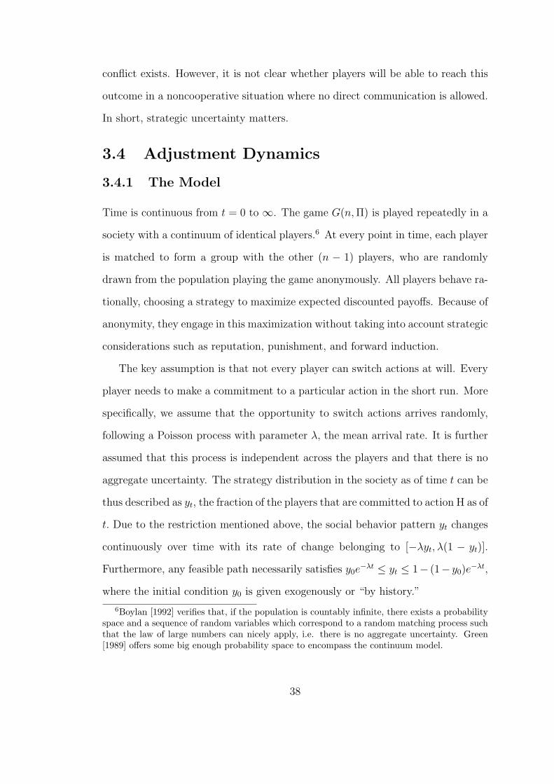
3.4 Adjustment Dynamics

3.4.1 The Model

Time is continuous from t = 0 to ∞. The game G(n, Π) is played repeatedly in a

society with a continuum of identical players.6 At every point in time, each player

is matched to form a group with the other (n − 1) players, who are randomly

drawn from the population playing the game anonymously. All players behave ra-

tionally, choosing a strategy to maximize expected discounted payoffs. Because of

anonymity, they engage in this maximization without taking into account strategic

considerations such as reputation, punishment, and forward induction.

The key assumption is that not every player can switch actions at will. Every

player needs to make a commitment to a particular action in the short run. More

specifically, we assume that the opportunity to switch actions arrives randomly,

following a Poisson process with parameter λ, the mean arrival rate. It is further

assumed that this process is independent across the players and that there is no

aggregate uncertainty. The strategy distribution in the society as of time t can be

thus described as yt, the fraction of the players that are committed to action H as of

t. Due to the restriction mentioned above, the social behavior pattern yt changes

continuously over time with its rate of change belonging to [−λyt, λ(1 − yt)].

Furthermore, any feasible path necessarily satisfies y0e−λt ≤ yt ≤ 1− (1− y0)e

−λt,

where the initial condition y0 is given exogenously or “by history.”

6Boylan [1992] verifies that, if the population is countably infinite, there exists a probabilityspace and a sequence of random variables which correspond to a random matching process suchthat the law of large numbers can nicely apply, i.e. there is no aggregate uncertainty. Green[1989] offers some big enough probability space to encompass the continuum model.

38

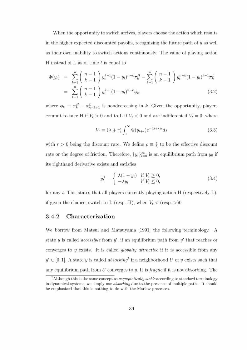
When the opportunity to switch arrives, players choose the action which results

in the higher expected discounted payoffs, recognizing the future path of y as well

as their own inability to switch actions continuously. The value of playing action

H instead of L as of time t is equal to

Φ(yt) =n∑

k=1

(n− 1k − 1

)yk−1

t (1− yt)n−kπH

k −n∑

k=1

(n− 1k − 1

)yn−k

t (1− yt)k−1πL

k

=n∑

k=1

(n− 1k − 1

)yk−1

t (1− yt)n−kφk, (3.2)

where φk ≡ πHk − πL

n−k+1 is nondecreasing in k. Given the opportunity, players

commit to take H if Vt > 0 and to L if Vt < 0 and are indifferent if Vt = 0, where

Vt ≡ (λ + r)∫ ∞

0Φ(yt+s)e

−(λ+r)sds (3.3)

with r > 0 being the discount rate. We define ρ ≡ rλ

to be the effective discount

rate or the degree of friction. Therefore, yt∞t=0 is an equilibrium path from y0 if

its righthand derivative exists and satisfies

y+t =

λ(1− yt) if Vt ≥ 0,−λyt if Vt ≤ 0,

(3.4)

for any t. This states that all players currently playing action H (respectively L),

if given the chance, switch to L (resp. H), when Vt < (resp. >)0.

3.4.2 Characterization

We borrow from Matsui and Matsuyama [1991] the following terminology. A

state y is called accessible from y′, if an equilibrium path from y′ that reaches or

converges to y exists. It is called globally attractive if it is accessible from any

y′ ∈ [0, 1]. A state y is called absorbing7 if a neighborhood U of y exists such that

any equilibrium path from U converges to y. It is fragile if it is not absorbing. The

7Although this is the same concept as asymptotically stable according to standard terminologyin dynamical systems, we simply use absorbing due to the presence of multiple paths. It shouldbe emphasized that this is nothing to do with the Markov processes.

39

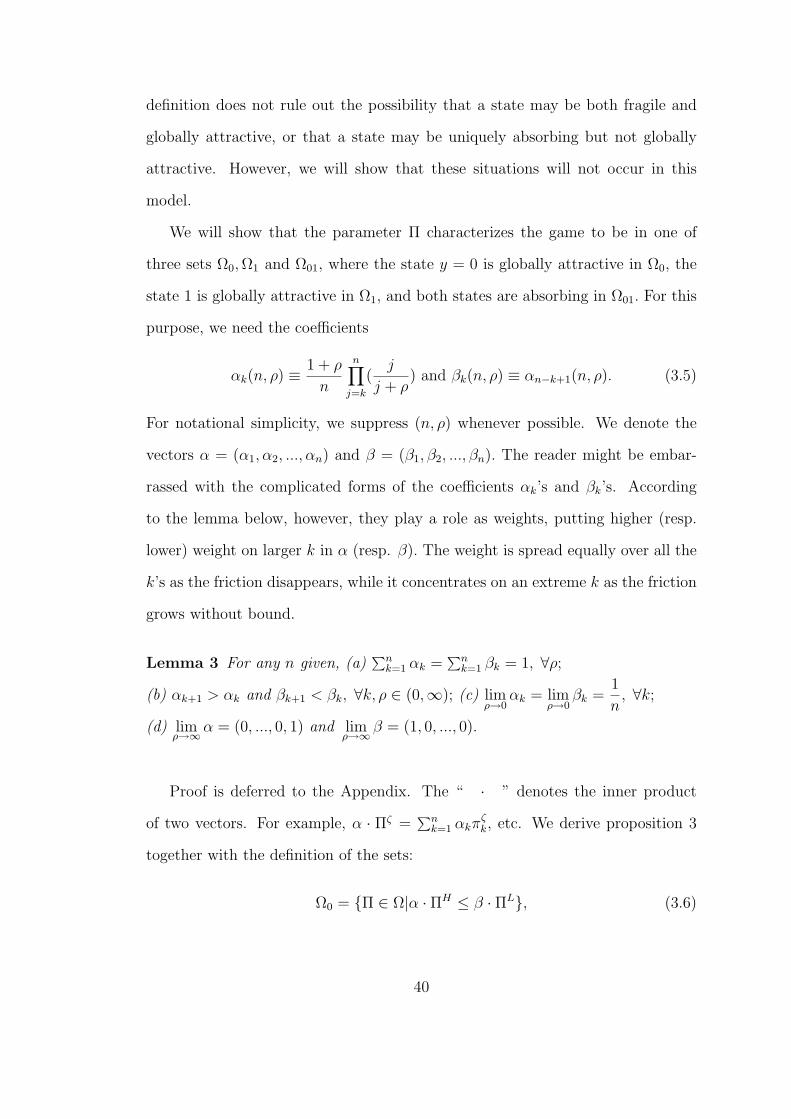
definition does not rule out the possibility that a state may be both fragile and

globally attractive, or that a state may be uniquely absorbing but not globally

attractive. However, we will show that these situations will not occur in this

model.

We will show that the parameter Π characterizes the game to be in one of

three sets Ω0, Ω1 and Ω01, where the state y = 0 is globally attractive in Ω0, the

state 1 is globally attractive in Ω1, and both states are absorbing in Ω01. For this

purpose, we need the coefficients

αk(n, ρ) ≡ 1 + ρ

n

n∏j=k

(j

j + ρ) and βk(n, ρ) ≡ αn−k+1(n, ρ). (3.5)

For notational simplicity, we suppress (n, ρ) whenever possible. We denote the

vectors α = (α1, α2, ..., αn) and β = (β1, β2, ..., βn). The reader might be embar-

rassed with the complicated forms of the coefficients αk’s and βk’s. According

to the lemma below, however, they play a role as weights, putting higher (resp.

lower) weight on larger k in α (resp. β). The weight is spread equally over all the

k’s as the friction disappears, while it concentrates on an extreme k as the friction

grows without bound.

Lemma 3 For any n given, (a)∑n

k=1 αk =∑n

k=1 βk = 1, ∀ρ;

(b) αk+1 > αk and βk+1 < βk, ∀k, ρ ∈ (0,∞); (c) limρ→0

αk = limρ→0

βk =1

n, ∀k;

(d) limρ→∞

α = (0, ..., 0, 1) and limρ→∞

β = (1, 0, ..., 0).

Proof is deferred to the Appendix. The “ · ” denotes the inner product

of two vectors. For example, α · Πζ =∑n

k=1 αkπζk, etc. We derive proposition 3

together with the definition of the sets:

Ω0 = Π ∈ Ω|α · ΠH ≤ β · ΠL, (3.6)

40

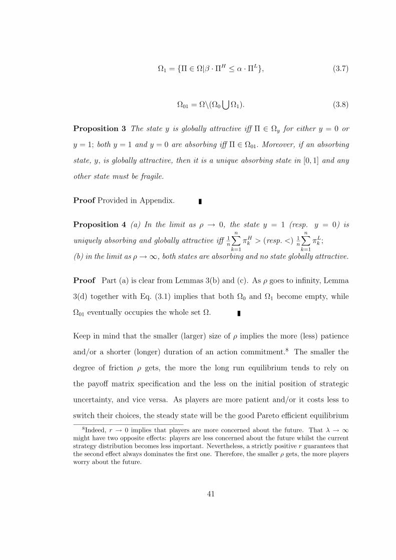
Ω1 = Π ∈ Ω|β · ΠH ≤ α · ΠL, (3.7)

Ω01 = Ω\(Ω0

⋃Ω1). (3.8)

Proposition 3 The state y is globally attractive iff Π ∈ Ωy for either y = 0 or

y = 1; both y = 1 and y = 0 are absorbing iff Π ∈ Ω01. Moreover, if an absorbing

state, y, is globally attractive, then it is a unique absorbing state in [0, 1] and any

other state must be fragile.

Proof Provided in Appendix.

Proposition 4 (a) In the limit as ρ → 0, the state y = 1 (resp. y = 0) is

uniquely absorbing and globally attractive iff 1n

n∑k=1

πHk > (resp. <) 1

n

n∑k=1

πLk ;

(b) in the limit as ρ →∞, both states are absorbing and no state globally attractive.

Proof Part (a) is clear from Lemmas 3(b) and (c). As ρ goes to infinity, Lemma

3(d) together with Eq. (3.1) implies that both Ω0 and Ω1 become empty, while

Ω01 eventually occupies the whole set Ω.

Keep in mind that the smaller (larger) size of ρ implies the more (less) patience

and/or a shorter (longer) duration of an action commitment.8 The smaller the

degree of friction ρ gets, the more the long run equilibrium tends to rely on

the payoff matrix specification and the less on the initial position of strategic

uncertainty, and vice versa. As players are more patient and/or it costs less to

switch their choices, the steady state will be the good Pareto efficient equilibrium

8Indeed, r → 0 implies that players are more concerned about the future. That λ → ∞might have two opposite effects: players are less concerned about the future whilst the currentstrategy distribution becomes less important. Nevertheless, a strictly positive r guarantees thatthe second effect always dominates the first one. Therefore, the smaller ρ gets, the more playersworry about the future.

41

as long as the “static” unweighted average from H exceeds that from taking L.

The interpretation is as follows: Suppose you are going to play a one shot game

G(n, Π). Since you are confronted with (n − 1) opponents, there are n possible

events, denoted Ak−1, k = 1, 2, ..., n, where exactly (k−1) opponents choose action

H. You assume that each of those events takes place with equal probability 1n, and

makes your best response. Notice that this necessarily implies some correlation

among your opponents’ choices.

On the other extreme case of ρ approaching to infinity, sometimes called best

response dynamics, both states may obtain in the long run and exactly which

one would come out depends solely upon what the initial state was. In fact,

Matsui [1992] verifies an equivalence between the best response dynamics and a

static equilibrium concept attributed to Swinkels [1992a]. This notion, called an

evolutionary stability with equilibrium entrants, imposes an additional restriction

on the qualification of mutants, thus is weaker than the traditional evolutionary

stability. Notice that the connection9 of “myopic” replicator dynamics to strate-

gic stability or rationalizability would be vacuous in coordination games, because

both Nash equilibria simply survive the strict iterated admissibility. Such inde-

terminacy is resolved if we perturb the dynamical system with a constant flow

of mutations and experimentations. Kim [1992b] not only characterizes the long

run ergodic equilibrium of the resulting stochastic dynamics in the limit as the

probability of mutations approaches to zero, but also provides clear and intuitive

comparions between the equilibrium selections derived. The reader is urged to

refer to that paper for details.

9Refer to Swinkels [1992b] and references therein.

42

3.5 Equivalence with Global Perturbation

The global perturbation approach of Carlsson and Van Damme [1990, 1991] is

based on the idea that players are uncertain not only about the payoffs but also

their modeling of the game itself. Each player i will receive a private signal θi that

provides an unbiased estimate of θ, but the signals are noisy so the true value of

θ is not common knowledge. Let Θ be a random variable and let Eini=1 be an n

tuple of i.i.d. random variables, each having zero mean. The Ei are independent

of Θ, with a continuous density and a support within [−1, 1]. For ε > 0, write

Θεi = Θ + εEi.

Notice that ε measures perfectness of the common knowledge.

Given this structure, we formally define the incomplete information game

Gε(n, Π) described by the following rules: A realization (θ, θ1, ..., θn) of (Θ, Θε1, ..., Θ

εn)

is drawn, player i is informed only about θi and chooses between H and L, each

player i receives payoffs as determined by G(n, Π(θ)) and the action taken. Even

if player i knows upon having observed θi that the true θ lies in [θi − ε, θi + ε]

and that all other θj’s in [θi − 2ε, θi + 2ε], this fact is not common knowledge.

Now suppose that θj is realized as, say, θi − 2ε, then player j knows that θ lies in

[θj−ε, θj +ε], thus in [θi−3ε, θi +ε], and that θi must be in [θj−2ε, θj +2ε], thus

in [θi − 4ε, θi]. The problem is that player i does not know that player j knows

that θi lies in [θi− 4ε, θi]. This argument applies also to all the other less extreme

realizations of θj. Lack of common knowledge expands all the way down, and

thus enables remote areas of dominated strategies (−∞, θ) and (θ,∞) to exert an

influence, however tiny ε might be as far as it is strictly positive.10

We confine our attention to the perturbation pHk (resp. pL

n−k) that satisfies the

10Such remote areas play an important role in Rubinstein [1989] as well.

43

following two conditions:

Assumption 1 (a) They are continuous, monotonically increasing (resp. de-

creasing) in θ, and unbounded above and below, ∀k; (b) the original unperturbed

game obtains with θ = 0, i.e. pζ· (0) = πζ

· for ζ =H,L.

Let θ (resp. θ) the infimum (resp. supremum) of θ’s such that H (resp. L) is a

strictly dominant strategy in a game with payoff realization θ. By assumption 1

above, it is obvious that −∞ < θ < 0 < θ < +∞.

Assumption 2 The Θ is uniformly distributed over an interval ⊃ [θ, θ].

One might ask whether this is a big perturbation. Answer is both no and yes. As it

turns out, our goal is to see what happens at the exactly original games in the limit

as the common knowledge about payoffs is almost perfect, after characterizing

the equilibrium behavior assuming this perturbation. Neverthless, players are

taking very different situations from the original game into account through his

contemplation process. Uniformity part would play an important role, since only

order but not location of the realizations of random noise variable matters. We

believe that our main points would still emerge without this restriction, but we

have not verified that this is the case. A guess on the relaxation of this assumption

will be made in the last section.

Under these assumptions, an iterative elimination of strictly dominated strate-

gies, namely strict iterated admissibility, will be applied. The next lemma shows

that the Bayesian Nash equilibrium has the cutoff property, and that the game

considered here is indeed dominance solvable.

Lemma 4 If Assumption 1 and 2 hold, then the equilibrium is characterized by

cutoff θGP such that player i optimally chooses H (resp. L) iff θi > (resp. <)θGP .

Furthermore, θGP is a unique root of the equation 1n

∑k pH

k (θ) = 1n

∑k pL

k (θ).

44

Proof Provided in Appendix.

Recall that the perturbed game will correspond to the original unperturbed

game when θ = 0. We are interested in what happens at θ = 0 in the limit as

the common knowledge about payoffs becomes arbitrarily perfect, i.e. ε goes to

zero. Recall that |θi| < ε if θ = 0. So if θGP > (resp. <)0 for ε small enough then

θi < (resp. >)θGP for all i when θ = 0. In other words, if θGP < (resp. >)0, then

when θ = 0 and ε is sufficiently small, the results of iterative strict dominance

prescribe that all players play H (resp. L). So we say that the equilibrium H in

the unperturbed game is robust with respect to global perturbation if θGP < 0, and

that L is robust if θGP > 0. Recall that the state y be the fraction of population

taking action H. Then argument thus far yields:

Main Theorem The y = 1 (resp. 0) is the unique absorbing and globally

attractive state in the limit as ρ → 0 if and only if action H (resp. L) is robust

with respect to global perturbation.

A couple of papers in the literature deserve some mention. Harsanyi [1973]

uses a similar perturbation to justify mixed strategy equilibria. His formulation

requires, however, that the value of θ be common knowledge so observing θi implies

knowing the realization of Ei, but not E−i’s, and that the payoff of player i

depends on θi rather than on θ. Fudenberg, Kreps, and Levine [1988] argues that

an equilibrium that is unreasonable (in the sense of being eliminated by Nash

refinements) in a given game may not be unreasonable in nearby games. They

assert that every strict equilibrium is reasonable and they roughly show that

every normal form perfect equilibrium can be approximated by strict equilibria

of nearby games, hence, that any such equilibrium is reasonable as well. Their

paper differs from global perturbation in the definition of nearness of games and

45

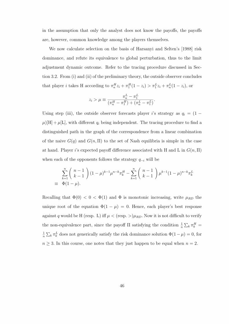
in the assumption that only the analyst does not know the payoffs, the payoffs

are, however, common knowledge among the players themselves.

We now calculate selection on the basis of Harsanyi and Selten’s [1988] risk

dominance, and refute its equivalence to global perturbation, thus to the limit

adjustment dynamic outcome. Refer to the tracing procedure discussed in Sec-

tion 3.2. From (i) and (ii) of the preliminary theory, the outside observer concludes

that player i takes H according to πHn zi + πH

1 (1− zi) > πL1 zi + πL

n (1− zi), or

zi > µ ≡ πLn − πL

1

(πHn − πH

1 ) + (πLn − πL

1 ).

Using step (iii), the outside observer forecasts player i’s strategy as qi = (1 −

µ)[H] + µ[L], with different qi being independent. The tracing procedure to find a

distinguished path in the graph of the correspondence from a linear combination

of the naive G(q) and G(n, Π) to the set of Nash equilibria is simple in the case

at hand. Player i’s expected payoff difference associated with H and L in G(n, Π)

when each of the opponents follows the strategy q−i will be

n∑k=1

(n− 1k − 1

)(1− µ)k−1µn−kπH

k −n∑

k=1

(n− 1k − 1

)µk−1(1− µ)n−kπL

k

≡ Φ(1− µ).

Recalling that Φ(0) < 0 < Φ(1) and Φ is monotonic increasing, write µRD the

unique root of the equation Φ(1 − µ) = 0. Hence, each player’s best response

against q would be H (resp. L) iff µ < (resp. >)µRD. Now it is not difficult to verify

the non-equivalence part, since the payoff Π satisfying the condition 1n

∑k πH

k =

1n

∑k πL

k does not generically satisfy the risk dominance solution Φ(1−µ) = 0, for

n ≥ 3. In this course, one notes that they just happen to be equal when n = 2.

46

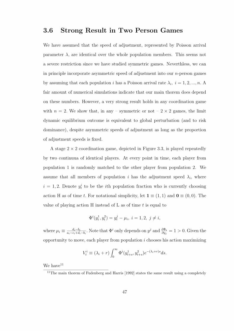
3.6 Strong Result in Two Person Games

We have assumed that the speed of adjustment, represented by Poisson arrival

parameter λ, are identical over the whole population members. This seems not

a severe restriction since we have studied symmetric games. Neverthless, we can

in principle incorporate asymmetric speed of adjustment into our n-person games

by assuming that each population i has a Poisson arrival rate λi, i = 1, 2, ..., n. A

fair amount of numerical simulations indicate that our main thorem does depend

on these numbers. However, a very strong result holds in any coordination game

with n = 2. We show that, in any – symmetric or not – 2 × 2 games, the limit

dynamic equilibrium outcome is equivalent to global perturbation (and to risk

dominance), despite asymmetric speeds of adjustment as long as the proportion

of adjustment speeds is fixed.

A stage 2× 2 coordination game, depicted in Figure 3.3, is played repeatedly

by two continuua of identical players. At every point in time, each player from

population 1 is randomly matched to the other player from population 2. We

assume that all members of population i has the adjustment speed λi, where

i = 1, 2. Denote yit to be the ith population fraction who is currently choosing

action H as of time t. For notational simplicity, let 1 ≡ (1, 1) and 0 ≡ (0, 0). The

value of playing action H instead of L as of time t is equal to

Φi(y1t , y

2t ) = yj

t − µi, i = 1, 2, j 6= i,

where µi ≡ di−bi

ai−ci+di−bi. Note that Φi only depends on yj and ∂Φi

∂yj= 1 > 0. Given the

opportunity to move, each player from population i chooses his action maximizing

V it ≡ (λi + r)

∫ ∞

0Φi(y1

t+s, y2t+s)e

−(λi+r)sds.

We have11

11The main thorem of Fudenberg and Harris [1992] states the same result using a completely

47

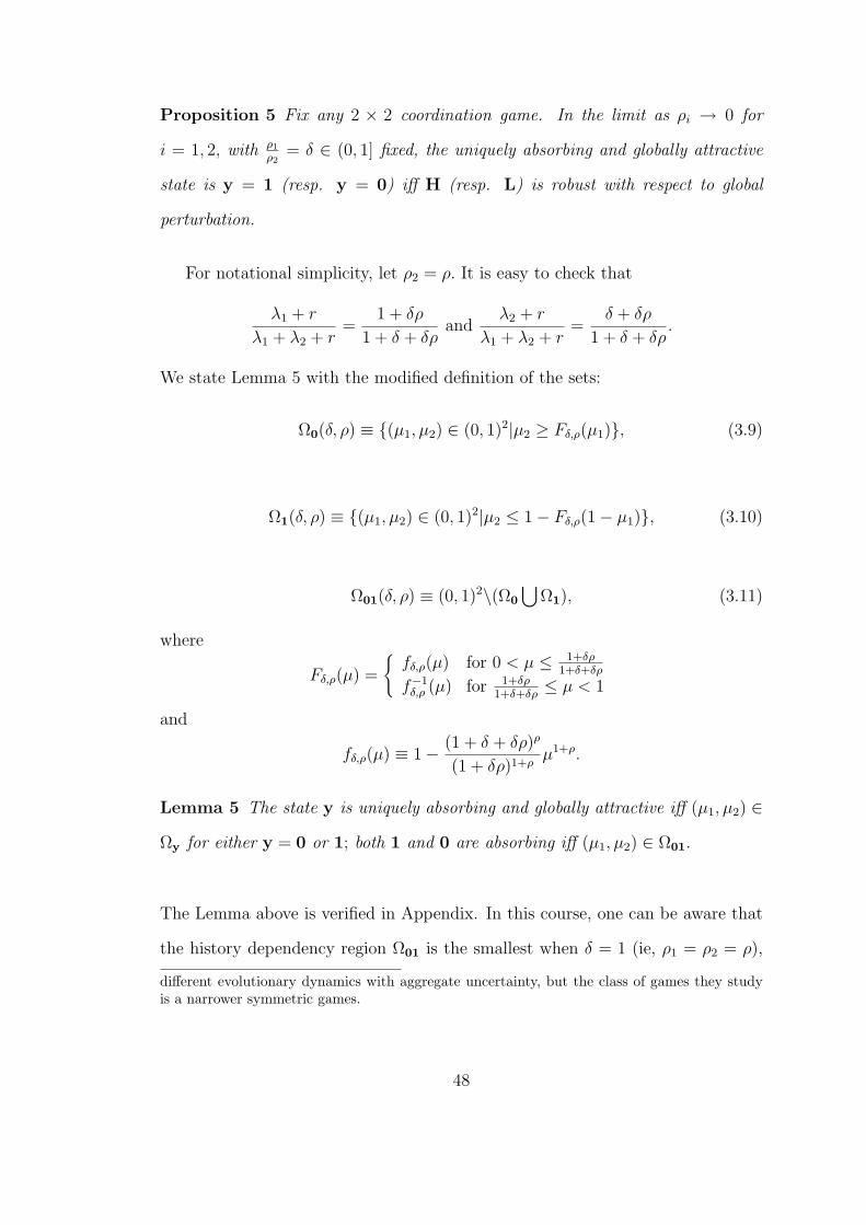
Proposition 5 Fix any 2 × 2 coordination game. In the limit as ρi → 0 for

i = 1, 2, with ρ1

ρ2= δ ∈ (0, 1] fixed, the uniquely absorbing and globally attractive

state is y = 1 (resp. y = 0) iff H (resp. L) is robust with respect to global

perturbation.

For notational simplicity, let ρ2 = ρ. It is easy to check that

λ1 + r

λ1 + λ2 + r=

1 + δρ

1 + δ + δρand

λ2 + r

λ1 + λ2 + r=

δ + δρ

1 + δ + δρ.

We state Lemma 5 with the modified definition of the sets:

Ω0(δ, ρ) ≡ (µ1, µ2) ∈ (0, 1)2|µ2 ≥ Fδ,ρ(µ1), (3.9)

Ω1(δ, ρ) ≡ (µ1, µ2) ∈ (0, 1)2|µ2 ≤ 1− Fδ,ρ(1− µ1), (3.10)

Ω01(δ, ρ) ≡ (0, 1)2\(Ω0

⋃Ω1), (3.11)

where

Fδ,ρ(µ) =

fδ,ρ(µ) for 0 < µ ≤ 1+δρ

1+δ+δρ

f−1δ,ρ (µ) for 1+δρ

1+δ+δρ≤ µ < 1

and

fδ,ρ(µ) ≡ 1− (1 + δ + δρ)ρ

(1 + δρ)1+ρµ1+ρ.

Lemma 5 The state y is uniquely absorbing and globally attractive iff (µ1, µ2) ∈

Ωy for either y = 0 or 1; both 1 and 0 are absorbing iff (µ1, µ2) ∈ Ω01.

The Lemma above is verified in Appendix. In this course, one can be aware that

the history dependency region Ω01 is the smallest when δ = 1 (ie, ρ1 = ρ2 = ρ),

different evolutionary dynamics with aggregate uncertainty, but the class of games they studyis a narrower symmetric games.

48

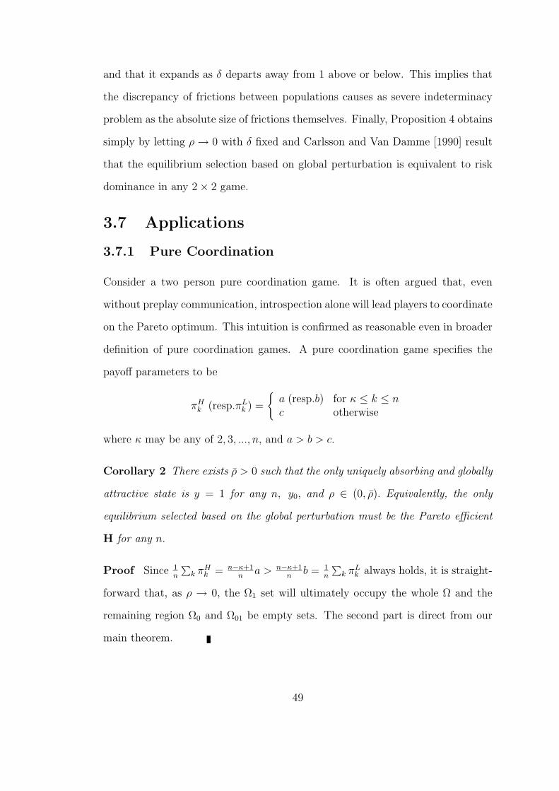
and that it expands as δ departs away from 1 above or below. This implies that

the discrepancy of frictions between populations causes as severe indeterminacy

problem as the absolute size of frictions themselves. Finally, Proposition 4 obtains

simply by letting ρ → 0 with δ fixed and Carlsson and Van Damme [1990] result

that the equilibrium selection based on global perturbation is equivalent to risk

dominance in any 2× 2 game.

3.7 Applications

3.7.1 Pure Coordination

Consider a two person pure coordination game. It is often argued that, even

without preplay communication, introspection alone will lead players to coordinate

on the Pareto optimum. This intuition is confirmed as reasonable even in broader

definition of pure coordination games. A pure coordination game specifies the

payoff parameters to be

πHk (resp.πL

k ) =

a (resp.b) for κ ≤ k ≤ nc otherwise

where κ may be any of 2, 3, ..., n, and a > b > c.

Corollary 2 There exists ρ > 0 such that the only uniquely absorbing and globally

attractive state is y = 1 for any n, y0, and ρ ∈ (0, ρ). Equivalently, the only

equilibrium selected based on the global perturbation must be the Pareto efficient

H for any n.

Proof Since 1n

∑k πH

k = n−κ+1n

a > n−κ+1n

b = 1n

∑k πL

k always holds, it is straight-

forward that, as ρ → 0, the Ω1 set will ultimately occupy the whole Ω and the

remaining region Ω0 and Ω01 be empty sets. The second part is direct from our

main theorem.

49

3.7.2 Stag Hunt

The most general payoff specification that includes the game discussed in the

expository section is as follows:

πLk = x ∈ (0, 1) all k

0 = πH1 ≤ πH

2 ≤ ... ≤ πHn = 1.

Besides its practical applicability, this game has a couple of merits to analyze.

First, the Pareto optimality is at odds with the security, so which outcome would

actually appear may be controversial. Second, it reduces the Ω sets to a one

dimensional space, which makes the results extremely intuitive and facilitates

numerical studies. Recalling that · denotes a dot product of two vectors, we

define

u(n, ρ) ≡ α · ΠH and `(n, ρ) ≡ β · ΠH (3.12)

where αk’s and βk’s are as in Eq. (3.5). Directly applying proposition 1 and 2

yields:

Lemma 6 (a) The state y = 1 is globally attractive iff x ≥ u(n, ρ); y = 0 is

globally attractive iff x ≤ `(n, ρ); both y = 1 and y = 0 are absorbing iff `(n, ρ) ≤

x ≤ u(n, ρ);

(b) in the limit as ρ → 0, the state y = 1 (resp. y = 0) is globally attractive iff

x < (resp. >) 1n

∑k

πHk ≡ xLD; (c) in the limit as ρ →∞, both states are absorbing.

Corollary 3

xLD =1

n

n∑k=1

πHk = xGP 6= xRD

The LD in the subscript stands for ‘limit dynamic’. Corollary 3 immediately

follows from Lemma 6 and Carlsson and Van Damme [1991].

50

3.8 Experimental Implications

A brief survey of Van Huyck et al. [1990, 1991] experimental results is offered.

Each treatment typically lasts ten stages but the number of stages was not an-

nounced in advance in some experiments. A summary statistic of subjects’ strat-

egy choices was publicly announced after each stage. At the end of each experi-

ment, subjects were paid the sum of their payoffs in the games they played. In

each of the games, each player i chooses a pure strategy, denoted ei and called

effort, from the set 1, ..., 7. In each stage, each player’s payoff was determined

by his own effort and a simple summary statistics of those of the players in his

group. This statistic was either minimum or median of group effort choices. The

parameter values were given for these normal forms12 to be of coordination games

with seven strict Pareto ranked symmetric pure strategy Nash equilibria. In every

game, the payoff dominance selects all players’ choosing the highest effort, i.e. 7,

irrespective of the number of subjects in a group. With respect to group size, a

large group consists of 14 to 16 players whilst a small group of only two persons.

Despite payoff dominance, in large group minimum treatments subjects ini-

tially choose widely dispersed efforts and then rapidly approached the lowest ef-

fort, e = 1 : up to 84% of the subjects reached that effort within a few stages. In

one treatment in which the parameters were adjusted so as for the highest effort

e = 7 to be weakly dominant, approximately 96 percentage reached that effort by

the fifth stage. This result may justify our maintained assumption that no strictly

dominated strategy will be played at all.13 In small group experiments, subjects’

initial choices varied substantially and then drifted over time with no clearly

12Van Huyck et al.1990 article for minimum treatments and 1991 research for median onescontain parameter values actually used in the experiments and the resulting normal forms.

13No conflict arises with Cooper et al. [1990] experimental evidence, which just asserts thatany addition or deletion of dominated strategies may affect the equilibrium actually selected.

51

discernable trend. By contrast, subjects in every median treatment converged

completely and promptly to the Nash equilibrium determined by the “historical

accident” of their initial stage median, despite considerable variation in the initial

median across treatments. In brevity, it exhibits a strong history dependency.

Finally, in large group median experiments with pure coordination game, players

move swiftly to the Pareto best equilibrium action. This last observation can

be at least partially explained by our corollary 2 and the fact that subjets were

allowed to switch their choices every period.

Our simple model captures many salient features that were reported above.

To see this, we consider a stag hunt game as follows:

πHk =

1 if κ ≤ k ≤ n0 otherwise,

where κ denotes the minimum number of players necessary for a successful stag

hunt. Note that the minimum rule specifies κ = n and that the median vote does

κ = n+12

. Plugging into Eq. (3.12) gives rise to

u =n∑

k=κ

αk and ` =n∑

k=κ

βk,

with αk and βk as defined in Eq. (3.5). Remember from lemma 6 that the steady

state could be H and L regardless of the initial state, respectively, according as

x < ` and x > u. Certainly there might exist an equilibrium path converging

to, say, H when x > u, if the initial population fraction of stag hunters is very

high. However, we execute the numerical analysis as if the globally attractive

state was globally stable. This is silly but can be tolerated reflecting the fact that

the two regions of global attraction roughly offset each other. In the case where

x ∈ [`, u], exactly which equilibrium will be obtained in the long run hinges on

y0, the historical accident of initial states. For the sake of calculation, we impose

the monotonicity requirement, that is, only the paths monotonically converging to

52

either H and L will be taken into account. That is, any cyclical path is ruled out.

Deterministic nature of the present dynamic together with monotonicity imply

the existence of a unique critical value of x, below which the path converges to

H, and vice-versa.

We assume throughout that x is uniformly distributed over [0, 1]. Two remarks

are in order. First, the strategic uncertainty as has been understood should im-

ply the distribution over the initial y0 with x being fixed. It causes numerically

little problem to consider y0 as deterministic and instead x as uncertain. An-

other justification might be the uncertainty on the part of the experimenter about

subjects’ subjective evaluations of the fixed monetary compensation x. Second,

relaxing reasonably the uniformity of the x-distribution here only seems to make

our result stronger. As in Van Huyck et al.’s experiments, we let n = 2 for a small

group and n = 15 for a large group.

Let y(x) denote the inverse function of

n∑k=κ

(n− 1k − 1

)yk−1(1− y)n−k = x,

where the left (resp. right) hand side is the expected payoff from H (resp. L).

Deterministic nature of the model and the monotonicity of paths make it clear that

a player should choose action H (resp. L) if y0 > (resp. <)y(x) in the intermediate

history dependency region, given an opportunity to switch. The probability that

the steady state be the Pareto inferior Nash L will be at least approximately:

Pr(L is the steady state) = Pr(x ≥ u) + Pr(` < x < u, y0 < y(x))

= (1− u) +∫ u

`y(x)dx,

where u and ` are calculated using Eq. (3.5).

In small group treatment, the probability that the steady state is L would

be (1 − 1+ρ2+ρ

) +∫ u` xdx = 0.5 regardless of ρ. Under a large group minimum rule,

53

this probability will be expressed as (1−u)+∫ u` x

114 dx. Table 3.2 provides several

simulations according to varying parameters.14 The range of x in which the Pareto

inferior equilibrium L could be selected irrespective of the initial states is very

broad, unless subjects are extremely impatient. On the other hand, with a big

ρ value, the portion of which both strict equilibria are absorbing is large. But

even in such a situation, the basin of attraction with respect to initial strategic

uncertainty is much larger for L than that for H under maintained assumption

of the path monotonicty. These are reflected on the fact that the steady state

is likely to settle down on the inferior equilibrium L with probability of at least

93.3 percent and up to 97 percent. The high probability of attaining the Pareto

inferior equilibrium is consistent with coordination failures which were observed

in Van Huyck et al’s experimental results.

Table 3.3 analogously analyzes the large group median treatments. The prob-

ability that the Pareto inferior Nash equilibrium L will be selected as the long run

state is shown to be stable around 46 percent. The point here is that, for each ρ

given, a relatively wide range between ` and u indicates a strong dependence on

the initial state, or put differently, “historical accident.” For instance with ρ = 1,

the history dependence region [.008, .125] of a minimum rule is in sharp contrast

to [.300, .767] of median vote. Comparison of tables show that this characteristic

is fairly robust to the somewhat arbitrary parameter ρ size.

We close the section with some loose comments on Harrison and Hirshleifer’s

[1989] public goods provision experiments. Consider two popular models, the

“weakest link” and the “best shot.” The weakest link model refers to the situa-

tion where failure of even a single person brings about miserable ruins to all, for

example military units defending segments of the front against an enemy offen-

14 All simulations were carried out using Mathematica.

54

sive. In contrast, the best shot refers to the case where only one’s provision or

success is enough for all, such as rats trying to bell the cat. HH convincingly ar-

gues that the “free-rider” problem would be less (more) serious, thus cooperation

would be more (less) likely to obtain, in the weakest link (best shot, respectively)

model. Reflecting the fact that the weakest link is strategically equivalent to the

stag hunt game under the minimum rule, their insight and the basic theme here

seemingly contradict each other. This is not the case. Take the example of mili-

tary units defending segments of the front against an enemy offensive. If all other

units are successfully defending their own segments and if this fact is common

knowledge then it certainly would be in my interest to defend my own. How-

ever, once even a single segment is broken through, running away will be everyone

else’s best response. How does one know the others are doing well? As an obvi-

ous guess, it seems likely that some means of signalling, such as cheap talk and

sequential move structure, could enhance the possibility of cooperation. On the

contrary, the actual failure of or little doubt about the perfect defense will make

the good equilibrium collapse.15 We view this as an underlying reason for HH’s

experimental outcomes, in which subjects show a substantial cooperation with

the sequential protocol while little clearcut evidence on cooperation or behavioral

pattern is perceived with the sealed bid protocol.

3.9 Concluding Remarks

The present paper has of course some shortcomings, especially in its critical de-

pendence on a somewhat arbitrary parameter ρ, the effective discount rate or

friction. Uniformity of the distribution of random noise variables looks to be also

restrictive, although a scrutiny of the proofs in Carlsson and Van Damme [1990]

15 It is a contagious equilibrium in Kandori’s [1992] sense.

55

might suggest a relaxation of this assumption. Our conjecture is as follows: under

a general distribution with compact support and given ε > 0, there exists η(ε) > 0

satisfying limε→0 η = 0 such that player i optimally chooses action H (resp. L) if

his private signal θi > θGP +η (resp. < θGP −η). Moreover, this almost dominance

solvability in the limit is reduced to exact dominance solvability under uniform

distribution.

Effort is needed to generalize in encompassing multi actions and/or asymmetric

payoffs. Technical difficuties arise from the large amount of case distinctions and

calculations. With m actions, we have to consider 2m−1 number of Ω(·) sets, where

only a is globally attractive if Π ∈ Ωa and only a1, a2, ..., ai are absorbing if

Π ∈ Ωa1a2...aifor 2 ≤ i ≤ m. Payoff asymmety in n person m action games require

considering an nm dimensional space. While there is, at least in principle, no

reason why adjustment dynamics or global perturbation fails to be well-defined

in the general setting, it is known that risk dominance may well be troublesome

because of intransitivities between strict equilibria. In view of our corollary 2,

this line of research seems to include as a special example the former part of

Kandori and Rob [1992], which abandons risk dominance even in a two person

m-action coordination game. Experimental results along the lines of Harrison and

Hirshleifer [1989], Cooper et al. [1992], and Matsui [1991] suggest that it is worth

exploring the introduction of a cheap talk argument, thus to see whether and

how the possibility of cooperation could be enhanced through a costless preplay

communication with more than two players.

56

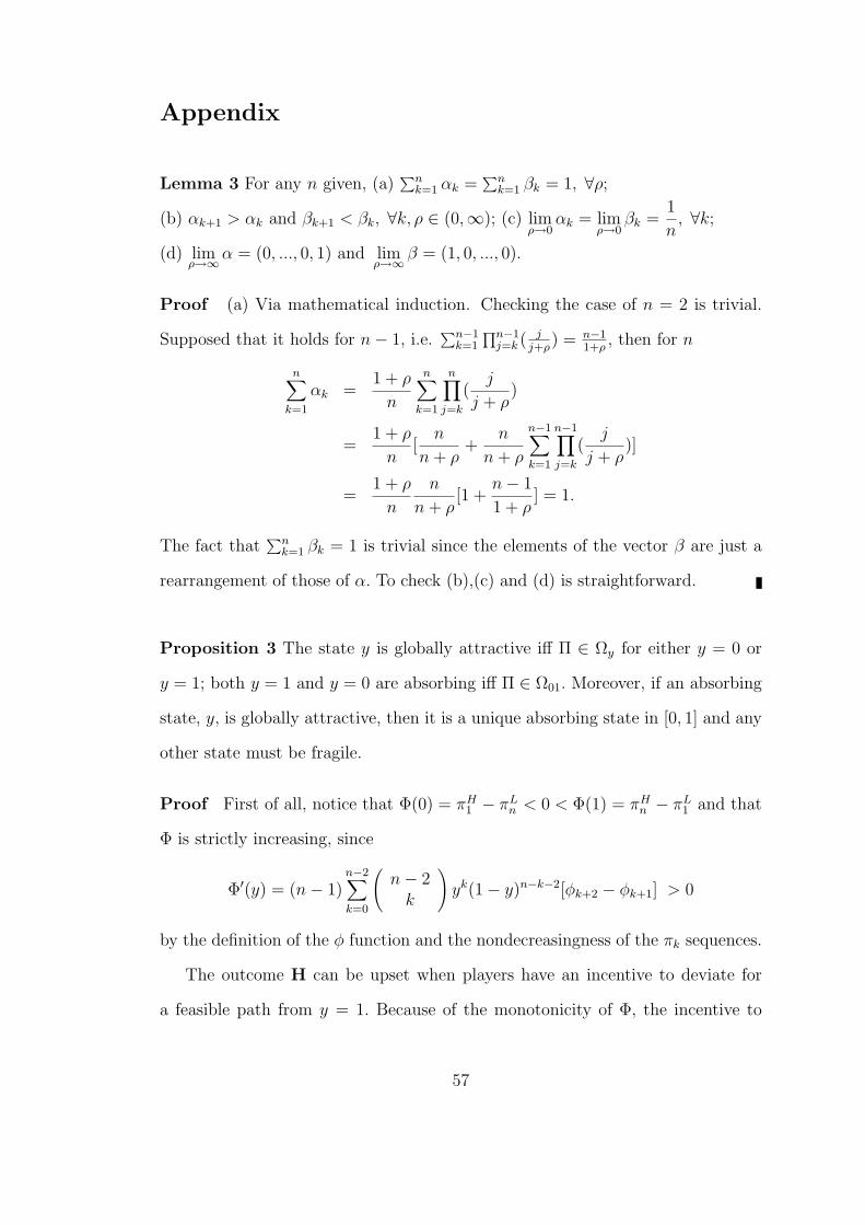
Appendix

Lemma 3 For any n given, (a)∑n

k=1 αk =∑n

k=1 βk = 1, ∀ρ;

(b) αk+1 > αk and βk+1 < βk, ∀k, ρ ∈ (0,∞); (c) limρ→0

αk = limρ→0

βk =1

n, ∀k;

(d) limρ→∞

α = (0, ..., 0, 1) and limρ→∞

β = (1, 0, ..., 0).

Proof (a) Via mathematical induction. Checking the case of n = 2 is trivial.

Supposed that it holds for n− 1, i.e.∑n−1

k=1

∏n−1j=k ( j

j+ρ) = n−1

1+ρ, then for n

n∑k=1

αk =1 + ρ

n

n∑k=1

n∏j=k

(j

j + ρ)

=1 + ρ

n[

n

n + ρ+

n

n + ρ

n−1∑k=1

n−1∏j=k

(j

j + ρ)]

=1 + ρ

n

n

n + ρ[1 +

n− 1

1 + ρ] = 1.

The fact that∑n

k=1 βk = 1 is trivial since the elements of the vector β are just a

rearrangement of those of α. To check (b),(c) and (d) is straightforward.

Proposition 3 The state y is globally attractive iff Π ∈ Ωy for either y = 0 or

y = 1; both y = 1 and y = 0 are absorbing iff Π ∈ Ω01. Moreover, if an absorbing

state, y, is globally attractive, then it is a unique absorbing state in [0, 1] and any

other state must be fragile.

Proof First of all, notice that Φ(0) = πH1 − πL

n < 0 < Φ(1) = πHn − πL

1 and that

Φ is strictly increasing, since

Φ′(y) = (n− 1)n−2∑k=0

(n− 2

k

)yk(1− y)n−k−2[φk+2 − φk+1] > 0

by the definition of the φ function and the nondecreasingness of the πk sequences.

The outcome H can be upset when players have an incentive to deviate for

a feasible path from y = 1. Because of the monotonicity of Φ, the incentive to

57

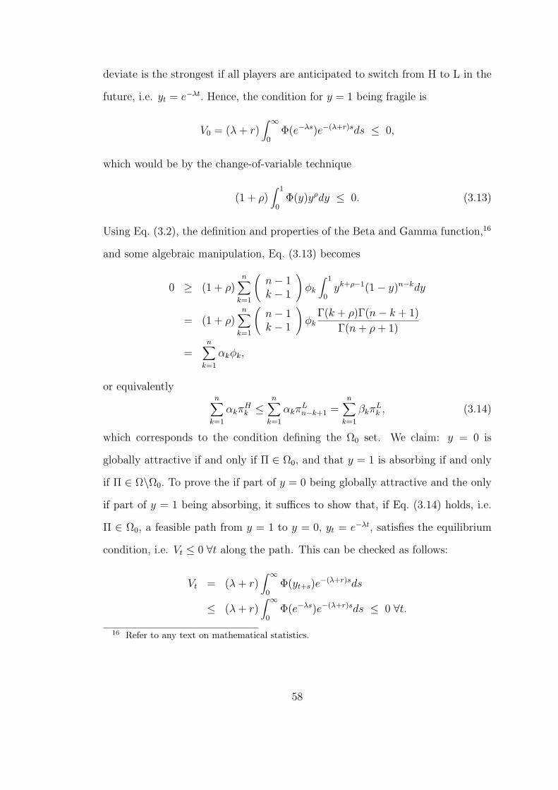
deviate is the strongest if all players are anticipated to switch from H to L in the

future, i.e. yt = e−λt. Hence, the condition for y = 1 being fragile is

V0 = (λ + r)∫ ∞

0Φ(e−λs)e−(λ+r)sds ≤ 0,

which would be by the change-of-variable technique

(1 + ρ)∫ 1

0Φ(y)yρdy ≤ 0. (3.13)

Using Eq. (3.2), the definition and properties of the Beta and Gamma function,16

and some algebraic manipulation, Eq. (3.13) becomes

0 ≥ (1 + ρ)n∑

k=1

(n− 1k − 1

)φk

∫ 1

0yk+ρ−1(1− y)n−kdy

= (1 + ρ)n∑

k=1

(n− 1k − 1

)φk

Γ(k + ρ)Γ(n− k + 1)

Γ(n + ρ + 1)

=n∑

k=1

αkφk,

or equivalentlyn∑

k=1

αkπHk ≤

n∑k=1

αkπLn−k+1 =

n∑k=1

βkπLk , (3.14)

which corresponds to the condition defining the Ω0 set. We claim: y = 0 is

globally attractive if and only if Π ∈ Ω0, and that y = 1 is absorbing if and only

if Π ∈ Ω\Ω0. To prove the if part of y = 0 being globally attractive and the only

if part of y = 1 being absorbing, it suffices to show that, if Eq. (3.14) holds, i.e.

Π ∈ Ω0, a feasible path from y = 1 to y = 0, yt = e−λt, satisfies the equilibrium

condition, i.e. Vt ≤ 0 ∀t along the path. This can be checked as follows:

Vt = (λ + r)∫ ∞

0Φ(yt+s)e

−(λ+r)sds

≤ (λ + r)∫ ∞

0Φ(e−λs)e−(λ+r)sds ≤ 0 ∀t.

16 Refer to any text on mathematical statistics.

58

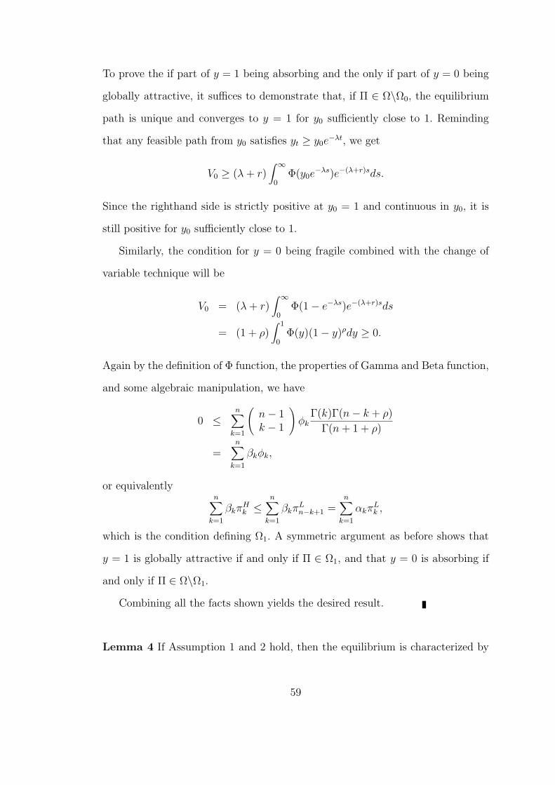
To prove the if part of y = 1 being absorbing and the only if part of y = 0 being

globally attractive, it suffices to demonstrate that, if Π ∈ Ω\Ω0, the equilibrium

path is unique and converges to y = 1 for y0 sufficiently close to 1. Reminding

that any feasible path from y0 satisfies yt ≥ y0e−λt, we get

V0 ≥ (λ + r)∫ ∞

0Φ(y0e

−λs)e−(λ+r)sds.

Since the righthand side is strictly positive at y0 = 1 and continuous in y0, it is

still positive for y0 sufficiently close to 1.

Similarly, the condition for y = 0 being fragile combined with the change of

variable technique will be

V0 = (λ + r)∫ ∞

0Φ(1− e−λs)e−(λ+r)sds

= (1 + ρ)∫ 1

0Φ(y)(1− y)ρdy ≥ 0.

Again by the definition of Φ function, the properties of Gamma and Beta function,

and some algebraic manipulation, we have

0 ≤n∑

k=1

(n− 1k − 1

)φk

Γ(k)Γ(n− k + ρ)

Γ(n + 1 + ρ)

=n∑

k=1

βkφk,

or equivalentlyn∑

k=1

βkπHk ≤

n∑k=1

βkπLn−k+1 =

n∑k=1

αkπLk ,

which is the condition defining Ω1. A symmetric argument as before shows that

y = 1 is globally attractive if and only if Π ∈ Ω1, and that y = 0 is absorbing if

and only if Π ∈ Ω\Ω1.

Combining all the facts shown yields the desired result.

Lemma 4 If Assumption 1 and 2 hold, then the equilibrium is characterized by

59

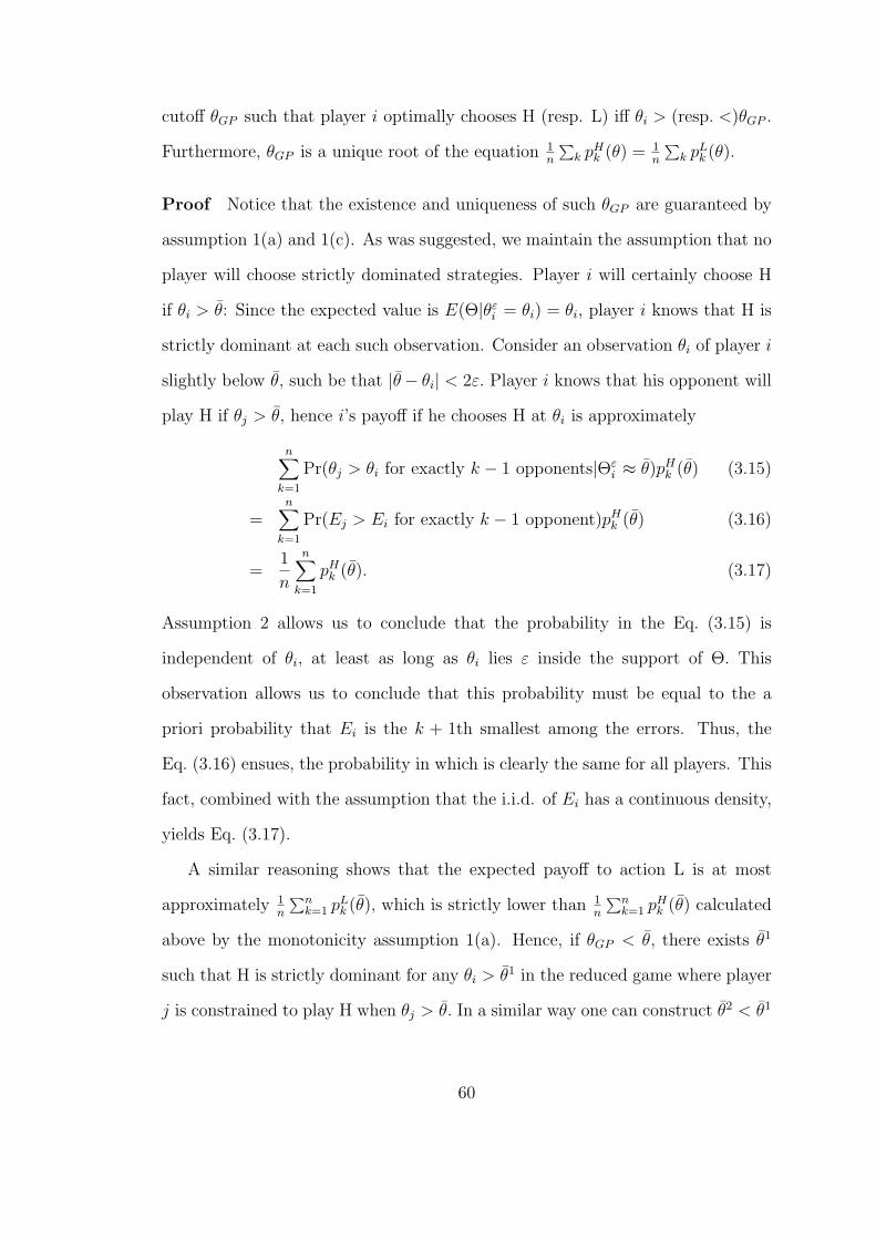
cutoff θGP such that player i optimally chooses H (resp. L) iff θi > (resp. <)θGP .

Furthermore, θGP is a unique root of the equation 1n

∑k pH

k (θ) = 1n

∑k pL

k (θ).

Proof Notice that the existence and uniqueness of such θGP are guaranteed by

assumption 1(a) and 1(c). As was suggested, we maintain the assumption that no

player will choose strictly dominated strategies. Player i will certainly choose H

if θi > θ: Since the expected value is E(Θ|θεi = θi) = θi, player i knows that H is

strictly dominant at each such observation. Consider an observation θi of player i

slightly below θ, such be that |θ− θi| < 2ε. Player i knows that his opponent will

play H if θj > θ, hence i’s payoff if he chooses H at θi is approximately

n∑k=1

Pr(θj > θi for exactly k − 1 opponents|Θεi ≈ θ)pH

k (θ) (3.15)

=n∑

k=1

Pr(Ej > Ei for exactly k − 1 opponent)pHk (θ) (3.16)

=1

n

n∑k=1

pHk (θ). (3.17)

Assumption 2 allows us to conclude that the probability in the Eq. (3.15) is

independent of θi, at least as long as θi lies ε inside the support of Θ. This

observation allows us to conclude that this probability must be equal to the a

priori probability that Ei is the k + 1th smallest among the errors. Thus, the

Eq. (3.16) ensues, the probability in which is clearly the same for all players. This

fact, combined with the assumption that the i.i.d. of Ei has a continuous density,

yields Eq. (3.17).

A similar reasoning shows that the expected payoff to action L is at most

approximately 1n

∑nk=1 pL

k (θ), which is strictly lower than 1n

∑nk=1 pH

k (θ) calculated

above by the monotonicity assumption 1(a). Hence, if θGP < θ, there exists θ1

such that H is strictly dominant for any θi > θ1 in the reduced game where player

j is constrained to play H when θj > θ. In a similar way one can construct θ2 < θ1

60

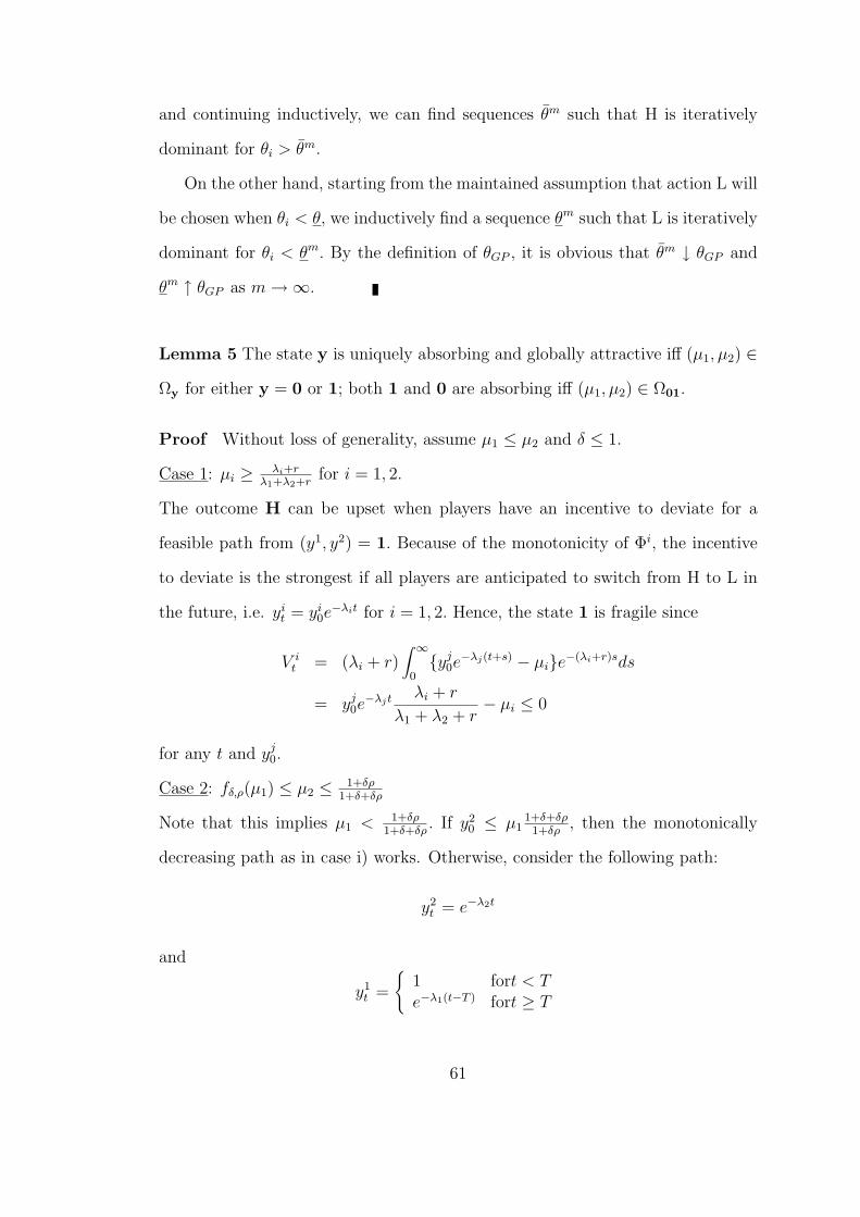
and continuing inductively, we can find sequences θm such that H is iteratively

dominant for θi > θm.

On the other hand, starting from the maintained assumption that action L will

be chosen when θi < θ, we inductively find a sequence θm such that L is iteratively

dominant for θi < θm. By the definition of θGP , it is obvious that θm ↓ θGP and

θm ↑ θGP as m →∞.

Lemma 5 The state y is uniquely absorbing and globally attractive iff (µ1, µ2) ∈

Ωy for either y = 0 or 1; both 1 and 0 are absorbing iff (µ1, µ2) ∈ Ω01.

Proof Without loss of generality, assume µ1 ≤ µ2 and δ ≤ 1.

Case 1: µi ≥ λi+rλ1+λ2+r

for i = 1, 2.

The outcome H can be upset when players have an incentive to deviate for a

feasible path from (y1, y2) = 1. Because of the monotonicity of Φi, the incentive

to deviate is the strongest if all players are anticipated to switch from H to L in

the future, i.e. yit = yi

0e−λit for i = 1, 2. Hence, the state 1 is fragile since

V it = (λi + r)

∫ ∞

0yj

0e−λj(t+s) − µie−(λi+r)sds

= yj0e−λjt λi + r

λ1 + λ2 + r− µi ≤ 0

for any t and yj0.

Case 2: fδ,ρ(µ1) ≤ µ2 ≤ 1+δρ1+δ+δρ

Note that this implies µ1 < 1+δρ1+δ+δρ

. If y20 ≤ µ1

1+δ+δρ1+δρ

, then the monotonically

decreasing path as in case i) works. Otherwise, consider the following path:

y2t = e−λ2t

and

y1t =

1 fort < Te−λ1(t−T ) fort ≥ T

61

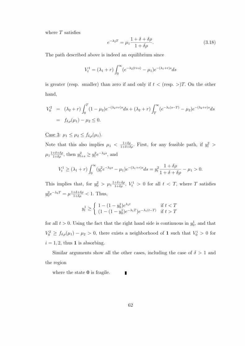
where T satisfies

e−λ2T = µ11 + δ + δρ

1 + δρ. (3.18)

The path described above is indeed an equilibrium since

V 1t = (λ1 + r)

∫ ∞

0(e−λ2(t+s) − µ1)e

−(λ1+r)sds

is greater (resp. smaller) than zero if and only if t < (resp. >)T. On the other

hand,

V 20 = (λ2 + r)

∫ T

0(1− µ2)e

−(λ2+r)sds + (λ2 + r)∫ ∞

T(e−λ1(s−T ) − µ2)e

−(λ2+r)sds

= fδ,ρ(µ1)− µ2 ≤ 0.

Case 3: µ1 ≤ µ2 ≤ fδ,ρ(µ1).

Note that this also implies µ1 < 1+δρ1+δ+δρ

. First, for any feasible path, if y2t >

µ11+δ+δρ1+δρ

, then y2t+s ≥ y2

t e−λ2s, and

V 1t ≥ (λ1 + r)

∫ ∞

0(y2

t e−λ2s − µ1)e

−(λ1+r)sds = y2t

1 + δρ

1 + δ + δρ− µ1 > 0.

This implies that, for y20 > µ1

1+δ+δρ1+δρ

, V 1t > 0 for all t < T, where T satisfies

y20e

−λ2T = µ1+δ+δρ1+δρ

< 1. Thus,

y1t ≥

1− (1− y1

0)eλ1t if t < T

(1− (1− y10)e

−λ1T )e−λ1(t−T ) if t > T

for all t > 0. Using the fact that the right hand side is continuous in y10, and that

V 20 ≥ fδ,ρ(µ1) − µ2 > 0, there exists a neighborhood of 1 such that V i

0 > 0 for

i = 1, 2, thus 1 is absorbing.

Similar arguments show all the other cases, including the case of δ > 1 and

the region

where the state 0 is fragile.

62

Stag HareStag 10, 10 0, xHare x, 0 x, x

Figure 3.1: Two-Player Stag Hunt Game

. Stag Hare Stag HareStag 10,10,10 0,x,0 0,0,x 0,x, xHare x,0,0 x, x,0 x,0,x x, x, x

Stag Hare

Figure 3.2: Three-Player Stag Hunt Game

0 < x < 10

63

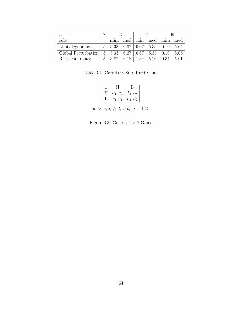
n 2 3 15 99rule mim med min med mim med

Limit Dynamics 5 3.33 6.67 0.67 5.33 0.10 5.05

Global Perturbation 5 3.33 6.67 0.67 5.33 0.10 5.05Risk Dominance 5 3.82 6.18 1.34 5.26 0.34 5.01

Table 3.1: Cutoffs in Stag Hunt Game

.. H LH a1, a2 b1, c2

L c1, b2 d1, d2

ai > ci, ai ≥ di > bi, i = 1, 2.

Figure 3.3: General 2× 2 Game

64

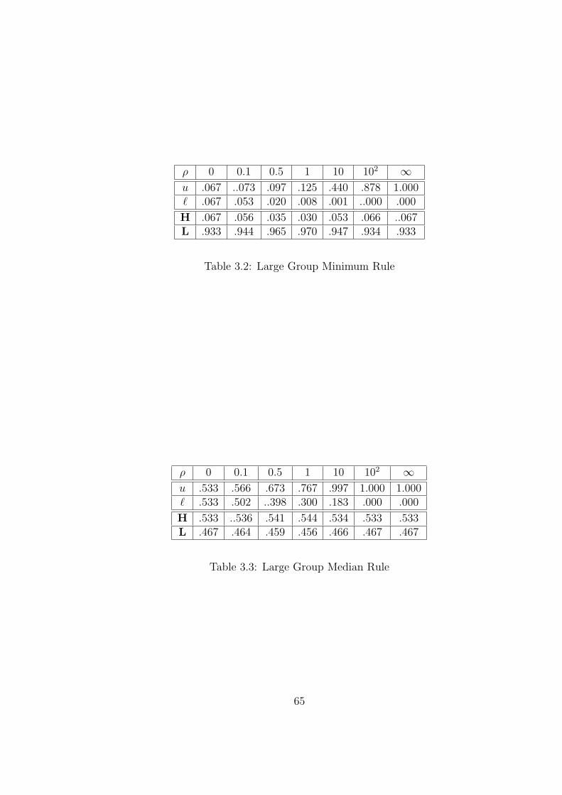
ρ 0 0.1 0.5 1 10 102 ∞u .067 ..073 .097 .125 .440 .878 1.000` .067 .053 .020 .008 .001 ..000 .000

H .067 .056 .035 .030 .053 .066 ..067L .933 .944 .965 .970 .947 .934 .933

Table 3.2: Large Group Minimum Rule

ρ 0 0.1 0.5 1 10 102 ∞u .533 .566 .673 .767 .997 1.000 1.000` .533 .502 ..398 .300 .183 .000 .000

H .533 ..536 .541 .544 .534 .533 .533L .467 .464 .459 .456 .466 .467 .467

Table 3.3: Large Group Median Rule

65

Chapter 4

Evolutionary Learning withExperimentations

66

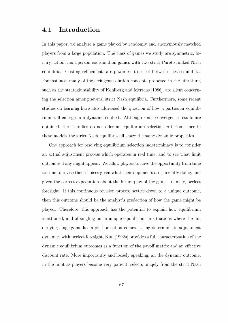
4.1 Introduction

In this paper, we analyze a game played by randomly and anonymously matched

players from a large population. The class of games we study are symmetric, bi-

nary action, multiperson coordination games with two strict Pareto-ranked Nash

equilibria. Existing refinements are powerless to select between these equilibria.

For instance, many of the stringent solution concepts proposed in the literature,

such as the strategic stability of Kohlberg and Mertens [1986], are silent concern-

ing the selection among several strict Nash equilibria. Furthermore, some recent

studies on learning have also addressed the question of how a particular equilib-

rium will emerge in a dynamic context. Although some convergence results are

obtained, these studies do not offer an equilibrium selection criterion, since in

these models the strict Nash equilibria all share the same dynamic properties.

One approach for resolving equilibrium selection indeterminacy is to consider

an actual adjustment process which operates in real time, and to see what limit

outcomes if any might appear. We allow players to have the opportunity from time

to time to revise their choices given what their opponents are currently doing, and

given the correct expectation about the future play of the game—namely, perfect

foresight. If this continuous revision process settles down to a unique outcome,

then this outcome should be the analyst’s predection of how the game might be

played. Therefore, this approach has the potential to explain how equilibrium

is attained, and of singling out a unique equilibrium in situations where the un-

derlying stage game has a plethora of outcomes. Using deterministic adjustment

dynamics with perfect foresight, Kim [1992a] provides a full characterization of the

dynamic equilibrium outcomes as a function of the payoff matrix and an effective

discount rate. More importantly and loosely speaking, an the dynamic outcome,

in the limit as players become very patient, selects uniqely from the strict Nash

67

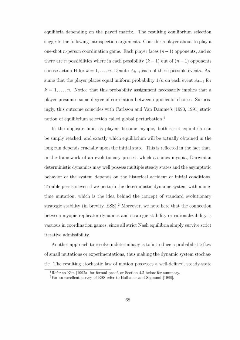
equilibria depending on the payoff matrix. The resulting equilibrium selection

suggests the following introspection arguments. Consider a player about to play a

one-shot n-person coordination game. Each player faces (n−1) opponents, and so

there are n possibilities where in each possibility (k− 1) out of (n− 1) opponents

choose action H for k = 1, . . . , n. Denote Ak−1 each of these possible events. As-

sume that the player places equal uniform probability 1/n on each event Ak−1 for

k = 1, . . . , n. Notice that this probability assignment necessarily implies that a

player presumes some degree of correlation between opponents’ choices. Surpris-

ingly, this outcome coincides with Carlsson and Van Damme’s [1990, 1991] static

notion of equilibrium selection called global perturbation.1

In the opposite limit as players become myopic, both strict equilibria can

be simply reached, and exactly which equilibrium will be actually obtained in the

long run depends crucially upon the initial state. This is reflected in the fact that,

in the framework of an evolutionary process which assumes myopia, Darwinian

deterministic dynamics may well possess multiple steady states and the asymptotic

behavior of the system depends on the historical accident of initial conditions.

Trouble persists even if we perturb the deterministic dynamic system with a one-

time mutation, which is the idea behind the concept of standard evolutionary

strategic stability (in brevity, ESS).2 Moreover, we note here that the connection

between myopic replicator dynamics and strategic stability or rationalizability is

vacuous in coordination games, since all strict Nash equilibria simply survive strict

iterative admissibility.

Another approach to resolve indeterminacy is to introduce a probabilistic flow

of small mutations or experimentations, thus making the dynamic system stochas-

tic. The resulting stochastic law of motion possesses a well-defined, steady-state

1Refer to Kim [1992a] for formal proof, or Section 4.5 below for summary.2For an excellent survey of ESS refer to Hofbauer and Sigmund [1988].

68

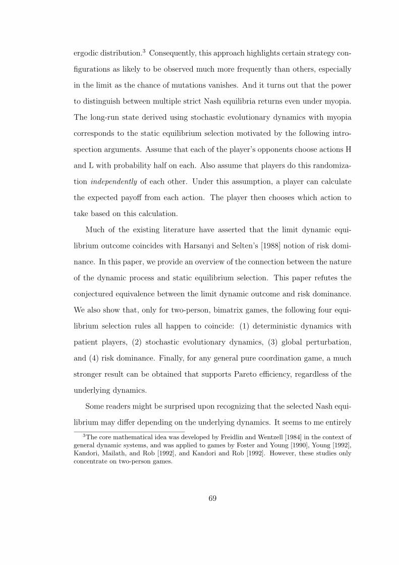
ergodic distribution.3 Consequently, this approach highlights certain strategy con-

figurations as likely to be observed much more frequently than others, especially

in the limit as the chance of mutations vanishes. And it turns out that the power

to distinguish between multiple strict Nash equilibria returns even under myopia.

The long-run state derived using stochastic evolutionary dynamics with myopia

corresponds to the static equilibrium selection motivated by the following intro-

spection arguments. Assume that each of the player’s opponents choose actions H

and L with probability half on each. Also assume that players do this randomiza-

tion independently of each other. Under this assumption, a player can calculate

the expected payoff from each action. The player then chooses which action to

take based on this calculation.

Much of the existing literature have asserted that the limit dynamic equi-

librium outcome coincides with Harsanyi and Selten’s [1988] notion of risk domi-

nance. In this paper, we provide an overview of the connection between the nature

of the dynamic process and static equilibrium selection. This paper refutes the

conjectured equivalence between the limit dynamic outcome and risk dominance.

We also show that, only for two-person, bimatrix games, the following four equi-

librium selection rules all happen to coincide: (1) deterministic dynamics with

patient players, (2) stochastic evolutionary dynamics, (3) global perturbation,

and (4) risk dominance. Finally, for any general pure coordination game, a much

stronger result can be obtained that supports Pareto efficiency, regardless of the

underlying dynamics.

Some readers might be surprised upon recognizing that the selected Nash equi-

librium may differ depending on the underlying dynamics. It seems to me entirely

3The core mathematical idea was developed by Freidlin and Wentzell [1984] in the context ofgeneral dynamic systems, and was applied to games by Foster and Young [1990], Young [1992],Kandori, Mailath, and Rob [1992], and Kandori and Rob [1992]. However, these studies onlyconcentrate on two-person games.

69

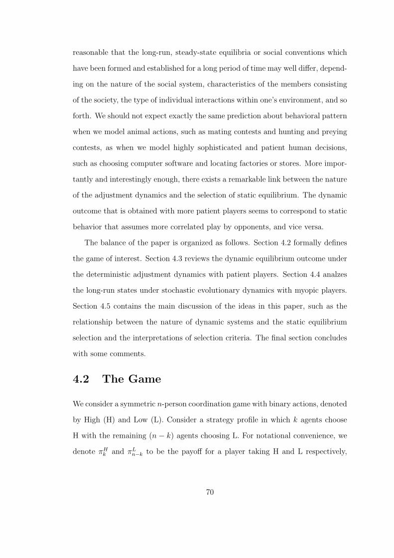
reasonable that the long-run, steady-state equilibria or social conventions which

have been formed and established for a long period of time may well differ, depend-

ing on the nature of the social system, characteristics of the members consisting

of the society, the type of individual interactions within one’s environment, and so

forth. We should not expect exactly the same prediction about behavioral pattern

when we model animal actions, such as mating contests and hunting and preying

contests, as when we model highly sophisticated and patient human decisions,

such as choosing computer software and locating factories or stores. More impor-

tantly and interestingly enough, there exists a remarkable link between the nature

of the adjustment dynamics and the selection of static equilibrium. The dynamic

outcome that is obtained with more patient players seems to correspond to static

behavior that assumes more correlated play by opponents, and vice versa.

The balance of the paper is organized as follows. Section 4.2 formally defines

the game of interest. Section 4.3 reviews the dynamic equilibrium outcome under

the deterministic adjustment dynamics with patient players. Section 4.4 analzes

the long-run states under stochastic evolutionary dynamics with myopic players.

Section 4.5 contains the main discussion of the ideas in this paper, such as the

relationship between the nature of dynamic systems and the static equilibrium

selection and the interpretations of selection criteria. The final section concludes

with some comments.

4.2 The Game

We consider a symmetric n-person coordination game with binary actions, denoted

by High (H) and Low (L). Consider a strategy profile in which k agents choose

H with the remaining (n − k) agents choosing L. For notational convenience, we

denote πHk and πL

n−k to be the payoff for a player taking H and L respectively,

70

where k = 1, . . . , n. The game of interest belongs to:

Ω ≡

Π ∈ <2n | πζk+1 ≥ πζ

k, ∀ ζ, ∀ kwith strict inequality for some k;

πHn > πL

1 , πLn > πH

1 ; πHn ≥ πL

n

. (4.1)

The first set of inequalities in Eq. (4.1) imply that a player taking a particular

action is no worse off when the number of opponents taking the same action

increases. The next two inequalities require that all players playing a common

action be a strict Nash equilibrium. The last inequality means that the equilibrium

when all players play H, denoted by H, is better than the one when all players

play L, denoted by L. Now, the following preliminary result is straightforward:

Lemma 7 If Π ∈ Ω then the only pure strategy equilibria of G(n, Π) are two strict

Nash, viz. H and L.

Proof It suffices to show for all k = 1, . . . , n − 1 both πLn−k > πH

k+1 and πHk >

πLn−k+1 are not satisfied, since otherwise the pure strategy profile of k players

choosing H and (n− k) players choosing L would be Nash. Adding the above two

inequalities yields:

−(πLn−k+1 − πL

n−k) > πHk+1 − πH

k

which contradicts the definition of the Ω set.

All of the Nash refinements, including the strategic stability of Kohlberg

and Mertens, are powerless in selecting between these two strict Nash equilib-

ria. Pareto efficiency is compatible with equilibrium play, so neither an incentive

problem nor conflict exists. However, it is not clear whether players will be able to

reach this outcome in a noncooperative situation where no direct communication

is allowed. In short, strategic uncertainty matters.

71

4.3 Adjustment Dynamics

We begin with the following determinsitic adjustment dynamics, which was orig-

inally introduced by Matsui and Matsuyama [1991] and subsequently studied by

Kim [1992a]. Time is continuous on [0,∞). The game G(n, Π) is played repeat-

edly in a society with a continuum of identical players. At every point in time,

each and every player is matched to form a group with (n− 1) other anonymous

players, who are randomly drawn from the population. All players behave ratio-

nally, choosing a strategy to maximize one’s expected discounted payoff. However,

adjustments are costly, so that players can revise actions only periodically. More

specifically, we assume that the opportunity to switch actions arrives randomly

and independently across players, following a Poisson process with mean arrival

rate λ. This is called an inertia assumption with the speed of adjustment λ.

We allow players to have the chance from time to time to revise their choices

given what their opponents are currently doing, and given the correct expecta-

tion about the future play of the game, namely, perfect foresight. The dynamic

system is deterministic in that there is neither stochastic shocks nor aggregate

uncertainty.

The strategy distribution of the society as of time t can be described by the

state variable yt, the fraction of players that are committed to action H at time

t. The state space thus is [0, 1]. When the opportunity to switch actions arrives,

players choose the action which results in higher expected discounted payoffs, with

respect to the future, expected path of y, as well as their own inability to switch

actions continuously. Let Φ(yt) be the value of playing action H instead of L at

time t. Denote Vt to be discounted expected payoff given perfect foresight path

yt+s, s ≥ 0, i.e.,

Vt ≡ (λ + r)∫ ∞

0Φ(yt+s)e

−(λ+r)sds (4.2)

72

then players will commit to H if Vt > 0 or they will commit to L if Vt < 0, with

indifference optimal if Vt = 0. with r > 0 being the discount factor. We define

r/λ to be the effective discount rate or the degree of friction. To say that the

friction vanishes implies that players are very patient, or that each player can

revise his action whenever he wants. On the other hand, to say that the friction

grows without bound implies that players only care about their immediate gains,

that is players are myopic.

Chapter 3 fully characterizes the dynamic equilibrium outcome in terms of

group size and effective discount rate. We need to introduce the following termi-

nology: A state y is said to be absorbing if a neighborhood U of y exists such that

any equilibrium path from U converges to y. It is said to be globally attractive if

there exists an equilibrium path that reaches or converges to that state from any

initial condition. It can be shown that in the limit as the friction vanishes either

all players playing action H (i.e. y = 1) or all players playing action L (i.e. y = 0)

will be the unique, absorbing and globally attractive state, depending upon the

payoff matrix and group size. More precisely, we restate the following:

Proposition 6 (Kim [1992]) (a) In the limit as players become patient, the

unique, absorbing and globally attractive state selects H if and only if:

1

n

n∑k=1

πHk >

1

n

n∑k=1

πLk (4.3)

with L selected when the inequality is reversed. (b) In the limit as players become

myopic, both H and L can be selected as absorbing states.

Surprisingly, the equilibrium selected coincides with the one selected by Carls-

son and Van Damme’s [1990, 1991] static notion of global perturbation. Trembles

are introduced into the game in such a way that payoffs are almost but not per-

fectly common knowledge, and that there is a chance that each of the actions

73

can be a dominated strategy. More precisely, each player receives a private signal

about the payoffs, but is unable to fully separate the true payoff realization from

one’s private noisy signal. Lack of common knowledge among players makes it

possible for strictly dominated strategies to exert an influence. This fact suggests

that, to solve the resulting incomplete information game, we must use iterative

elimination of strictly dominated strategies. The result of iterative strict domi-

nance prescribes that all players play either H or L, depending on the payoff ma-

trix of the original unperturbed game. Equilibrium selection based upon global

perturbation refers to the one obtained at the exactly original game as common

knowledge about payoffs becomes arbitrarily perfect. To recapitulate, the major

argument of Chapter 3 is that the limiting dynamic outcome is equivalent to the

static equilibrium selection based on global perturbation.

Proposition 6(b) suggests that in the limit as players become myopic exactly

which equilibrium between H and L will be obtained in the long run depends

crucially upon the initial state. In other words, no a priori selection among the

multiple Nash equilibria can be made. How to restore some ability for equilibrium

selection will be discussed in the next section.

4.4 Evolutionary Dynamics

4.4.1 Characterization

For analytical convenience, we modify the repeated societal interactions as follows.

Time is discrete and is denoted by t = 0, 1, . . . , .4 The game G(n, Π) is played

repeatedly in a society with a finite number of identical players N which is an

integer divisible by n. The state variable zt is the number of players adopting

action H at time t, with the state space Z = 0, 1, . . . , N. Let yt = zt/N be

4The analysis extends to a continuous time formulation, as will be mentioned later.

74

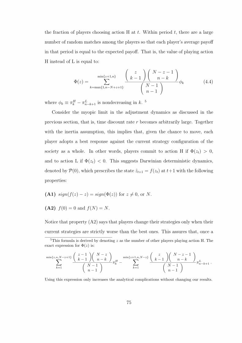
the fraction of players choosing action H at t. Within period t, there are a large

number of random matches among the players so that each player’s average payoff

in that period is equal to the expected payoff. That is, the value of playing action

H instead of L is equal to:

Φ(z) =minz+1,n∑

k=max1,n−N+z+1

(z

k − 1

)(N − z − 1

n− k

)(

N − 1n− 1

) φk (4.4)

where φk ≡ πHk − πL

n−k+1 is nondecreasing in k. 5

Consider the myopic limit in the adjustment dynamics as discussed in the

previous section, that is, time discount rate r becomes arbitrarily large. Together

with the inertia assumption, this implies that, given the chance to move, each

player adopts a best response against the current strategy configuration of the

society as a whole. In other words, players commit to action H if Φ(zt) > 0,

and to action L if Φ(zt) < 0. This suggests Darwinian deterministic dynamics,

denoted by P(0), which prescribes the state zt+1 = f(zt) at t+1 with the following

properties:

(A1) sign(f(z)− z) = sign(Φ(z)) for z 6= 0, or N .

(A2) f(0) = 0 and f(N) = N .

Notice that property (A2) says that players change their strategies only when their

current strategies are strictly worse than the best ones. This assures that, once a

5This formula is derived by denoting z as the number of other players playing action H. Theexact expression for Φ(z) is:

minz,n,N−z+1∑k=1

(z − 1k − 1

)(N − zn− k

)(

N − 1n− 1

) πHk −

minz+1,n,N−z∑k=1

(z

k − 1

)(N − z − 1

n− k

)(

N − 1n− 1

) πLn−k+1 .

Using this expression only increases the analytical complications without changing our results.

75

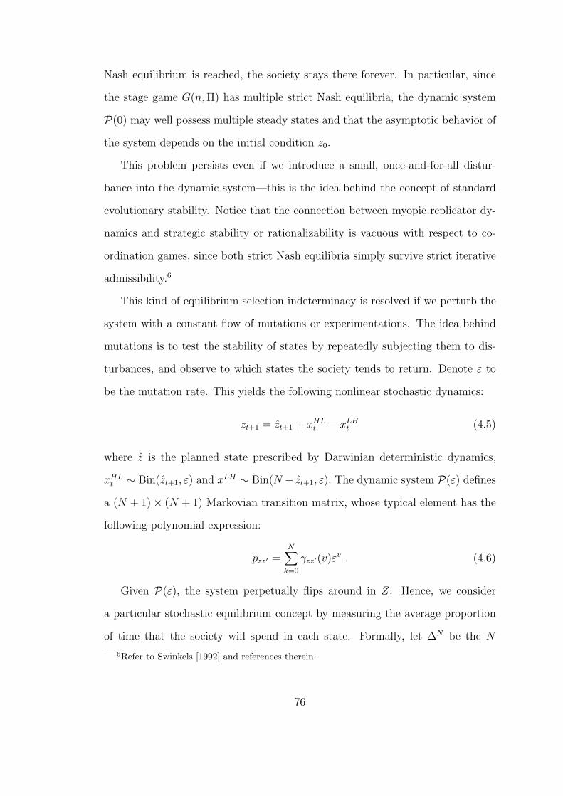
Nash equilibrium is reached, the society stays there forever. In particular, since

the stage game G(n, Π) has multiple strict Nash equilibria, the dynamic system

P(0) may well possess multiple steady states and that the asymptotic behavior of

the system depends on the initial condition z0.

This problem persists even if we introduce a small, once-and-for-all distur-

bance into the dynamic system—this is the idea behind the concept of standard

evolutionary stability. Notice that the connection between myopic replicator dy-

namics and strategic stability or rationalizability is vacuous with respect to co-

ordination games, since both strict Nash equilibria simply survive strict iterative

admissibility.6

This kind of equilibrium selection indeterminacy is resolved if we perturb the

system with a constant flow of mutations or experimentations. The idea behind

mutations is to test the stability of states by repeatedly subjecting them to dis-

turbances, and observe to which states the society tends to return. Denote ε to

be the mutation rate. This yields the following nonlinear stochastic dynamics:

zt+1 = zt+1 + xHLt − xLH

t (4.5)

where z is the planned state prescribed by Darwinian deterministic dynamics,

xHLt ∼ Bin(zt+1, ε) and xLH ∼ Bin(N − zt+1, ε). The dynamic system P(ε) defines

a (N + 1)× (N + 1) Markovian transition matrix, whose typical element has the

following polynomial expression:

pzz′ =N∑

k=0

γzz′(v)εv . (4.6)

Given P(ε), the system perpetually flips around in Z. Hence, we consider

a particular stochastic equilibrium concept by measuring the average proportion

of time that the society will spend in each state. Formally, let ∆N be the N

6Refer to Swinkels [1992] and references therein.

76

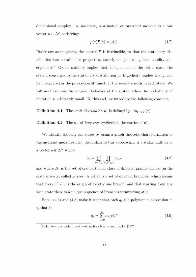
dimensional simplex. A stationary distribution or invariant measure is a row

vector µ ∈ ∆N satisfying:

µ(ε)P(ε) = µ(ε). (4.7)

Under our assumptions, the matrix P is irreducible, so that the stationary dis-

tribution has certain nice properties, namely uniqueness, global stability and

ergodicity.7 Global stability implies that, independent of the initial state, the

system converges to the stationary distribution µ. Ergodicity implies that µ can

be interpreted as the proportion of time that the society spends in each state. We

will next examine the long-run behavior of the system when the probability of

mutation is arbitrarily small. To this end, we introduce the following concepts.

Definition 4.1 The limit distribution µ∗ is defined by limε→0 µ(ε).

Definition 4.2 The set of long run equilibria is the carrier of µ∗.

We identify the long-run states by using a graph-theoretic characterization of

the invariant measures µ(ε). According to this approach, µ is a scalar multiple of

a vector q ∈ ∆N where:

qz =∑

b∈Bz

∏(z′,z′′)∈b

pz′z′′ (4.8)

and where Bz is the set of one particular class of directed graphs defined on the

state space Z, called z-trees. A z-tree is a set of directed branches, which means

that every z′ 6= z is the origin of exactly one branch, and that starting from any

such state there is a unique sequence of branches terminating at z.

Eqns. (4.6) and (4.8) make it clear that each qz is a polynomial expression in

ε, that is:

qz =N∑

v=0

αz(v)εv (4.9)

7Refer to any standard textbook such as Karlin and Taylor [1975].

77

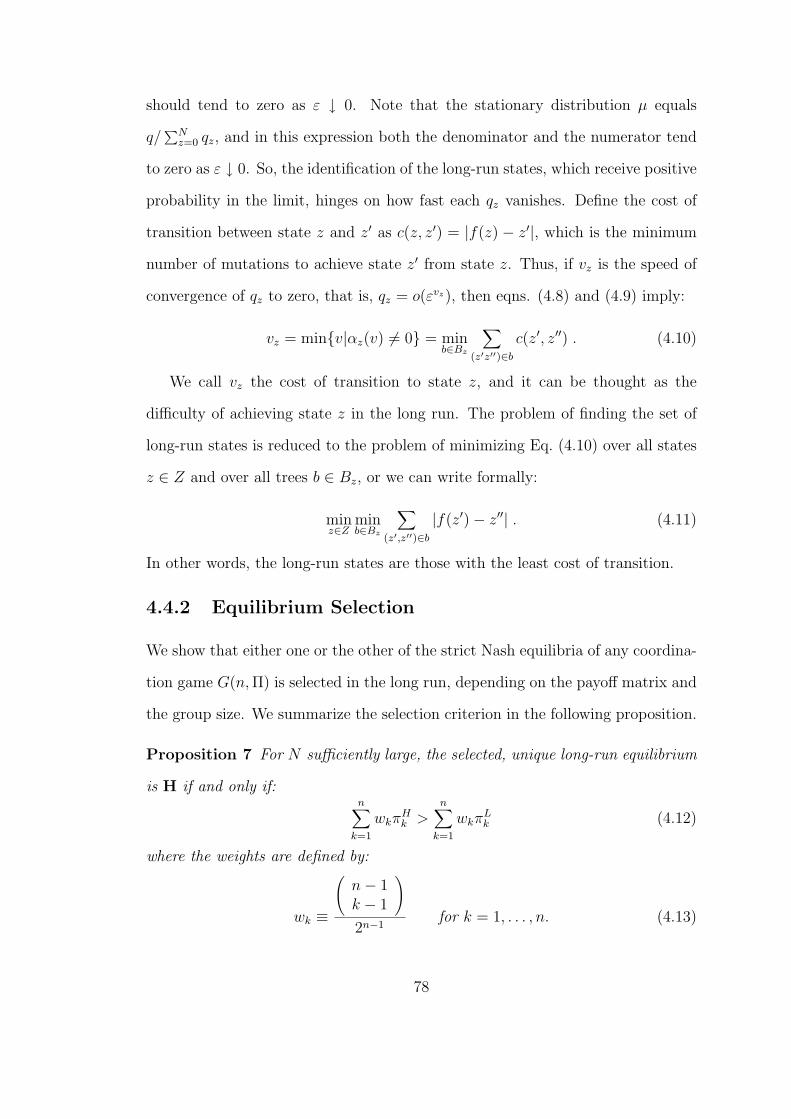
should tend to zero as ε ↓ 0. Note that the stationary distribution µ equals

q/∑N

z=0 qz, and in this expression both the denominator and the numerator tend

to zero as ε ↓ 0. So, the identification of the long-run states, which receive positive

probability in the limit, hinges on how fast each qz vanishes. Define the cost of

transition between state z and z′ as c(z, z′) = |f(z) − z′|, which is the minimum

number of mutations to achieve state z′ from state z. Thus, if vz is the speed of

convergence of qz to zero, that is, qz = o(εvz), then eqns. (4.8) and (4.9) imply:

vz = minv|αz(v) 6= 0 = minb∈Bz

∑(z′z′′)∈b

c(z′, z′′) . (4.10)

We call vz the cost of transition to state z, and it can be thought as the

difficulty of achieving state z in the long run. The problem of finding the set of

long-run states is reduced to the problem of minimizing Eq. (4.10) over all states

z ∈ Z and over all trees b ∈ Bz, or we can write formally:

minz∈Z

minb∈Bz

∑(z′,z′′)∈b

|f(z′)− z′′| . (4.11)

In other words, the long-run states are those with the least cost of transition.

4.4.2 Equilibrium Selection

We show that either one or the other of the strict Nash equilibria of any coordina-

tion game G(n, Π) is selected in the long run, depending on the payoff matrix and

the group size. We summarize the selection criterion in the following proposition.

Proposition 7 For N sufficiently large, the selected, unique long-run equilibrium

is H if and only if:n∑

k=1

wkπHk >

n∑k=1

wkπLk (4.12)

where the weights are defined by:

wk ≡

(n− 1k − 1

)2n−1

for k = 1, . . . , n. (4.13)

78

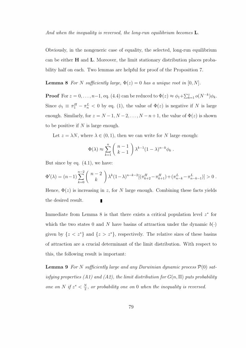
And when the inequality is reversed, the long-run equilibrium becomes L.

Obviously, in the nongeneric case of equality, the selected, long-run equilibrium

can be either H and L. Moreover, the limit stationary distribution places proba-

bility half on each. Two lemmas are helpful for proof of the Proposition 7.

Lemma 8 For N sufficiently large, Φ(z) = 0 has a unique root in [0, N ].

Proof For z = 0, . . . , n−1, eq. (4.4) can be reduced to Φ(z) ≈ φ1+∑z

k=1 o(N−k)φk.

Since φ1 ≡ πH1 − πL

n < 0 by eq. (1), the value of Φ(z) is negative if N is large

enough. Similarly, for z = N − 1, N − 2, . . . , N −n+1, the value of Φ(z) is shown

to be positive if N is large enough.

Let z = λN , where λ ∈ (0, 1), then we can write for N large enough:

Φ(λ) ≈n∑

k=1

(n− 1k − 1

)λk−1(1− λ)n−kφk .

But since by eq. (4.1), we have:

Φ′(λ) = (n−1)n−2∑k=0

(n− 2

k

)λk(1−λ)n−k−2[(πH

k+2−πHk+1)+(πL

n−k−πLn−k−1)] > 0 .

Hence, Φ(z) is increasing in z, for N large enough. Combining these facts yields

the desired result.

Immediate from Lemma 8 is that there exists a critical population level z∗ for

which the two states 0 and N have basins of attraction under the dynamic b(·)

given by z < z∗ and z > z∗, respectively. The relative sizes of these basins

of attraction are a crucial determinant of the limit distribution. With respect to

this, the following result is important:

Lemma 9 For N sufficiently large and any Darwinian dynamic process P(0) sat-

isfying properties (A1) and (A2), the limit distribution for G(n, Π) puts probability

one on N if z∗ < N2, or probability one on 0 when the inequality is reversed.

79

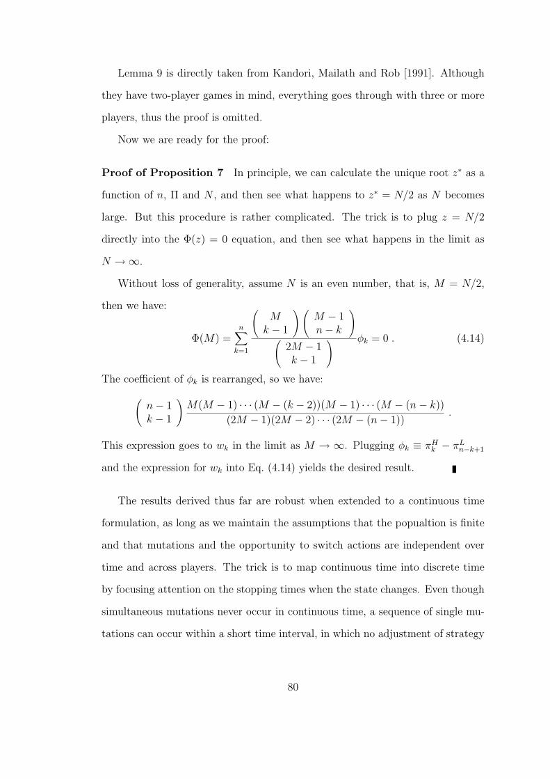
Lemma 9 is directly taken from Kandori, Mailath and Rob [1991]. Although

they have two-player games in mind, everything goes through with three or more

players, thus the proof is omitted.

Now we are ready for the proof:

Proof of Proposition 7 In principle, we can calculate the unique root z∗ as a

function of n, Π and N , and then see what happens to z∗ = N/2 as N becomes

large. But this procedure is rather complicated. The trick is to plug z = N/2

directly into the Φ(z) = 0 equation, and then see what happens in the limit as

N →∞.

Without loss of generality, assume N is an even number, that is, M = N/2,

then we have:

Φ(M) =n∑

k=1

(M

k − 1

)(M − 1n− k

)(

2M − 1k − 1

) φk = 0 . (4.14)

The coefficient of φk is rearranged, so we have:(n− 1k − 1

)M(M − 1) · · · (M − (k − 2))(M − 1) · · · (M − (n− k))

(2M − 1)(2M − 2) · · · (2M − (n− 1)).

This expression goes to wk in the limit as M → ∞. Plugging φk ≡ πHk − πL

n−k+1

and the expression for wk into Eq. (4.14) yields the desired result.

The results derived thus far are robust when extended to a continuous time

formulation, as long as we maintain the assumptions that the popualtion is finite

and that mutations and the opportunity to switch actions are independent over

time and across players. The trick is to map continuous time into discrete time

by focusing attention on the stopping times when the state changes. Even though

simultaneous mutations never occur in continuous time, a sequence of single mu-

tations can occur within a short time interval, in which no adjustment of strategy

80

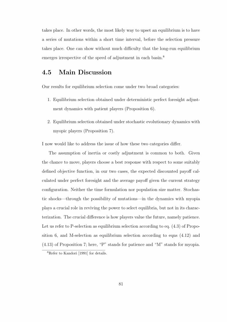
takes place. In other words, the most likely way to upset an equilibrium is to have

a series of mutations within a short time interval, before the selection pressure

takes place. One can show without much difficulty that the long-run equilibrium

emerges irrespective of the speed of adjustment in each basin.8

4.5 Main Discussion

Our results for equilibrium selection come under two broad categories:

1. Equilibrium selection obtained under deterministic perfect foresight adjust-

ment dynamics with patient players (Proposition 6).

2. Equilibrium selection obtained under stochastic evolutionary dynamics with

myopic players (Proposition 7).

I now would like to address the issue of how these two categories differ.

The assumption of inertia or costly adjustment is common to both. Given

the chance to move, players choose a best response with respect to some suitably

defined objective function, in our two cases, the expected discounted payoff cal-

culated under perfect foresight and the average payoff given the current strategy

configuration. Neither the time formulation nor population size matter. Stochas-

tic shocks—through the possibility of mutations—in the dynamics with myopia

plays a crucial role in reviving the power to select equilibria, but not in its charac-

terization. The crucial difference is how players value the future, namely patience.

Let us refer to P-selection as equilibrium selection according to eq. (4.3) of Propo-

sition 6, and M-selection as equilibrium selection according to eqns (4.12) and

(4.13) of Proposition 7; here, “P” stands for patience and “M” stands for myopia.

8Refer to Kandori [1991] for details.

81

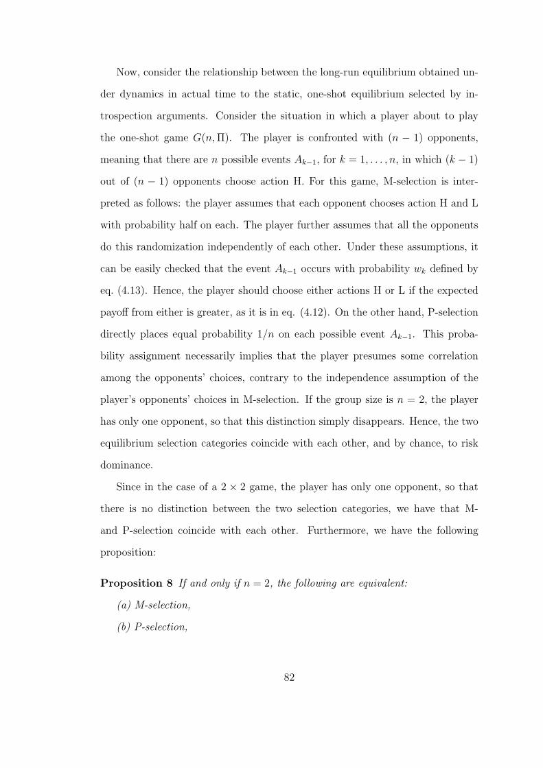
Now, consider the relationship between the long-run equilibrium obtained un-

der dynamics in actual time to the static, one-shot equilibrium selected by in-

trospection arguments. Consider the situation in which a player about to play

the one-shot game G(n, Π). The player is confronted with (n − 1) opponents,

meaning that there are n possible events Ak−1, for k = 1, . . . , n, in which (k − 1)

out of (n − 1) opponents choose action H. For this game, M-selection is inter-

preted as follows: the player assumes that each opponent chooses action H and L

with probability half on each. The player further assumes that all the opponents

do this randomization independently of each other. Under these assumptions, it

can be easily checked that the event Ak−1 occurs with probability wk defined by

eq. (4.13). Hence, the player should choose either actions H or L if the expected

payoff from either is greater, as it is in eq. (4.12). On the other hand, P-selection

directly places equal probability 1/n on each possible event Ak−1. This proba-

bility assignment necessarily implies that the player presumes some correlation

among the opponents’ choices, contrary to the independence assumption of the

player’s opponents’ choices in M-selection. If the group size is n = 2, the player

has only one opponent, so that this distinction simply disappears. Hence, the two

equilibrium selection categories coincide with each other, and by chance, to risk

dominance.

Since in the case of a 2 × 2 game, the player has only one opponent, so that

there is no distinction between the two selection categories, we have that M-

and P-selection coincide with each other. Furthermore, we have the following

proposition:

Proposition 8 If and only if n = 2, the following are equivalent:

(a) M-selection,

(b) P-selection,

82

(c) global perturbation,

(c) risk dominance.

Proof The preceding arguments in the text above imply that (a) and (b) coincide

when n = 2. Equivalence between (b) and (c) is true in general Chapter 4.3 of

this paper. Carlsson and Van Damme [1990] verify the equivalence between (c)

and (d) for two-person, bimatrix games.

The limit behavior of Blume’s [1991] dynamic process with respect to parametric

changes making strategy revisions a best response is shown to give rise to the

same outcome as risk dominance in 2× 2 coordination games. Kandori, Mailath,

and Rob [1992]—upon which our Section 4 depends heavily—and Fudenberg and

Harris [1992] show that, in 2×2 games, as the mutation rate and noise go to zero,

the ergodic distribution becomes concentrated on the risk dominant equilibrium.9

Lastly, Matsui and Matsuyama [1991]—from which our model borrows heavily—

shows an equivalence between risk dominance and dynamic stability in 2 × 2

games of common interest. From the viewpoint of Proposition 8 above, the first

three papers (i.e. Blume, KMR and FH) claim nothing but the equivalence be-

tween M-selection and risk dominance, with the last paper (ie, MM) claiming the

equivalence between P-selection and risk dominance.

We now study a generalized pure-coordination or simply voting game, where

the payoff to the player playing action s = 1, 2, . . . ,m is described as follows:

πs(](1), ..., ](m)) =

as if ](s) ≥ κ0 otherwise

where ](s) denotes the total number of players choosing action s, and κ may be

2, .., n. Moerover, all coordinated equilibria are ordered, that is, 0 ≤ as ≤ as′ , ∀s <

9Fudenberg and Harris needs to be read with some care, since in this paper, the population islarge and the random perturbation is introduced by a Brownian motion, so that the stochasticshocks are necessarily correlated across players. This is in sharp contrast to our assumptionconcerning the independence of the random shocks across players and over time.

83

s′. This class of games, denoted G(n, m; Πκ) to emphasize the importance of κ.

possesses m pure strategy Pareto rankable Nash equilibria, everyone’s choosing

action s = 1, 2, ...,m. It requires that both the voting rule (represented by κ) and

the security (normalized to zero) be identical over all choices. Then we have:10

Proposition 9 In any G(n, m; Πκ), the Pareto efficient Nash equilibrium is sup-

ported, regardless of the underlying dynamics.

Proof is lengthy, but the idea is intuitive. The previous sections suggest that

Pareto efficiency is guaranteed when the number of actions is two, i.e. m = 2.

With three or more actions, we apply the selection criterion in a pairwise way.

The only case that we have to worry about is lack of transitivities, but this cannot

occur in the present class of games.

proof

(1) Deterministic Adjustment Dynamic with Patient Players:

All the proofs of Section 3 apply straightforwardly, so we omit them. After all,

we are able to show that: if ρ ∈ (0, ρ], then the Pareto efficient outcome is

uniquely absorbing and globally attractive and thus is robust with respect to

global perturbation.

(2) Stochastic Evolutionary Dynamics:

Given a chance to move and the state z = (z1, ..., zm), the expected average

payoff for the player who has been choosing action s is calculated asfκ(z

s − 1)as if he chooses s againfκ(z

s′)as′ if he chooses s′ 6= s(4.15)

10We can easily construct counterexamples demonstrating the fact that both identical ruleand equal security are necessary and sufficient to guarantee the Pareto efficiency.

84

where

fκ(z) =minz+1,n∑

k=max1,n−N+z+1

(z

k − 1

)(N − z − 1

n− k

)(

N − 1n− 1

) , z ∈ Z ≡ 0, 1, ..., N

(4.16)

The next lemma is just a technical result but plays an important role in what

follows.

Lemma 10 For any κ, the function fκ(z) is strictly increasing in z ∈ Z.

Proof Via mathematical induction. Without loss of generality, assume z ∈

n− 1, n, ..., N − n. For κ = n, a direct calculation shows that

fn(z)− fn(z − 1) =

(z − 1n− 2

)(N − z − 1

0

)> 0.

Now suppose it is true for κ + 1 that

fκ+1(z)− fκ+1(z − 1) =

(z − 1κ− 1

)(N − z − 1n− κ− 1

),

then

fκ(z)− fκ(z − 1)

= [fκ+1(z)− fκ+1(z − 1)] + [

(z

κ− 1

)(N − z − 1

n− κ

)−(

z − 1κ− 1

)(N − zn− κ

)]

=

(z

κ− 1

)(N − z − 1

n− κ

)− [

(z − 1κ− 1

)(N − zn− κ

)−(

z − 1κ− 1

)(N − z − 1n− κ− 1

)]

=

(z − 1κ− 2

)(N − z − 1

n− κ

)> 0.

Lemma 11 Any mixed strategy is unstable.

Proof Assume not, i.e. there exist s, s′ ∈ C(z) with s < s′, and both s and s′

are best reponses to z. Then we get

f(zs′ − 1)as′ ≥ f(zs)as > f(zs − 1)as ≥ f(zs′)as′ > f(zs′ − 1)as′ .

85

The strict inequalities follow from Lemma 7 and the weak inequalities follow from

the presumed optimality of s and s′ relative to z. The contracdiction establishes

the desired result.

Lemma 12 The collection of limit sets is esms=1.

This last lemma states that the Darwinian dynamic for the game G(n, m; Πκ)

converges to a pure strategy Nash configuration with probability one. The same

logic as in Proposition 7(2) of KR applies, so proof is omitted. Now we are ready

to verify the Pareto efficiency under stochastic evolutionary dynamics:

Recalling Eq. (16), the first task is to compute costs of transition Cs′s between limit

sets, es and es′ . Assume the society is initially clustered at es′ , then the minimum

number of mutations, x, needed to switch it over into the basin of attraction of es

is determined by f(x)as ≥ f(N − 1 − x)as′ . This represents an immediate jump

to escape the best response region of s′, and the triangular inequality argument

of KR’s Proposition 5 guarantees that no gradual escape is less costly than this

immediate jump. Note that we mutate individuals taking s′ into s, because any

other mutation will only raise the transition cost more. Thus, the cost of transition

Cs′s is the minimum integer x satisfying

f(x) ≥ f(N − 1− x)as′

as

(4.17)

It has a unique root, since Lemma 7 implies that the left hand side of Eq. (31) is

strictly increasing and so its right hand side is strictly decreasing in x.

Since a pure coordination game G(n, m; Πκ) specifies 0 ≤ a1 ≤ a2 ≤ · · · ≤ am,

we can easily check that

Cs′m < Cs′s, ∀s < m,∀s′ 6= s, and Cm,m−1 < Cs′,m−1, ∀s′ < m− 1.

86

Therefore, the first step of the optimum branching algorithm as in Appendix B of

KR is to choose a minimum cost outgoing branch from each state, which results

in the system of branches (s → m), s = 1, 2, ...,m − 1, and (m → m − 1). The

longest branch among these is of length Cm,m−1. Therefore we drop it, and are

left with an m-tree. This completes the algorithm.

Corollary 4 In any pure coordination game, the dynamic equilibrium outcome

selects the Pareto-efficient outcome H, irrespective of the details of the underlying

adjustment dynamics.

4.6 Final Remarks

We have generalized results on equilibrium selection in the direction of group

size. However, the assumption of binary strategies is obviously restrictive. A full

characterization of the long-run states for broader classes of games beyond those

studied in this paper seems difficult, because of the numerous case distinctions and

complicated calculations. This is the reason why Kandori and Rob [1992] ends up

only solving the two-player, three-action supermodular game. Yet, it does seem

valuable to characterize the general properties of the long-run states for broader

classes of multiperson games, such as multiperson supermodular games. We will

have to await further research in this direction for answers.

87

Chapter 5

Reference

88

1. L. Anderlini and H. Sabourian, Cooperation and Effective Computabil-

ity, mimeo, University of Cambridge, 1991.

2. R.J. Aumann and S. Sorin, Cooperation and Bounded Recall, Games

and Economic Behavior 1 (1989), 5-39.

3. K. Binmore and L. Samuelson, Evolutionary Games in Repeated Games

Played by Finite Automata, Journal of Economic Theory 57 (1992), 278-305.

4. L. Blume, The Statistical Mechanics of Strategic Interactions, mimeo, Cor-

nell University, 1991.

5. L. Blume and D. Easley, Evolution and Market Behavior, Journal of

Economic Theory (1992), 9-40.

6. R. T. Boylan, Continuous Approximation of Dynamical Systems with

Randomly Matched Individuals, mimeo, Washington University, 1992.

7. Bulow, J., and K. Rogoff, Sovereign Debt: Is to Forgive to Forget ?,

American Economic Review 79 (1989a), 43-50.

8. ————————–(1989b), A Constant Recontracting Model of Sovereign

Debt, Journal of Political Economy 97, 155-78.

9. Camerer, C., and K. Weigelt, Experimental Tests of a Sequential

Equilibrium Reputation Model, Econometrica 56 (1988), 1-36.

10. D. Canning, Average Behavior in Learning Models, Journal of Economic

Theory, 57 (1992), 442-72.

11. H. Carlsson and E. van Damme, Global Games and Equilibrium Se-

lection, CenTER # 9052, Tilburg University, 1990.

89

12. ——————————- , Equilibrium Selection in Stag Hunt Games, Cen-

TER # 9170, Tilburg University, 1991.

13. R. W. Cooper, D. V. DeJong, R. Forsythe, and T. W. Ross, Selec-

tion Criteria in Coordination Games: Some Experimental Results, American

Economic Review 80 (1990), 218-33.

14. ——————————- , Communication in Coordination Games, Quar-

terly Journal of Economics 107 (1992), 739-71.

15. V. Crawford, An Evolutionary Interpretation of Van Huyck, Battalio,

and Beil’s experimental results on coordination games, Games and Economic

Behavior 3 (1991), 25-59.

16. D. Diamond, Reputation Acquisition in Debt Markets, Journal of Political

Economy (1989), 828-62.

17. G. Ellison, Learning, Local Interaction, and Coordination, mimeo, MIT,

1991.

18. G. Ellison and D. Fudenberg, Rules of Thumb for Social Learning,

mimeo, MIT, 1992.

19. G.W. Evans and R. Guesnerie, Rationalizability, Strong Rationality,

and Expectational Stability, mimeo, London School of Economics, 1992.

20. D. Foster and P. Young, Stochastic Evolutionary Game Dynamics,”

Theoretical Population Biology 38 (1990), 219-32.

21. Freidlin, M. I., and A. D. Wentzell, Random Perturbations of Dy-

namical Systems, Springer-Verlag, New York, 1984.

90

22. D. Fudenberg, Explaining Cooperation and Commitment in Repeated

Games, in J.-J. Laffont (eds.), Advances in Economic Theory Vol.I: Sixth

World Congress of the Econometric Society, Cambridge University Press,

1992.

23. D. Fudenberg and C. Harris, Evolutionary Dynamics with Aggregate

Shocks, Journal of Economic Theory, 57 (1992), 420-41.

24. D. Fudenberg and D. Kreps, Reputation in the Simultaneous Play of

Multiple Opponents, Review of Economic Studies (1987), 541-68.

25. —————————————-, Lecture on Learning and Equilibrium in Strate-

gic Form Games, CORE Lecture Series, Belgium, 1992a.

26. —————————————-, Learning Mixed Equilibria, mimeo, Stan-

ford Graduate School of Business and MIT, 1992b.

27. D. Fudenberg, D. Kreps and D. K. Levine, On the Robustness of

Equilibrium Refinements, J. Economic Theory 48 (1988), 261-79.

28. D. Fudenberg, D. Kreps, and E. Maskin, Repeated Games with Long

and Short run Players, Review Economic Studies (1990), 555-73.

29. D. Fudenberg and D. K. Levine, Reputation and Equilibrium Selection

in Games with a Patient Player, Econometrica 57 (1989a), 759-78.

30. ——————————————-, Efficiency and Observability with Long-

run and Short-run Players, mimeo, MIT and UCLA, 1989b.

31. ——————————————-, Reputation when Strategies Are Unob-

served, Review Economic Studies (1992a).

91

32. ——————————————-, Steady State Learning and Nash Equilib-

rium, mimeo, MIT and UCLA, 1992b.

33. ——————————————-, Self-Confirming Equilibria, mimeo, MIT

and UCLA, 1992c.

34. I. Gilboa and A. Matsui, Social Stability and Equilibrium, Econometrica

59 (1991), 859-67.

35. N.S. Glance and B.A. Huberman, Dynamics of Social Dilemmas, mimeo,

Xerox Palo Alto Research Center, California, 1992.

36. E. Green, Individual Level Randomness in a Nonatomic Population, mimeo,

University of Pittsburgh, 1989.

37. S. Grossman, The Informational Role of Warranties and Private Disclosure

about Product Quality, Journal of Law and Economics (1981), 461-83.

38. G. W. Harrison and J. Hirshleifer, An Experimental Evaluation of

Weakest Link/Best Shot Models of Public Goods, J. Political Economy 97

(1989), 201-25.

39. J. C. Harsanyi, Games with Randomly Disturbed Payoffs: A New Ratio-

nale for Mixed Strategy Equilibrium Points, International Journal of Game

Theory 2 (1973), 1-23.

40. J. C. Harsanyi and R. Selten, A General Theory of Equilibrium Selec-

tion in Games, MIT Press, Massachussetts, 1988.

41. O. Hart and J. Tirole, Contract Renegotiation and Coasian Dynamics,

Review of Economic Studies (1988), 509-40.

92

42. Hofbauer, J., and K. Sigmund, The Theory of Evolution and

Dynamical Systems, Cambridge University Press, London, 1988.

43. J. Jordan, Bayesian Learning in Normal Form Games, Games and Eco-

nomic Behavior 3 (1991), 60-81.

44. E. Kalai and E. Lehrer, Rational Learning Leads to Nash Equilibrium,

mimeo, Northwertern University, 1991.

45. M. Kandori, Independent Mutations and Long Run Equilibria in Games:

A Continuous Time Formulation,” mimeo, Princeton University, 1991.

46. ——————–, Social Norms and Community Enforcement, Review of Eco-

nomic Studies 59 (1992), 63-80.

47. M. Kandori, G. Mailath, and R. Rob, Learning, Mutation and Long

Equilibria in Games, forthcoming Econometrica, 1992.

48. M. Kandori and R. Rob, Evolution of Equilibria in the Long Run: A

General Theory and Applications, mimeo, Princeton University, 1992.

49. S. Karlin and H. M. Taylor, A First Course in Stochastic Processes,

Academic Press, San Diego, 1975.

50. Y. Kim, Characterization and Properties of Reputation Effects in Extensive

Form Games, mimeo, UCLA, 1990.

51. —————, Adjustment Dynamics with Patient Players in Coordination

Games, working paper #667, UCLA, 1992a.

52. —————, Adjustment, Evolution, and Equilibrium Selection in Games,

mimeo, UCLA, 1992b.

93

53. B. Klein and K. Leffler, The Role of Market Forces in Assuring Con-

tractual Performance, Journal of Political Economy 89 (1981), 615-41.

54. E. Kohlberg and J.-F. Mertens, On the Strategic Stability of Equilib-

ria, Econometrica 54 (1986), 1003-38.

55. D. Kreps, Game Theory and Economic Modelling, Clarendon Lectures in

Economics, Oxford University Press, 1990.

56. D. Kreps and R. Wilson, Sequential Equilibrium, Econometrica 50

(1982a), 863-94.

57. ———————————–, Reputation and Imperfect Information, Journal

of Economic Theory 27 (1982b), 253-79.

58. V. Krishna, Games with Strategic Complementaritiies, mimeo, Harvard

Business School, 1992.

59. P. Krugman, Geography and Trade, MIT Press, Massachussetts, 1991.

60. G.J. Mailath, Introduction: Symposium on Evolutionary Game Theory,

Journal of Economic Theory 57 (1992), 259-77.

61. A. Matsui, Cheap Talk and Cooperation in Society, Journal of Economic

Theory 54 (1991), 245-58.

62. —————, Best Response Dynamics and Socially Stable Strategies, J. Eco-

nomic Theory 57 (1992), 343-62.

63. A. Matsui and K. Matsuyama, An Approach to Equilibrium Selection,

Hoover Institution Working Paper E-91-14, Stanford University, 1991.

94

64. A. Matsui and R. Rob, Evolution, Rationality, and Equilibrium Selection

in Societal Games, mimeo, University of Pennsylvania, 1991.

65. P. Milgrom and J. Roberts, Predation, Reputation, and Entry Deter-

rence, Journal of Economic Theory 27 (1982), 280-312.

66. —————————————, Rationalizability, Learning, and Equilibrium

in Games with Strategic Complementarities, Econometrica 58 (1990), 1255-

77.

67. —————————————, Adaptive and Sophisticated Learning in Re-

peated Normal Form Games, Games and Economic Behavior 3 (1991), 82-

100.

68. M.A. Nowak and R.M. May, Evolutionary Games and Spatial Chaos,

Nature 359 (October 1992), 826-9.

69. A. Rubinstein, The Electronic Mail Games: Strategic Behavior under

“Almost Common Knowledge,” American Economic Review 79 (1989), 385-

91.

70. L. Samuelson, How to Tremble if You Must, mimeo, University of Wis-

consin, 1991.

71. T. Schelling, The Strategy of Conflict, Harvard University Press, Mas-

sachussetts, 1960.

72. K.M. Schmidt, Commitment through Incomplete Information in a Simple

Repeated Bargaining Model, mimeo, 1990.

73. ———————–, Reputation in Games with Conflicting Interest, forthcom-

ing in Journal of Economic Theory, 1992.

95

74. R. Selten, The Chain Store Paradox, Theory and Decision 9 (1977), 127-

59.

75. L.S. Shapley, Some Topics in Two-person Games, Annals of Mathematics

Studies 5 (1964), 1-28.

76. J. Swinkels, Evolutionary Stability With Equilibrium Entrants, J. Eco-

nomic Theory 57 (1992a), 306-32.

77. —————–, Adjustment Dynamics and Rational Play in Games, mimeo,

Stanford University, 1992b.

78. H.P. Young, The Evolution of Conventions, forthcoming in Econometrica,

(1992).

79. H.P. Young and D. Foster, Cooperation in the Short and in the Long

run, Games and Economic Behavior 3 (1991), 145-56.

80. J. B. van Huyck, R. C. Battalio, and R. O. Beil, Tacit Coordi-

nation Games, Strategic Uncertainty, and Coordination Failure, American

Economic Review 80 (1990), 234-48.

81. —————————————-, Strategic Uncertainty, Equilibrium Selection,

and Coordination Failure in Average Opinion Games, Quarterly J. Eco-

nomics 106 (1991), 885–910.

96