Learning error-correcting representations

for multi-class problems

Miguel Ángel Bautista Martín

Aquesta tesi doctoral està subjecta a la llicència Reconeixement 3.0. Espanya de Creative Commons. Esta tesis doctoral está sujeta a la licencia Reconocimiento 3.0. España de Creative Commons. This doctoral thesis is licensed under the Creative Commons Attribution 3.0. Spain License.

Learning Error-Correcting Representationsfor Multi-Class Problems

A dissertation submitted by Miguel ÁngelBautista Martín at Universitat de Barcelona tofulfil the degree of Doctor en Matemàtiques.

Barcelona, November 25, 2015

Director Dr. Sergio EscaleraDept. Matemàtica Aplicada i AnálisiUniversitat de Barcelona

Co-director Dr. Oriol PujolDept. Matemàtica Aplicada i AnálisiUniversitat de Barcelona

This document was typeset by the author using LATEX2ε.

The research described in this book was carried out at Dept. Matemàtica Aplicada iAnálisi, Universitat de Barcelona and the Computer Vision Center, Universitat Autònomade Barcelona.

Copyright c© 2015 by Miguel Ángel Bautista Martín. All rights reserved. No part of thispublication may be reproduced or transmitted in any form or by any means, electronic ormechanical, including photocopy, recording, or any information storage and retrieval system,without permission in writing from the author.

ISBN: XXXXX

Printed by Ediciones Gráficas Rey, S.L.

A mis padres y hermana de los que aprendo cada dıa.

ii

Acknowledgements

As most things in life, this dissertation is the result of certain people allocated in certain timeand place, I would like to thank all of them here. First and foremost I am deeply thankfulto my supervisors Dr. Sergio Escalera and Dr. Oriol Pujol for their motivation, hard workand efforts during all these years, this would have not been possible without them. I wouldalso like to thank Dr. Xavier Baró for his guidance and comments.

Staying at the Human Sensing group Carnegie Mellon University I had the chance to meetDr. Fernando de la Torre to whom I am very thankful for sharing his experience, knowledgeand overall working process with me. I am also very thankful to the bright students thatI met there and with whom I enjoyed a lot of very nice discussions. Amongst them all, Iwould like to thank Ricardo, Paco and Ishan for sharing their comments and experiences withme. I also would like to thank to all the people at the Applied Mathematics and Analysisdepartment at University of Barcelona: Francesco, Piero, Adriana, Víctor, Jordi, Petia, Eloiy Laura. All of you shared your moments, experiences and discussions with me, making mea better scientist.

Engaging in the birth of the Human Pose and Behavior Analysis (HuPBA) group at theUniversity of Barcelona, was one of the best scientific experiences I have ever had. I amdeeply thankful to all my colleagues at the HuPBA group. In particular, to Toni, Xavi,Victor and Albert. Not only did I learn from their hard-work, dedication and knowledge butI also shared with them great memories that I will hold dear forever.

Levemente, quisiera tomarme unas líneas en español para agradecer a todos mis amigos enIbiza y Barcelona que durante estos años han estado a mi lado haciendo que el camino fueramás fácil. En primer lugar querría agradecer a Pau los momentos que hemos compartidojuntos durante todos estos años. También me gustaría agradecer a Adri, Adrián y Javipor los años compartidos en Barcelona. A todas las nuevas amistades hechas en Barcelona:Jordi, Óscar, Christian, Daniel, David, Vicente, Borja, Víctor, Oriol, y un largo etcétera queocuparía varias páginas. Finalmente, quiero agradecer a mis padres Ana y Miguel por laeducación que me han dado así como por los valores de humildad, esfuerzo y honestidad quesiempre me han inculcado.

A mi hermana Ana quiero dedicarle no solo esta línea sino la tesis en su totalidad, es unejemplo para mí.

iii

iv

Two monks were watching a flag flapping inthe wind. One said to the other, "The flag ismoving." The other replied, "The wind ismoving." the sixth and last patriarch of ChánBuddhism who was happening to pass by,overheard this. He said, "Not the flag, notthe wind; mind is moving."

Case 29 - The Gateless Gate

Abstract

Real life is full of multi-class decision tasks. In the Pattern Recognition field, several method-ologies have been proposed to deal with binary problems obtaining satisfying results in termsof performance. However, the extension of very powerful binary classifiers to the multi-classcase is a complex task. The Error-Correcting Output Codes framework has demonstrated tobe a very powerful tool to combine binary classifiers to tackle multi-class problems. However,most of the combinations of binary classifiers in the ECOC framework overlook the underlay-ing structure of the multi-class problem. In addition, is still unclear how the Error-Correctionof an ECOC design is distributed among the different classes.

In this dissertation, we are interested in tackling critic problems of the ECOC framework,such as the definition of the number of classifiers to tackle a multi-class problem, how toadapt the ECOC coding to multi-class data and how to distribute error-correction amongdifferent pairs of categories.

In order to deal with this issues, this dissertation describes several proposals. 1) Wedefine a new representation for ECOC coding matrices that expresses the pair-wise codewordseparability and allows for a deeper understanding of how error-correction is distributedamong classes. 2) We study the effect of using a logarithmic number of binary classifiersto treat the multi-class problem in order to obtain very efficient models. 3) In order tosearch for very compact ECOC coding matrices that take into account the distribution ofmulti-class data we use Genetic Algorithms that take into account the constraints of theECOC framework. 4) We propose a discrete factorization algorithm that finds an ECOCconfiguration that allocates the error-correcting capabilities to those classes that are moreprone to errors.

The proposed methodologies are evaluated on different real and synthetic data sets: UCIMachine Learning Repository, handwriting symbols, traffic signs from a Mobile MappingSystem, and Human Pose Recovery. The results of this thesis show that significant perfor-mance improvements are obtained on traditional coding ECOC designs when the proposedECOC coding designs are taken into account.

v

vi

Resumen

En la vida cotidiana las tareas de decisión multi-clase surgen constantemente. En el campode Reconocimiento de Patrones muchos métodos de clasificación binaria han sido propuestosobteniendo resultados altamente satisfactorios en términos de rendimiento. Sin embargo,la extensión de estos sofisticados clasificadores binarios al contexto multi-clase es una tareacompleja. En este ámbito, las estrategias de Códigos Correctores de Errores (CCEs) handemostrado ser una herramienta muy potente para tratar la combinación de clasificadoresbinarios. No obstante, la mayoría de arquitecturas de combinación de clasificadores binariosnegligen la estructura del problema multi-clase. Sin embargo, el análisis de la distribuciónde corrección de errores entre clases es aún un problema abierto.

En esta tesis doctoral, nos centramos en tratar problemas críticos de los códigos correc-tores de errores; la definición del numero de clasificadores necesarios para tratar un problemamulti-clase arbitrario; la adaptación de los problemas binarios al problema multi-clase y cómodistribuir la corrección de errores entre clases. Para dar respuesta a estas cuestiones, en estatesis doctoral describimos varias propuestas. 1) Definimos una nueva representación paraCCEs que expresa la separabilidad entre pares de códigos y nos permite una mejor com-prensión de cómo se distribuye la corrección de errores entre distintas clases. 2) Estudiamosel efecto de usar un numero logarítmico de clasificadores binarios para tratar el problemamulti-clase con el objetivo de obtener modelos muy eficientes. 3) Con el objetivo de en-contrar modelos muy eficientes que tienen en cuenta la estructura del problema multi-claseutilizamos algoritmos genéticos que tienen en cuenta las restricciones de los ECCs. 4) Pro-ponemos un algoritmo de factorización de matrices discreta que encuentra ECCs con unaconfiguración que distribuye corrección de error a aquellas categorías que son más propensasa tener errores.

Las metodologías propuestas son evaluadas en distintos problemas reales y sintéticoscomo por ejemplo: Repositorio UCI de Aprendizaje Automático, reconocimiento de sím-bolos escritos, clasificacion de señales de trafico y reconocimiento de la pose humana. Losresultados obtenidos en esta tesis muestran mejoras significativas en rendimiento comparadoscon los diseños tradiciones de ECCs cuando las distintas propuestas se tienen en cuenta.

vii

viii

Contents

1 Introduction 11.1 Motivation . . . . . . . . . . . . . . . . . . . . . . . . . . . . . . . . . . . . . 21.2 Statistical Pattern Recognition . . . . . . . . . . . . . . . . . . . . . . . . . . 3

1.2.1 Visual Pattern Recognition . . . . . . . . . . . . . . . . . . . . . . . . 51.3 The Multi-class Classification Problem . . . . . . . . . . . . . . . . . . . . . . 61.4 State-of-the-art Classification Techniques in Visual Pattern Recognition . . . 7

1.4.1 Classifiers . . . . . . . . . . . . . . . . . . . . . . . . . . . . . . . . . . 71.4.2 Multi-class classifiers . . . . . . . . . . . . . . . . . . . . . . . . . . . . 8

1.5 Objective of the Thesis . . . . . . . . . . . . . . . . . . . . . . . . . . . . . . . 121.6 Contributions . . . . . . . . . . . . . . . . . . . . . . . . . . . . . . . . . . . . 121.7 Thesis Outline . . . . . . . . . . . . . . . . . . . . . . . . . . . . . . . . . . . 131.8 Notation . . . . . . . . . . . . . . . . . . . . . . . . . . . . . . . . . . . . . . . 13

I Ensemble Learning and the ECOC framework 15

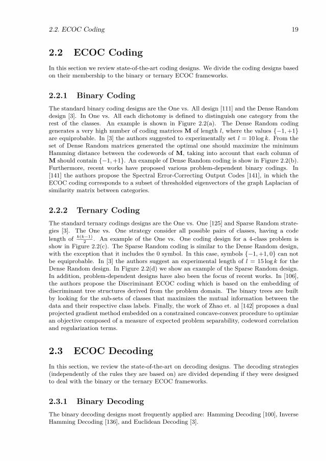
2 Error-Correcting Output Codes review and properties 172.1 The Error-Correcting Output Codes Framework . . . . . . . . . . . . . . . . . 172.2 ECOC Coding . . . . . . . . . . . . . . . . . . . . . . . . . . . . . . . . . . . 19

2.2.1 Binary Coding . . . . . . . . . . . . . . . . . . . . . . . . . . . . . . . 192.2.2 Ternary Coding . . . . . . . . . . . . . . . . . . . . . . . . . . . . . . . 19

2.3 ECOC Decoding . . . . . . . . . . . . . . . . . . . . . . . . . . . . . . . . . . 192.3.1 Binary Decoding . . . . . . . . . . . . . . . . . . . . . . . . . . . . . . 192.3.2 Ternary Decoding . . . . . . . . . . . . . . . . . . . . . . . . . . . . . 21

2.4 Good practices in ECOC . . . . . . . . . . . . . . . . . . . . . . . . . . . . . . 212.5 ECOC constraints . . . . . . . . . . . . . . . . . . . . . . . . . . . . . . . . . 222.6 Conclusions . . . . . . . . . . . . . . . . . . . . . . . . . . . . . . . . . . . . . 23

3 A novel representation for ECOCs: the Separability Matrix 253.1 The Separability matrix . . . . . . . . . . . . . . . . . . . . . . . . . . . . . . 253.2 From global to pair-wise correction capability . . . . . . . . . . . . . . . . . . 253.3 Conclusions . . . . . . . . . . . . . . . . . . . . . . . . . . . . . . . . . . . . . 26

II Learning ECOC representations 29

4 Learning ECOCs using Genetic Algorithms 314.1 Towards Reducing the ECOC Code Length . . . . . . . . . . . . . . . . . . . 31

ix

x CONTENTS

4.2 Learning Minimal ECOCs using standard Genetic Algorithms . . . . . . . . . 334.2.1 Minimal ECOC Coding . . . . . . . . . . . . . . . . . . . . . . . . . . 334.2.2 Evolutionary Minimal ECOC Learning . . . . . . . . . . . . . . . . . . 344.2.3 Experiments . . . . . . . . . . . . . . . . . . . . . . . . . . . . . . . . 37

4.3 Learning ECOCs using ECOC-compliant Genetic Algorithms . . . . . . . . . 424.3.1 Genetic Algorithms in the ECOC Framework . . . . . . . . . . . . . . 424.3.2 ECOC-Compliant Genetic Algorithm . . . . . . . . . . . . . . . . . . . 434.3.3 Experiments . . . . . . . . . . . . . . . . . . . . . . . . . . . . . . . . 524.3.4 Discussion . . . . . . . . . . . . . . . . . . . . . . . . . . . . . . . . . . 56

4.4 Conclusions . . . . . . . . . . . . . . . . . . . . . . . . . . . . . . . . . . . . . 60

5 Learning ECOCs via the Error-Correcting Factorization 635.1 Error-Correcting Factorization . . . . . . . . . . . . . . . . . . . . . . . . . . 63

5.1.1 Objective . . . . . . . . . . . . . . . . . . . . . . . . . . . . . . . . . . 645.1.2 Optimization . . . . . . . . . . . . . . . . . . . . . . . . . . . . . . . . 645.1.3 Connections to Singular Value Decomposition, Nearest Correlation

Matrix and Discrete Basis problems . . . . . . . . . . . . . . . . . . . 655.1.4 Ensuring a representable design matrix . . . . . . . . . . . . . . . . . 665.1.5 Defining a code length with representation guarantees . . . . . . . . . 675.1.6 Order of Coordinate Updates . . . . . . . . . . . . . . . . . . . . . . . 685.1.7 Approximation Errors and Convergence results when D is an inner

product of binary data . . . . . . . . . . . . . . . . . . . . . . . . . . . 695.2 Experiments . . . . . . . . . . . . . . . . . . . . . . . . . . . . . . . . . . . . . 71

5.2.1 Data . . . . . . . . . . . . . . . . . . . . . . . . . . . . . . . . . . . . . 715.2.2 Methods and settings . . . . . . . . . . . . . . . . . . . . . . . . . . . 715.2.3 Experimental Results . . . . . . . . . . . . . . . . . . . . . . . . . . . 72

5.3 Conclusions . . . . . . . . . . . . . . . . . . . . . . . . . . . . . . . . . . . . . 73

III Applications in Pose Estimation Problems 79

6 Applications of ECOCs in Pose Estimation Problems 816.1 Human Pose Estimation . . . . . . . . . . . . . . . . . . . . . . . . . . . . . . 816.2 HuPBA 8K+ Dataset . . . . . . . . . . . . . . . . . . . . . . . . . . . . . . . 836.3 ECOC and GraphCut based multi-limb segmentation . . . . . . . . . . . . . . 84

6.3.1 Body part learning using cascade of classifiers . . . . . . . . . . . . . . 846.3.2 Tree-structure learning of human limbs . . . . . . . . . . . . . . . . . 846.3.3 ECOC multi-limb detection . . . . . . . . . . . . . . . . . . . . . . . . 856.3.4 Binary GraphCut optimization for foreground mask extraction . . . . 866.3.5 Tree-structure body part learning without background . . . . . . . . . 866.3.6 ECOC multi-limb detection . . . . . . . . . . . . . . . . . . . . . . . . 866.3.7 Alpha-beta swap Graph Cuts multi-limb segmentation . . . . . . . . . 87

6.4 Experimental results . . . . . . . . . . . . . . . . . . . . . . . . . . . . . . . . 876.4.1 Data . . . . . . . . . . . . . . . . . . . . . . . . . . . . . . . . . . . . . 876.4.2 Methods and experimental settings . . . . . . . . . . . . . . . . . . . . 886.4.3 Validation measurement . . . . . . . . . . . . . . . . . . . . . . . . . . 886.4.4 Multi-limb segmentation results . . . . . . . . . . . . . . . . . . . . . . 88

6.5 Conclusions . . . . . . . . . . . . . . . . . . . . . . . . . . . . . . . . . . . . . 89

CONTENTS xi

IV Epilogue 97

7 Conclusions 997.1 Summary of contributions . . . . . . . . . . . . . . . . . . . . . . . . . . . . . 997.2 Future work . . . . . . . . . . . . . . . . . . . . . . . . . . . . . . . . . . . . . 100

A Datasets 101

B Publications 105B.1 Journals . . . . . . . . . . . . . . . . . . . . . . . . . . . . . . . . . . . . . . . 105B.2 International Conferences and Workshops . . . . . . . . . . . . . . . . . . . . 105

xii CONTENTS

List of Figures

1.1 Baby analyzing shapes and colors. . . . . . . . . . . . . . . . . . . . . . . . . 11.2 Chair samples. . . . . . . . . . . . . . . . . . . . . . . . . . . . . . . . . . . . 41.3 Standard pipeline for statistical pattern recognition. . . . . . . . . . . . . . . 51.4 Nao detects and classifies the furniture in the scene. . . . . . . . . . . . . . . 6

2.1 (a) Feature space and trained boundaries of dichotomizers. (b) Coding matrixM, where black and white cells correspond to −1,+1, denoting the twopartitions to be learnt by each base classifier (white cells vs. black cells)while grey cells correspond to 0 (ignored classes). (c) Decoding step, wherethe predictions of classifiers, h1, . . . , h5 for sample xt are compared to thecodewords m1, . . . ,m5 and xt is labelled as the class codeword at minimumdistance. . . . . . . . . . . . . . . . . . . . . . . . . . . . . . . . . . . . . . . . 18

2.2 (a) ECOC One vs. All coding design. (b) Dense Random coding desing. (c)Sparse Random coding. (d) One vs. One ECOC coding design. . . . . . . . . 20

3.1 ECOC codings of One vs. All (a), Dense Random (b), Sparse Random (c) andOne vs. One (d). Separability matrices for One vs. All (e), Dense Random(f), Sparse Random (g) and One vs. One coding (h). Note how predefinedcoding designs generate constant separability matrices, while other designspresent different distributions of separation between codewords. . . . . . . . . 27

3.2 Example of global versus pair-wise correction capability. On the left side ofthe figure the calculation of the global correction capability is shown. Theright side of the image shows a sample of pair-wise correction calculation forcodewords m2 and m8. . . . . . . . . . . . . . . . . . . . . . . . . . . . . . . 28

4.1 Number of classifiers per coding design and number of classes. . . . . . . . . . 324.2 (a) Binary Minimal, (b) Gray Minimal, and (c) One vs. All ECOC coding

designs of a 8-class problem. . . . . . . . . . . . . . . . . . . . . . . . . . . . . 334.3 Nested evolutionary optimization process for 3-class toy problem. . . . . . . . 374.4 Number of SVs for each method on UCI datasets. . . . . . . . . . . . . . . . . 404.5 Number of SVs for each method on Computer Vision datasets. . . . . . . . . 414.6 Diagram of the ECOC-Compliant Genetic Algortihm. . . . . . . . . . . . . . 444.7 Crossover example for a 5-class toy problem. (a) Feature space and trained

classifiers for parent IM . (b) ECOC coding matrix of parent IM . (c) Featurerepresentation and boundaries for parent IF . (d) Coding matrix of IF . (e)ECOC coding matrix composition steps for the offspring IS . (f) Feature spaceand inherited classifiers for IS . . . . . . . . . . . . . . . . . . . . . . . . . . . 48

xiii

xiv LIST OF FIGURES

4.8 Mutation example for a 5-class toy problem. (a) Feature space and traineddichotomizers for and individual IT . (b) ECOC coding matrix of IT . (c)Confusion matrix of IT . (d) Mutated coding matrix. (e) Mutated featurespace with trained dichotomizers. . . . . . . . . . . . . . . . . . . . . . . . . . 51

4.9 Sparsity extension example for a 5-class toy problem. (a) Feature space andtrained dichotomizers for IT . (b) ECOC coding matrix of IT . (c) Confusionmatrix of IT . (d) Extended coding matrix. (e) Extended feature space withtrained dichotomizers. . . . . . . . . . . . . . . . . . . . . . . . . . . . . . . . 53

4.10 Critical difference for the Nemenyi test and the performance per classifierranking values. . . . . . . . . . . . . . . . . . . . . . . . . . . . . . . . . . . . 55

4.11 (a) Number of classifiers per λ value on the UCI Vowel dataset. (b) Numberof SVs per coding design in the Computer Vision problems. . . . . . . . . . . 58

4.12 Number of SVs per coding design in the UCI datasets. . . . . . . . . . . . . . 594.13 (a) Classification error evolution for the Glass dataset. (b) Evolution of the

Performance per classifier rate for the Glass dataset. (c)Classification errorevolution for the Vowel dataset.(d) Evolution of the Performance per classifierrate for the Vowel dataset. (e)Classification error evolution for the Yeastdataset. (f) Evolution of the Performance per classifier rate for the Yeastdataset. . . . . . . . . . . . . . . . . . . . . . . . . . . . . . . . . . . . . . . . 60

5.1 D matrix for the Traffic (a) and ARFace (b) datasets. MM> term obtainedvia ECF for Traffic (c) and ARFace (d) datasets. ECOC coding matrix Mobtained with ECF for Traffic (e) and ARFace (f). . . . . . . . . . . . . . . . 68

5.2 Mean Frobenius norm value with standard deviation as a function of thenumber of coordinate updates on 50 different trials. The blue shaded areacorresponds to cyclic update while the red area denotes random coordinateupdates for Vowel (a) and ARFAce (b) datasets. . . . . . . . . . . . . . . . . 69

5.3 (Mean objective value and standard deviation for 30 runs of ECF on a randomDG of 10 classes (a), 100 classes (b), and 500 classes (c). (d) Toy problemsynthetic data, where each color corresponds to a different category in themulti-class problem. . . . . . . . . . . . . . . . . . . . . . . . . . . . . . . . . 70

5.4 Toy problem synthetic data, where each color corresponds to a different cat-egory in the multi-class problem. . . . . . . . . . . . . . . . . . . . . . . . . . 71

5.5 Multi-class classification accuracy (y axis) as a function of the relative com-putational complexity (x axis) for all datasets and both decoding measures. . 74

5.6 Multi-class classification accuracy (y axis) as a function of the number ofdichotomies for all datasets and both decoding measures (x axis). . . . . . . . 75

5.7 (a) Summary of performance of ECF-H method over all datasets using thenumber of SVs and the number of dichotomies as the measure of complexity,respectively for ECF-H (a)(d), ECF-E (b)(e) and OVA (c)(f). . . . . . . . . . 76

6.1 Different samples labeled on the HuPBA 8k+ dataset. . . . . . . . . . . . . . 906.2 Scheme of the proposed human-limb segmentation method. . . . . . . . . . . 916.3 (a) Tree-structure classifier of body parts, where nodes represent the defined dichotomies.

Notice that the single or double lines indicate the meta-class defined. (b) ECOC decodingstep, in which a head sample is classified. The coding matrix codifies the tree-structureof (a), where black and white positions are codified as +1 and −1, respectively. . . . . 92

6.4 Multi-limb segmentation results for the three methods, for each sample, wealso show the RGB image and the ground-truth (GT). . . . . . . . . . . . . . 93

LIST OF FIGURES xv

6.5 Multi-limb segmentation results for the three methods, for each sample, wealso show the RGB image and the ground-truth (GT). . . . . . . . . . . . . . 94

6.6 Jaccard Indexes for the different limb categories from (a) to (f). (g) MeanJaccard Index among all limb categories. . . . . . . . . . . . . . . . . . . . . . 95

A.1 Labeled Faces in the Wild dataset. . . . . . . . . . . . . . . . . . . . . . . . . 102A.2 Traffic sign classes. . . . . . . . . . . . . . . . . . . . . . . . . . . . . . . . . . 102A.3 ARFaces dataset classes. Examples from a category with neutral, smile, anger,

scream expressions, wearing sun glasses, wearing sunglasses and left light on,wearing sun glasses and right light on, wearing scarf, wearing scarf and leftlight on, and wearing scarf and right light on. . . . . . . . . . . . . . . . . . 103

A.4 (a) Object samples. (b) Old music score. . . . . . . . . . . . . . . . . . . . . . 104A.5 MPEG7 samples. . . . . . . . . . . . . . . . . . . . . . . . . . . . . . . . . . . 104

xvi LIST OF FIGURES

List of Tables

1.1 Summary of classification methods. . . . . . . . . . . . . . . . . . . . . . . . . 91.2 Table of symbols. . . . . . . . . . . . . . . . . . . . . . . . . . . . . . . . . . . 14

4.1 Classification results and number of classifiers per coding design. . . . . . . . 384.2 Classification results and number of classifiers per coding design. . . . . . . . 564.3 Mean rank per coding design. . . . . . . . . . . . . . . . . . . . . . . . . . . . 57

5.1 Percentage of wins over all datasets for each method using as a complexitymeasure the number SVs and the number of classifiers. Last row shows theaverage complexity of each method over all datasets. Abbreviations: ECF-H(H), ECF-E (E), OVA (A), OVO (O), DENSE (D), RAND (R), S-ECOC(S). 73

6.1 Comparison of public dataset characteristics. . . . . . . . . . . . . . . . . . . 836.2 Prior cost between each pair of labels. . . . . . . . . . . . . . . . . . . . . . . 87

A.1 UCI repository datasets characteristics. . . . . . . . . . . . . . . . . . . . . . 101

xvii

xviii LIST OF TABLES

Chapter 1

Introduction

The quintessential goal of Artificial Intelligence is to build systems that replicate (or evenimprove) the processes performed by humans in order to acquire knowledge and interpretthe environment around them. Although the Artificial Intelligence field has recently seenenormous advances, specially in those areas regarding with acquisition of knowledge fromperception (e.g Computer Vision, Speech Recognition, Remote Sensing, etc.), we are still farfrom reaching human performance in different tasks.

This is due to the fact that humans spend an incredible number of hours gatheringinformation from which make hypotheses, which become more credible as the quantity ofinformation acquired increases. This phenomenon is clearly observed in babies (see Figure1.1), which spend few years perceiving their environment by looking, touching, hearing,smelling and asking an innumerable number of questions. This acquisition of informationby means of the sensory stimuli and supervision, leads to an improvement on the confidenceof their hypotheses. This process is referred to as learning. In fact, the problem of takingdecisions among different hypotheses given sensory stimuli is often described as supervisedcategorization.

This dissertation tackles the problem of modeling different hypotheses to solve multi-classpattern and object categorization problems.

Figure 1.1: Baby analyzing shapes and colors.

1

2 INTRODUCTION

1.1 MotivationHumans perceive and reason about the world that surrounds them from multi-modal stimulithat sensory organs capture. Even though those stimuli are of different nature and thereforecome from different sensory organs (e.g. light stimuli is captured by the retina in our eyeswhile sound waves are captured by the cochlea in our ears), the brain is able to process andintegrate all this information. The mammalian brain has been studied over years, yieldinginteresting findings on its topological organization. As a result, it has been observed thatthe cerebral cortex can be categorized in three kinds of regions:

• Motor areas, which are dedicated to move parts of the body.• Sensory areas, dedicated to process the input signals captured by sensory organs. For

example, the V1 area (primary visual cortex) is specialized in recognizing patternscoming from visual stimuli, while the A1 area (primary auditory cortex) is specializedin processing sounds captured by the ears. In addition, some smaller regions have beendiscovered to be dedicated to much specific tasks, e.g. the Fusiform Face Area [78] forfacial recognition, the Parahippocampal Place Area [44] for scene context recognition,or the Extrastriate Body Area [40] for recognizing parts of the human body.

• Association areas, produce meaningful perceptual experience of the world by integrat-ing sensory information and information stored in memory. As pointed out by [140],association areas are globally organized as distributed networks, connecting differentwidely-spaced parts of the human brain. More specifically, the authors found a coarseparcellation of the brain in seven different regions (and a finer categorization in 17 re-gions), which can be connected following different pathways. While it is clear that ourbrains integrate signals and hypotheses coming from different sensory modalities, forexample, when trying to perform recognition a word from its sound and the move-ment of the lips of the speaker, it still remains unclear how this integration processis exactly performed. Among the different theories, statistical integration has beenbacked by a number or works providing results that correlate with human behaviour[13, 92, 134].

Given that different sensory modalities are not equally reliable (e.g. vision is usuallymore reliable than hearing in daylight, but not at night), it is natural to think of a statisticalapproach or a combination of statistical approaches to combine multi-modal cues comingfrom different senses. Hence, it has been shown that in order to improve the confidence ofthe decision making process the human brain uses information coming from different sensoryareas in the brain [140]. This has three obvious reasons:

• The decision taking capabilities of the brain, although great are limited and can bedefective in certain situations.

• The information acquired by the sensory areas in the brain can be imperfect, due toenvironmental conditions or faulty processing abilities.

• The experience stored in memory only represents a part of the space of the informationand possible decisions available for the task.

Therefore, by using different sources of information the brain is able to make moreconfident decisions with a capability to generalize to different tasks.

However, studies have shown that the reasoning processes related to our visual systemplay a very important role in our global intelligent behavior. This can be often proved bytrying to interact with our daily environment without perceiving visual information. Beingdeprived of this information makes simple tasks (i.e walking, avoiding obstacles, etc.) much

1.2. Statistical Pattern Recognition 3

harder. The area of Artificial Intelligence that deals with the processing of visual informationis known as Computer Vision, and it covers from the extraction valuable information fromdigital two-dimensional projections of the real world, up to how process that informationto obtain high level representations to understand and make sense of what is happening inthose images.

For this reason, in this dissertation we are particularly interested in categorization prob-lems which deal with visual data as their main source of information.

1.2 Statistical Pattern RecognitionAutomatic (machine) recognition, description, classification, and grouping of patterns areimportant problems in a variety of engineering and scientific disciplines such as biology,psychology, medicine, marketing, computer vision, artificial intelligence, and remote sensing.But what is a pattern? Watanabe [132] defines a pattern as the opposite of chaos; it isan entity, that could be given a name and which exhibits a certain type of structure. Forexample, a pattern could be a fingerprint image, a handwritten cursive word, a human face,or a speech signal. Given a pattern, its recognition/classification may consist of one ofthe following tasks: 1) Supervised Classification (categorization) in which the input patternis identified as a member of a predefined class, 2) Unsupervised Classification (clustering)in which the pattern is assigned to a hitherto unknown class. Note that the recognitionproblem here is being posed as a classification or categorization task, where the classes areeither defined by the system designer (categorization) or are learned based on the similarityof patterns (clustering). 3) Semi-supervised learning is halfway between supervised andunsupervised learning. In addition to patters without any predefined classes, the algorithmis also provided with some patterns with their predefined classes – but not necessarily for allexamples.

Statistical Pattern Recognition denotes as Supervised Classification the problem ofmaking a decision based on certain learning information available. [76]. In this sense, aclassification system looks for a method that makes those judgments or decisions in previouslyunseen situations. In particular, a binary classification task refers to the problem of makinga decision for a new object xi (data sample or pattern), so that ξi is classified among twopredefined categories (or classes), c1 and c2. Thus, in binary classification we only havetwo alternatives to decide amongst c1 and c2. Formally, given training data X,y X ∈Rn×m,y ∈ c1, c21×n, where xi is the i−th object and yi is the true class of object xi, aclassifier function f is trained to distinguish the objects which label is c1 from the objectswhich label is c2. The classifier function is defined as f : X → y, where yi ∈ c1, c2∀i ∈1, . . . , n. However, in order to approximate or learn the classifier f each element xi shouldbe described with a set of characteristic or features, inherent to the object itself. For instance,we could describe a baby based on his weight, height, eyes color, etc. Then, the process ofapproximating the classifier function also called learning or training uses the set of objectfeatures from all the samples in order to define a boundary between two classes.

There are different techniques that deal with the task of object/pattern description[14][91]. Informative features depends on the object itself and its relationships with otherclasses, as well as the problem one wants to solve. In addition, some features can changetheir description when environmental factors introduce noise in the description process. Forexample, using the weight as feature description of a baby can be sensible to the planet inwhich this measure is being performed. In particular, when describing or extracting featuresfrom images, we can find that such features are sensible to changes in illumination, occlusionsbetween parts or deformations on non-rigid entities.

4 INTRODUCTION

The problem of object description is a very difficult task. Observe the objects of Figure1.2. Which are the representative features to describe a chair? shape? color? Obviously, itdepends on the categorization problem we consider. Binary classification not only does con-sist on distinguishing apples from tables. In the chair class, we can also apply categorization.Which chairs are broken? Which chairs are black or brown? These questions correspond tobinary problems. In the first case, the variations of the shape of the object can be useful,but not the color. In the second case, the color has an outstanding decision, while the shapeis not a relevant feature.

Figure 1.2: Chair samples.

Given the features or descriptions obtained for each data sample, in the statistical ap-proach, each of these patterns is viewed as a point in a high-dimensional space of features.Then, the goal is to choose those features that allow pattern vectors belonging to differentcategories to occupy compact and disjoint regions in that feature space [17]. The effectivenessof the representation space (feature set) is determined by how well patterns from differentclasses can be separated. Given a set of training patterns from each class, the objective isto establish decision boundaries in the feature space which separate patterns belonging todifferent classes. In the statistical decision theoretic approach, the decision boundaries aredetermined by the probability distributions of the patterns belonging to each class, whichmust either be specified or learnt [17][129].

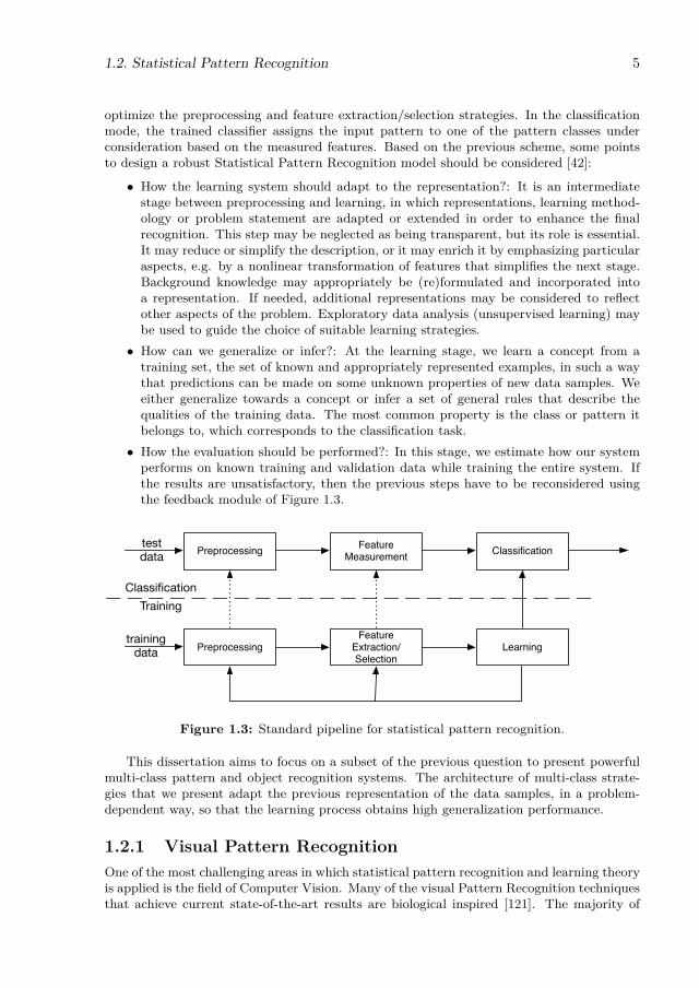
The classification or categorization system is operated in two modes: learning (training)and classification (testing) (see Figure 1.3). The role of the preprocessing module is to re-move noise, normalize the pattern, and any other operation which will contribute in defininga compact representation of the data samples. In the training mode, the feature extrac-tion/selection module finds the appropriate features for representing the input patterns andthe classifier is trained to partition the feature space. The feedback path allows a designer to

1.2. Statistical Pattern Recognition 5

optimize the preprocessing and feature extraction/selection strategies. In the classificationmode, the trained classifier assigns the input pattern to one of the pattern classes underconsideration based on the measured features. Based on the previous scheme, some pointsto design a robust Statistical Pattern Recognition model should be considered [42]:

• How the learning system should adapt to the representation?: It is an intermediatestage between preprocessing and learning, in which representations, learning method-ology or problem statement are adapted or extended in order to enhance the finalrecognition. This step may be neglected as being transparent, but its role is essential.It may reduce or simplify the description, or it may enrich it by emphasizing particularaspects, e.g. by a nonlinear transformation of features that simplifies the next stage.Background knowledge may appropriately be (re)formulated and incorporated intoa representation. If needed, additional representations may be considered to reflectother aspects of the problem. Exploratory data analysis (unsupervised learning) maybe used to guide the choice of suitable learning strategies.

• How can we generalize or infer?: At the learning stage, we learn a concept from atraining set, the set of known and appropriately represented examples, in such a waythat predictions can be made on some unknown properties of new data samples. Weeither generalize towards a concept or infer a set of general rules that describe thequalities of the training data. The most common property is the class or pattern itbelongs to, which corresponds to the classification task.

• How the evaluation should be performed?: In this stage, we estimate how our systemperforms on known training and validation data while training the entire system. Ifthe results are unsatisfactory, then the previous steps have to be reconsidered usingthe feedback module of Figure 1.3.

PreprocessingFeature

Measurement Classification

PreprocessingFeature

Extraction/Selection

Learning

Classification

Training

training data

testdata

Figure 1.3: Standard pipeline for statistical pattern recognition.

This dissertation aims to focus on a subset of the previous question to present powerfulmulti-class pattern and object recognition systems. The architecture of multi-class strate-gies that we present adapt the previous representation of the data samples, in a problem-dependent way, so that the learning process obtains high generalization performance.

1.2.1 Visual Pattern RecognitionOne of the most challenging areas in which statistical pattern recognition and learning theoryis applied is the field of Computer Vision. Many of the visual Pattern Recognition techniquesthat achieve current state-of-the-art results are biological inspired [121]. The majority of

6 INTRODUCTION

studies in this area assume that not all parts of an image give us valuable information,and only analyzing the most important parts of the image in detail is sufficient to performrecognition or categorization tasks. The biological structure of the eye is such that a highresolution fovea and its low-resolution periphery provide data for recognition purposes. Thefovea is not static, but is moved around the visual field in facades. These sharp, directedmovements of the fovea are not random. The periphery provides low-resolution information,which is processed to reveal salient points as targets for the fovea, and those are inspectedwith the fovea. The eye movements are a part of overt attention, as opposed to covertattention which is the process of moving an attentional focus around the perceived imagewithout moving the eye. In the case of Neural Networks, the objective is to simulate thebehavior of some neuronal circuits of our brain.

To model a Visual Pattern Recognition problem, a common approach consists of detectingthe objects in an image, and then, classifying them to their respective category. Manyrecognition systems also treat the problem of object detection as a binary classificationproblem, where the information of each part of the image is classified as object or background.Look to the situation presented in 1.4.

?

Figure 1.4: Nao detects and classifies the furniture in the scene.

The humanoid robot Nao from Aldebaran Robotics captures images from a scene, dis-carding background regions. At the first step, it treats to find the regions of the imagethat contain a piece of furniture. Once the region containing a piece of furniture is found,given four previous furniture categories, Nao classifies the inner object as a chair. Hence,the problem of object recognition can be seen as an object detection problem followed by aclassification procedure.

1.3 The Multi-class Classification ProblemWhen using the term binary classification, the labels from classes c1 and c2 use to take thevalues +1 or −1, respectively as a convention. At the learning process explained in previoussections, the labels for the training objects are known.

1.4. State-of-the-art Classification Techniques in Visual Pattern Recognition 7

In previous examples, the underlaying problem corresponded to Supervised Binary Clas-sification. However, Binary Classification is far from representing real world problems. Wecan classify between black and brown chairs or we can also distinguish among chairs, tables,couches, lamps, etc. Multi-class classification is the term applied to those Machine Learningproblems that require assigning labels to instances where the labels are drawn from a setof at least three classes. Real-world situations are full of multi-class classification problems,where we want to distinguish among k possible categories (obviously, the number of objectsthat we have learnt during our life tends to be uncountable). If we can design a multi-classifier F , then the prediction can be understood as in the binary classification problem,being F : X → y, where now yi ∈ 1, . . . , k, for a k−class problem. Several multi-classclassification strategies have been proposed in the literature. However, though there arevery powerful binary classifiers, many strategies fail to manage multi-class information. Aswe show in successive sections, a possible multi-class solution could potentially consist ofdesigning and combining of a set of binary classification problems.

1.4 State-of-the-art Classification Techniques in Vi-sual Pattern Recognition

In this chapter we describe the state-of-the-art techniques for classification with a particularinterest in those applied in Computer Vision.

1.4.1 ClassifiersIn the Statistical Pattern Recognition field, classifiers are frequently grouped into those basedon similarities, probabilities, or geometric information about class distribution [41, 76].

1. Similarity Maximization Methods: The Similarity Maximization Methods use the sim-ilarity between patterns to decide a classification. The main issue in this type ofclassifiers is the definition of the similarity measure.

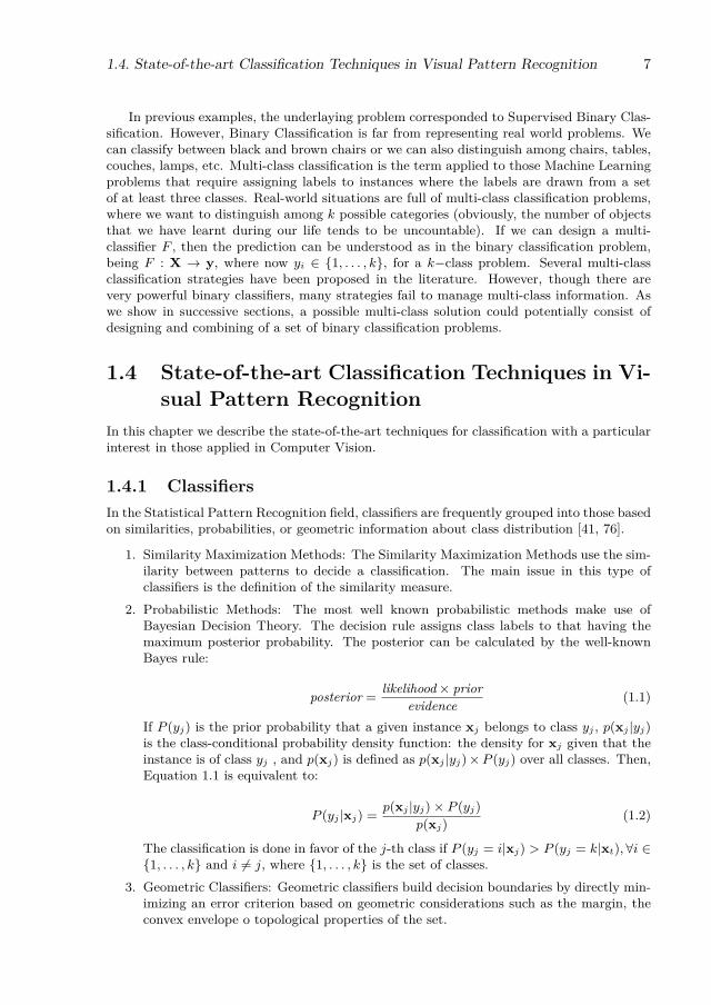
2. Probabilistic Methods: The most well known probabilistic methods make use ofBayesian Decision Theory. The decision rule assigns class labels to that having themaximum posterior probability. The posterior can be calculated by the well-knownBayes rule:

posterior = likelihood× priorevidence (1.1)

If P (yj) is the prior probability that a given instance xj belongs to class yj , p(xj |yj)is the class-conditional probability density function: the density for xj given that theinstance is of class yj , and p(xj) is defined as p(xj |yj)×P (yj) over all classes. Then,Equation 1.1 is equivalent to:

P (yj |xj) = p(xj |yj)× P (yj)p(xj)

(1.2)

The classification is done in favor of the j-th class if P (yj = i|xj) > P (yj = k|xt), ∀i ∈1, . . . , k and i 6= j, where 1, . . . , k is the set of classes.

3. Geometric Classifiers: Geometric classifiers build decision boundaries by directly min-imizing an error criterion based on geometric considerations such as the margin, theconvex envelope o topological properties of the set.

8 INTRODUCTION

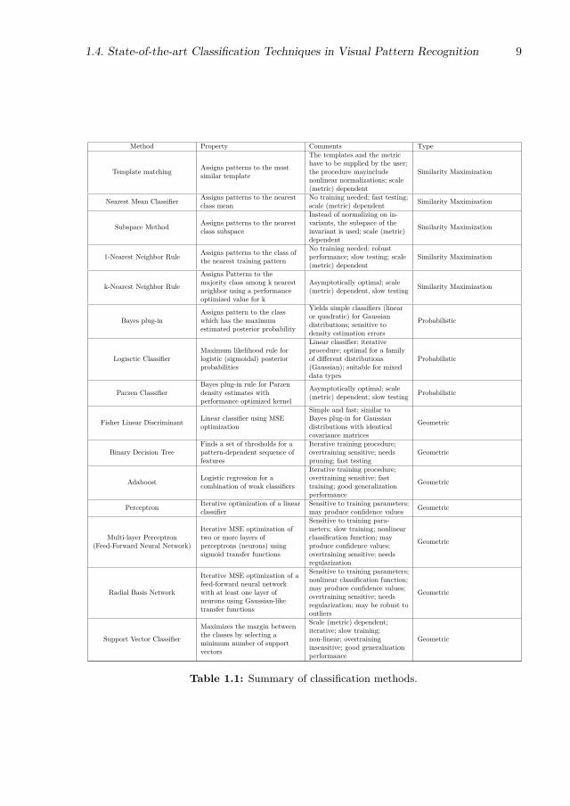
Table 1.1 summarizes the main classification strategies studied in literature. For eachstrategy, we show its properties, comments, and type based on the previous grouping.

1.4.2 Multi-class classifiers

Intrinsic multi-class methods

In classification problems the goal is to find a function F : X → y, where X is the setof observations and y ∈ 1, . . . , k1×n the set composed by the label of each observation(max(y) > 2 for the multi-class context). The goal of F is to map each observation xi ∈R1×m to its label yi ∈ 1, . . . , k. There are many possible strategies for estimating F ,nevertheless, literature has shown that the complexity for estimating a unique F for thewhole multi-class problem grows with the cardinality of the label set. In this sense, mostof the strategies aim to model the probability density function of each category. Moreover,lazy learning methods like Nearest Neighbours to estimate k by a local search of the mostproximate observations.

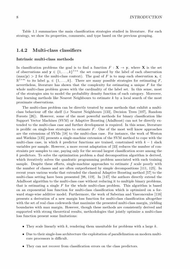
The multi-class problem can be directly treated by some methods that exhibit a multi-class behaviour off the shelf (i.e Nearest Neighbours [133], Decision Trees [107], RandomForests [26]). However, some of the most powerful methods for binary classification likeSupport Vector Machines (SVM) or Adaptive Boosting (AdaBoost) can not be directly ex-tended to the multi-class case and further development is required. In this sense, literatureis prolific on single-loss strategies to estimate F . One of the most well know approachesare the extensions of SVMs [18] to the multi-class case. For instance, the work of Westonand Watkins [135] presents a single-machine extension of the SVM method to cope with themulti-class case, in which k predictor functions are trained, constrained with k − 1 slackvariables per sample. However, a more recent adaptation of [33] reduces the number of con-straints per samples to one, paying only for the second largest classification score among thek predictors. To solve the optimization problem a dual decomposition algorithm is derived,which iteratively solves the quadratic programming problem associated with each trainingsample. Despite these efforts, single-machine approaches to estimate f scale poorly withthe number of classes and are often outperformed by simple decompositions [111, 125]. Inrecent years various works that extended the classical Adaptive Boosting method [57] to themulti-class setting have been presented [98, 119]. In [147] the authors directly extend theAdaBoost algorithm to the multi-class case without reducing it to multiple binary problems,that is estimating a single F for the whole multi-class problem. This algorithm is basedon an exponential loss function for multi-class classification which is optimized on a for-ward stage-wise additive model. Furthermore, the work of Saberian and Vasconcenlos [116]presents a derivation of a new margin loss function for multi-class classification altogetherwith the set of real class codewords that maximize the presented multi-class margin, yieldingboundaries with max margin. However, though these methods are consistently derived andsupported with strong theoretical results, methodologies that jointly optimize a multi-classloss function present some limitations:

• They scale linearly with k, rendering them unsuitable for problems with a large k.

• Due to their single-loss architecture the exploitation of parallelization on modern multi-core processors is difficult.

• They can not recover from classification errors on the class predictors.

1.4. State-of-the-art Classification Techniques in Visual Pattern Recognition 9

Method Property Comments Type

Template matching Assigns patterns to the mostsimilar template

The templates and the metrichave to be supplied by the user;the procedure mayincludenonlinear normalizations; scale(metric) dependent

Similarity Maximization

Nearest Mean Classifier Assigns patterns to the nearestclass mean

No training needed; fast testing;scale (metric) dependent Similarity Maximization

Subspace Method Assigns patterns to the nearestclass subspace

Instead of normalizing on in-variants, the subspace of theinvariant is used; scale (metric)dependent

Similarity Maximization

1-Nearest Neighbor Rule Assigns patterns to the class ofthe nearest training pattern

No training needed; robustperformance; slow testing; scale(metric) dependent

Similarity Maximization

k-Nearest Neighbor Rule

Assigns Patterns to themajority class among k nearestneighbor using a performanceoptimized value for k

Asymptotically optimal; scale(metric) dependent, slow testing Similarity Maximization

Bayes plug-inAssigns pattern to the classwhich has the maximumestimated posterior probability

Yields simple classifiers (linearor quadratic) for Gaussiandistributions; sensitive todensity estimation errors

Probabilistic

Logisctic ClassifierMaximum likelihood rule forlogistic (sigmoidal) posteriorprobabilities

Linear classifier; iterativeprocedure; optimal for a familyof different distributions(Gaussian); suitable for mixeddata types

Probabilistic

Parzen ClassifierBayes plug-in rule for Parzendensity estimates withperformance optimized kernel

Asymptotically optimal; scale(metric) dependent; slow testing Probabilistic

Fisher Linear Discriminant Linear classifier using MSEoptimization

Simple and fast; similar toBayes plug-in for Gaussiandistributions with identicalcovariance matrices

Geometric

Binary Decision TreeFinds a set of thresholds for apattern-dependent sequence offeatures

Iterative training procedure;overtraining sensitive; needspruning; fast testing

Geometric

Adaboost Logistic regression for acombination of weak classifiers

Iterative training procedure;overtraining sensitive; fasttraining; good generalizationperformance

Geometric

Perceptron Iterative optimization of a linearclassifier

Sensitive to training parameters;may produce confidence values Geometric

Multi-layer Perceptron(Feed-Forward Neural Network)

Iterative MSE optimization oftwo or more layers ofperceptrons (neurons) usingsigmoid transfer functions

Sensitive to training para-meters; slow training; nonlinearclassification function; mayproduce confidence values;overtraining sensitive; needsregularization

Geometric

Radial Basis Network

Iterative MSE optimization of afeed-forward neural networkwith at least one layer ofneurons using Gaussian-liketransfer functions

Sensitive to training parameters;nonlinear classification function;may produce confidence values;overtraining sensitive; needsregularization; may be robust tooutliers

Geometric

Support Vector Classifier

Maximizes the margin betweenthe classes by selecting aminimum number of supportvectors

Scale (metric) dependent;iterative; slow training;non-linear; overtraininginsensitive; good generalizationperformance

Geometric

Table 1.1: Summary of classification methods.

10 INTRODUCTION

Ensemble Learning for multi-class problemsMulti-class classification (i.e. automatically attributing a label to each sample of the dataset)is one of the classic problems in Pattern Recognition and Machine Intelligence. In this sec-tion we review the state-of-the-art for Ensemble Learning techniques that tackle multi-classclassification problems.

Divide and Conquer ApproachesThe divide and conquer approach has drawn a lot of attention due to its excellent results

and easily parallelizable architecture [3, 7, 51, 64, 94, 106, 111, 125]. In this sense, insteadof developing a method to cope with the multi-class case, divide and conquer approachesdecouple F into a set of l binary problems which are treated separately F = f1, . . . , f l.Once the responses of binary classifiers are obtained a committee strategy is used to findthe final output. In this trend one can find three main lines of research: flat strategies,hierarchical classification, and ECOC. Flat strategies like One vs. One [125] and One vs.All [111] are those that use a predefined problem partition scheme followed by a committeestrategy to aggregate the binary classifier outputs. Hierarchical classification relies on asimilarity metric distance among classes to build a binary tree in which nodes correspondto different problem partitions [60, 64, 94]. Finally, the ECOC framework consists of twosteps: In the coding step, a set of binary partitions of the original problem are encoded ina matrix of discrete codewords [39] (univocally defined, one codeword per class). At thedecoding step a final decision is obtained by comparing the test codeword resulting of theunion of the binary classifier responses with every class codeword and choosing the classcodeword at minimum distance [47, 146]. The coding step has been widely studied in litera-ture, yielding three different types of codings: predefined codings [111, 125], random codings[3] and problem-dependent codings for ECOC [7, 51, 61, 106, 141, 142]. Predefined codingslike One vs. All or One vs. One are directly embeddable in the ECOC framework. In [3],the authors propose the Dense and Sparse Random coding designs with a fixed code lengthof 10, 15 log2(k), respectively. In [3] the authors encourage to generate a set of 104 ran-dom matrices and select the one that maximizes the minimum distance between rows, thusshowing the highest correction capability. However, the selection of a suitable code length lstill remains an open problem.

Problem-dependent designsAlternatively, problem-dependent strategies for ECOC have proven to be successful in

multi-class classification tasks [51, 60, 61, 106, 141, 142, 143, 144]. A common trend ofthese works is to exploit information of the multi-class data distribution obtained a prioriin order to design a decomposition into binary problems that are easily separable. In thatsense, [141] computes a spectral decomposition of the graph laplacian associated to themulti-class problem. The expected most separable partitions correspond to the thresholdedeigenvectors of the laplacian. However, this approach does not provide any warranties ondefining unequivocal codewords (which is a core property of the ECOC coding framework) orobtaining a suitable code length l. In [61], Gao and Koller propose a method which adaptivelylearns an ECOC coding by optimizing a novel multi-class hinge loss function sequentially.On an update of their earlier work, Gao and Koller propose in [60] a joint optimizationprocess to learn a hierarchy of classifiers in which each node corresponds to a binary sub-problem that is optimized to find easily separable subproblems. Nonetheless, although thehierarchical configuration speeds up the testing step, it is highly prone to error propagationsince node mis-classifications can not be recovered. In addition, the work of Zhao et. al[142] proposes a dual projected gradient method embedded on a constrained concave-convexprocedure to optimize an objective composed of a measure of expected problem separability,

1.4. State-of-the-art Classification Techniques in Visual Pattern Recognition 11

codeword correlation and regularization terms. In the light of these results, a general trendof recent works is to optimize a measure of binary problem separability in order to induceeasily separable sub-problems. This assumption leads to ECOC coding matrices that boostthe boundaries of easily separable classes while modeling with low redundancy the ones withmost confusion.

Furthermore, [10] proposed a standard Genetic Algorithm to optimize an ECOC ma-trix, known as Minimal ECOC matrix, which is the theoretical lower-bound in terms of thenumber of classifiers dlog2 k e. In this work the evaluation of each individual (ECOC ma-trix) is obtained by means of its classification error over the validation set. In addition, [62]proposed the use of the CHC Genetic Algorithm [52] to optimize a Sparse Random ECOCmatrix. In this work, the code length is fixed in the interval [30, 50] independently of thenumber of classes. Finally, [89] used a Genetic Algorithm to optimize a Sparse Randomcoding matrix of length in the interval [log2(k), k]. The evaluation of each individual (ECOCcoding matrix) is performed as the classification error over a validation set.

Convolutional Neural Networks

Neural Networks are a family of models inspired by biological neural networks. Thesemodels are generally presented as systems of interconnected "neurons" which exchange mes-sages between each other. The connections have numeric weights that can be tuned basedon training data, making neural nets adaptive to inputs and capable of learning. NeuralNetworks (NNs) were successfully applied to multi-class classification problem in 90s [123].These methods can be seen as a stacking of different neuron layers in which outputs of layeri are the input of layer i+ 1.

Particularly, the introduction of the multi-layer perceptron by Rosenblatt [113], whichwas demonstrated to be a universal function approximator [113] made Neural Networks ahot topic at the time. Furthermore, the introduction of back-propagation to train NeuralNetworks meant that these models could be trained efficiently [59, 113, 115]. However,with the appearance of SVMs in the mid 90s Neural Networks lost all there interest due tothe stronger theoretical properties and easier interpretation of the Support Vector Machinemodel.

In despite of the great performance exihibited by SVMs, several researchers kept onworking with Neural Networks after the introduction of SVMs [15, 16, 87, 121]. In thissense, based on previous work from Fukushima [59] Convolutional Neural Networks (CNNs)were first introduced by LeCun and Bengio [86]. The idea of this method was to use a setof convolutional layers to combine three architectural ideas to ensure some degree of shiftand distortion invariance: local receptive fields, shared weights and sometimes spatial ortemporal subsampling. Each neuron of a layer receives inputs from a set of units located ina small neighborhood in the previous layer.

However, it was not until the paper of Krizhevsky et. al [82] that Convolutional Neu-ral Networks gained an overwhelming attention given the fact that the method proposedby Krizhevsky et. al [82] outperformed other methods by 10% in the ILSRVC challenge[82]. This method followed the line of previous Convolutional Neural Networks [86], definin-ing a deep architecture with 5 convolutional layers and 3 fully-connected layers, generatinga model consisting of 60 million parameters. Convolutional Neural Networks have con-sistently outperformed state-of-the-art methods for most classification tasks in ComputerVision. However, further analyses of this methods on this dissertation falls out of scopegiven the overly large number of parameters and data needed to train these models.

12 INTRODUCTION

1.5 Objective of the ThesisIn this dissertation we are interested in proposing novel techniques to learn problem-dependentECOC coding designs for multi-class problems in Computer Vision, in particular, we are veryinterest in strategies that scale sub-linearly with the number of classes in the multi-class prob-lem. Hence, we most of our experimental results analyze performance as a function of thecomplexity of the model.

1. Reduce the code length of problem-dependent ECOC codings. Code lengthhas a direct implication in the model complexity of the overall ECOC model. Oneobjective of this dissertation is analyze and explore ECOC coding designs which codelength scales sub-linearly with the number of classes in the multi-class problem. There-fore rendering them suitable to treat problems with very large number of classes usingvery reduced computational resources.

2. Design strategies to optimize the ECOC coding designs. Another objective ofthis dissertation is to exploit the distribution of the multi-class data to define problem-dependent ECOC designs that distribute their learning effort accordingly. In order todo so, we study different ways of optimizing ECOC coding matrices.

3. Analyze and understand how error-correction is distributed among classes.Error-correction has always been in the core of all ECOC analyses. Our objective inthis dissertation is to show that the current way to analyze and understand error-correction for ECOC matrices does not reflect how the error-correction is distributedamong classes. Hence, a novel way of representing ECOCs and their correcting capa-bilities has to be defined.

1.6 ContributionsError-Correcting Output Codes were proposed to deal with multi-class problems by embed-ding several binary problems in a coding matrix. This approach showed to be very robustapplied to many real-world problems. However, several aspects of this framework that canhelp us to improve the classification performance have not been previously analyzed. In thisthesis, we theoretically and empirically analyze the ECOC framework.

1. Minimal ECOC Coding Design: We propose to define the lower bound of anECOC coding design in terms of the number of binary problems embedded in thecoding design. We show that even with a very reduced number of binary classifiers wecan obtain comparable results to state-of-the-art coding designs.

2. Genetic Optimization of Minimal ECOCs: Although showing a good perfor-mance, Minimal ECOCs are bounded in terms of generalization capabilities due tothe reduced number of classifiers. In this sense, we propose to use a Genetic Algo-rithm to optimize the ECOC coding configuration and obtain a Minimal ECOC codingmatrix with high generalization capabilities.

3. ECOC-Compliant Genetic Algorithm: Standard Genetic Algorithm use crossoverand mutation operators that treat individuals as binary strings. This operators do nottake into account the constraints of the ECOC framework and can lead to poor opti-mization schemes. We propose to redefine the standard crossover and mutation opera-tors in order to take into account the constraints of the ECOC framework. In additionwe also proposes and operator to dynamically adapt the code length of the ECOCduring the training process. This redefinition of operators leads to very satisfyingresults in terms of classification performance as a function of the model complexity.

1.7. Thesis Outline 13

4. ECOC separability and error-correction: The error-correcting capability of anECOC has always been depicted in literature as a single scalar, which hinders furtheranalyses of error-correction between different categories. We propose to represent anECOC by means of its separability matrix and use very simple heuristics to exploit thedistribution of error-correction among pairs of classes to outperform state-of-the-artresults.

5. Error-Correcting Factorization: Empowered by the novel representation of anECOC as its Separability Matrix we propose to obtain an estimated Separability ma-trix from data using very simple statistics. Then, we defined the novel Error-CorrectingFactorization to factorize that estimated Separability matrix into a discrete ECOCcoding matrix that distributes error-correcting to those classes that are more prone toerrors.

6. Applications in Human Pose Recovery: We applied the ECOC framework inthe challenging problem of Human Pose Recovery, obtaining very satisfying resultsin comparison with state-of-the-art works. In addition we propose the HuPBA 8k+dataset, a large dataset for Human Pose Recovery in still images.

The experimental results of this thesis show that the presented strategies outperformthe results of the state-of-the-art ECOC coding designs as well as the state-of-the-art multi-classifiers, being specially suitable to model several real multi-class categorization problems.

1.7 Thesis OutlineThis dissertation is organized as follows:

In Part I, Chapter 2 introduces the basis of the Error-Correcting Output Codes (ECOCs),as well as the state-of-the-art coding and decoding designs. In addition, we also present goodpractices for ECOC coding and the constraints of ECOC coding matrices. In Chapter 3 weintroduce a novel way to represent ECOCs by means of the separation between codewordsand analyze how error-correcting capabilities are distributed for state-of-the-art designs.

Part II presents our contributions to problem-dependent coding designs for ECOCs usingGenetic Algorithm in Chapter 4. In particular, we present the Minimal ECOC coding, whichdefines the lower bound in terms of the number of classifiers embedded in an ECOC codingmatrix. Moreover, we also present a novel Genetic Algorithm that takes into account theconstraints of the ECOC framework. Chapter 5 present a novel method to compute problem-dependent designs from ECOC based on the Error-Correcting Factorization, which factorizesan estimated codeword separability matrix obtained from training data.

In Part III Chapter 6 presents applications of ECOC codings in the challenging ComputerVision problem of Human Pose Estimation, in which we cast the problem of recognizing thehuman body parts as a classification problem at tackle it using the ECOC framework.

Finally, Part IV concludes the dissertation with a summary of contributions and futurework in Chapter 7. Annex A provided technical details of datasets used for experimentalresults, and Annex B shows the complete list of publications generated as a result of thisdissertation.

1.8 NotationWe introduce the notation for the this dissertation.

Bold capital letters denote matrices (e.g. X), bold lower-case letters represent vectors(e.g., x). All non-bold letters denote scalar variables. xi is the i−th row of the matrix X.

14 INTRODUCTION

xj is the j−th column of the matrix X. 1 is a matrix or vector of all ones of the appropriatesize. I is the identity matrix. diag(d) denotes a matrix with d in the main diagonal. xijdenotes the scalar in the i−th row and j−th column of X. ‖X‖F = tr(X>X) denotes theFrobenius norm. ‖·‖p is used to denote the Lp-norm. x⊕y is an operator which concatenatesvectors x and y . rank(X) denotes the rank of X. X ≤ 0 denotes the point-wise inequality.

Table 1.2 shows the different symbols used in this dissertation.

Matrix of training samples X i−th training sample xiVector of labels y label of the i−th samples yii-th category ci Indicator function I

ECOC coding matrix M i-th codeword mi

i−th dichotomy mi i−th classifier fiNumber of classes k Number of dichotomies l

Vector of classifier predictionsfor the i−th sample f(xi) Decoding measure δ

Chromosome s Error function E

Number of Generations G i−th individual IiConfusion matrix C Performance of binary classifiers p

Dichotomy selection order t Mutation control value mtcSeparability matrix H i-th row of H hi

Design Matrix D i−th row of D diMinimum distance between

pairs of codewords P i−th row of P pi

Matrix of eigenvectors V Vector of eigenvalues λLikelihood map B Weight matrix W

Table 1.2: Table of symbols.

Part I

Ensemble Learning and theECOC framework

15

Chapter 2

2.1 The Error-Correcting Output Codes FrameworkECOC is a general multi-class framework built on the basis error-correcting principles incommunication theory [39]. This framework suggests to view the task of supervised multi-class classification as a communication problem in which the label of a training example isbeing transmitted over a channel. The channel consists of the input features, the trainingexamples, and the learning algorithm. Because of errors introduced by the finite numberof training samples, choice of input features, and flaws in the learning process, the labelinformation is corrupted. By coding the label information in an error-correcting codewordand transmitting (i.e learning) each bit separately (i.e., via uncorrelated independent binaryclassifiers), the algorithm may be able to recover from the errors produced by the numberof samples, features or learning algorithm.

The ECOC framework is composed of two different steps: coding [3, 39] and decoding[47, 146]. At the coding step an ECOC coding matrix M ∈ −1,+1k×l is constructed, wherek denotes the number of classes in the problem and l the number of bi-partitions definedto discriminate the k classes. In this matrix, the rows (mi’s, also known as error-correctingcodewords or codewords for shorter) are univocally defined, since these are the identifiers ofeach category in the multi-class categorization problem. On the other hand, the columns ofM denote the set of bi-partitions, dichotomies, or meta-classes to be learnt by each binaryclassifier f (also known as dichotomizer). In this sense, classifier f j is responsible of learningthe bi-partition denoted on the j−th column of M. Therefore, each dichotomizer learns theclasses with value +1 against the classes with value −1 in a certain column. Note that theECOC framework is independent of the binary classifier applied. For notation purposes infurther sections we will refer to the entry of M at the i-th row and the j-th column as mij .Following this notation the i-th row (codeword of class ci) will be referred as mi and, thej-th column (j-th bi-partition or dichotomy) will be referred as mj .

Originally, the coding matrix was binary valued (M ∈ −1,+1k×l). However, [3] intro-duced a third value, and thus, M ∈ −1,+1, 0k×l, defining ternary valued coding matrices.In this case, for a given dichotomy categories can be valued as +1 or −1 depending on themeta-class they belong to, or 0 if they are ignored by the dichotomizer. This new value allowsthe inclusion of well-known decomposition techniques into the ECOC framework, such hasOne vs. One [125] or Sparse [3] decompositions.

At the decoding step a sample xt is classified among the k possible categories. In order toperform the classification task, each dichotomizer in f j predicts a binary value for xt whetherit belongs to one of the bi-partitions defined by the correspondent dichotomy. Once the setof predictions f(xt) ∈ Rl is obtained, it is compared to the codewords of M using a distance

17

18 ERROR-CORRECTING OUTPUT CODES REVIEW AND PROPERTIES

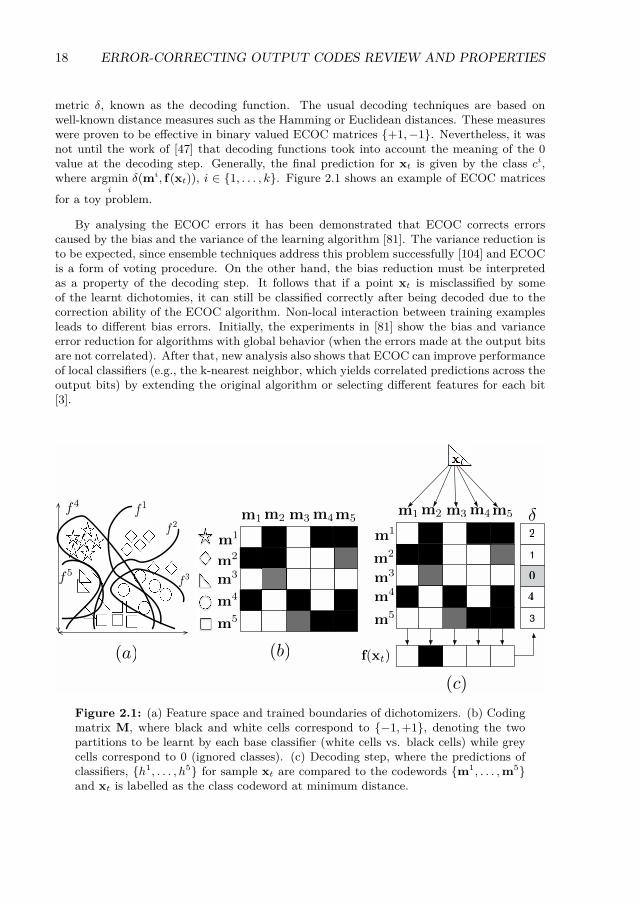
metric δ, known as the decoding function. The usual decoding techniques are based onwell-known distance measures such as the Hamming or Euclidean distances. These measureswere proven to be effective in binary valued ECOC matrices +1,−1. Nevertheless, it wasnot until the work of [47] that decoding functions took into account the meaning of the 0value at the decoding step. Generally, the final prediction for xt is given by the class ci,where argmin

i

δ(mi, f(xt)), i ∈ 1, . . . , k. Figure 2.1 shows an example of ECOC matrices

for a toy problem.

By analysing the ECOC errors it has been demonstrated that ECOC corrects errorscaused by the bias and the variance of the learning algorithm [81]. The variance reduction isto be expected, since ensemble techniques address this problem successfully [104] and ECOCis a form of voting procedure. On the other hand, the bias reduction must be interpretedas a property of the decoding step. It follows that if a point xt is misclassified by someof the learnt dichotomies, it can still be classified correctly after being decoded due to thecorrection ability of the ECOC algorithm. Non-local interaction between training examplesleads to different bias errors. Initially, the experiments in [81] show the bias and varianceerror reduction for algorithms with global behavior (when the errors made at the output bitsare not correlated). After that, new analysis also shows that ECOC can improve performanceof local classifiers (e.g., the k-nearest neighbor, which yields correlated predictions across theoutput bits) by extending the original algorithm or selecting different features for each bit[3].

xt

f(xt)

3

44

00

1

22

(a) (b)

(c)

f3

f2

f1f4

f5

m1

m2

m3

m4

m5

m1

m2

m3

m4

m5

m1m2 m3 m4m5m1m2 m3 m4m5 δ

Figure 2.1: (a) Feature space and trained boundaries of dichotomizers. (b) Codingmatrix M, where black and white cells correspond to −1,+1, denoting the twopartitions to be learnt by each base classifier (white cells vs. black cells) while greycells correspond to 0 (ignored classes). (c) Decoding step, where the predictions ofclassifiers, h1, . . . , h5 for sample xt are compared to the codewords m1, . . . ,m5and xt is labelled as the class codeword at minimum distance.

2.2. ECOC Coding 19

2.2 ECOC CodingIn this section we review state-of-the-art coding designs. We divide the coding designs basedon their membership to the binary or ternary ECOC frameworks.

2.2.1 Binary CodingThe standard binary coding designs are the One vs. All design [111] and the Dense Randomdesign [3]. In One vs. All each dichotomy is defined to distinguish one category from therest of the classes. An example is shown in Figure 2.2(a). The Dense Random codinggenerates a very high number of coding matrices M of length l, where the values −1,+1are equiprobable. In [3] the authors suggested to experimentally set l = 10 log k. From theset of Dense Random matrices generated the optimal one should maximize the minimumHamming distance between the codewords of M, taking into account that each column ofM should contain −1,+1. An example of Dense Random coding is show in Figure 2.2(b).Furthermore, recent works have proposed various problem-dependent binary codings. In[141] the authors propose the Spectral Error-Correcting Output Codes [141], in which theECOC coding corresponds to a subset of thresholded eigenvectors of the graph Laplacian ofsimilarity matrix between categories.

2.2.2 Ternary CodingThe standard ternary codings designs are the One vs. One [125] and Sparse Random strate-gies [3]. The One vs. One strategy consider all possible pairs of classes, having a codelength of k(k−1)

2 . An example of the One vs. One coding design for a 4-class problem isshow in Figure 2.2(c). The Sparse Random coding is similar to the Dense Random design,with the exception that it includes the 0 symbol. In this case, symbols −1,+1, 0 can notbe equiprobable. In [3] the authors suggest an experimental length of l = 15 log k for theDense Random design. In Figure 2.2(d) we show an example of the Sparse Random design.In addition, problem-dependent designs have also been the focus of recent works. In [106],the authors propose the Discriminant ECOC coding which is based on the embedding ofdiscriminant tree structures derived from the problem domain. The binary trees are builtby looking for the sub-sets of classes that maximizes the mutual information between thedata and their respective class labels. Finally, the work of Zhao et. al [142] proposes a dualprojected gradient method embedded on a constrained concave-convex procedure to optimizean objective composed of a measure of expected problem separability, codeword correlationand regularization terms.

2.3 ECOC DecodingIn this section, we review the state-of-the-art on decoding designs. The decoding strategies(independently of the rules they are based on) are divided depending if they were designedto deal with the binary or the ternary ECOC frameworks.

2.3.1 Binary DecodingThe binary decoding designs most frequently applied are: Hamming Decoding [100], InverseHamming Decoding [136], and Euclidean Decoding [3].

20 ERROR-CORRECTING OUTPUT CODES REVIEW AND PROPERTIES

m1

m2

m3

m4

m5

m1m2 m3 m4m5

m1

m2

m3

m4

m5

m1m2 m3 m4m5

m1

m2

m3

m4

m5

m1m2 m3 m4m5

(a) (b) (c)

(d)

m1 m3

m1m2

m2

m3

m4

m5

m4 m5 m6 m7 m8 m9 m10 m11m12 m13 m14 m15

Figure 2.2: (a) ECOC One vs. All coding design. (b) Dense Random coding desing.(c) Sparse Random coding. (d) One vs. One ECOC coding design.

• The Hamming Decoding is defined as follows:

δHD(f(xt),mi)) =l∑

j=1

(1− sign(h(xt)j ·mij))/2 (2.1)

This decoding strategy is based on the error-correcting principles under the assumptionthat the learning task can be modeled as a communication problem, in which classinformation is transmitted over a channel, and two possible symbols can be found ateach position of the sequence [39].

• The Inverse Hamming Decoding introduced in [136] is defined as follows: let Hbe the matrix composed by the Hamming distance measures between the codewordsof M. Each position of H is defined by hij = δHD(mi,mj)∀i, j ∈ 1, . . . , k. H canbe inverted to find the vector containing the k individual class likelihood functions bymeans of:

δIHD(f(xt),mi) = max(H−1r>), (2.2)

where the values of H−1R> can be seen as the proportionality of each class codewordin the test codeword, and r is the vector of Hamming Decoding values of the testcodeword f(xt) for each of the base codewords mi. The practical behavior of the IHDshowed to be very close to the behavior of the HD strategy [47].

2.4. Good practices in ECOC 21

• The Euclidean Decoding is another well-known decoding strategy based the Eu-clidean distance. This measure is defined as follows:

δED(f(xt),mi) =

√√√√ l∑j=1

(h(xt)j −mij)2 (2.3)

2.3.2 Ternary DecodingConcerning the ternary decoding, the state-of-the-art strategies are: Loss-based Decoding[47] and Probabilistic Decoding [47].

• The Loss-based Decoding strategy [47] chooses the label yi that is most consistentwith the predictions h (where h is a real-valued function h : X → y), in the sensethat, if the data sample xt was labeled yt, the total loss on example (xt, yt) would beminimized over choices of yt ∈ 1, . . . , k. Formally, given a Loss-function model, thedecoding measure is the total loss on a proposed data sample (xt, yt):

LB(xt,mi) =l∑

j=1

L(mijh(xt)j), (2.4)

where mijh(xt)j corresponds to the margin and L is a Loss-function that dependson the nature of the binary classifier. The two most common Loss-functions areL(θ) = −θ (Linear Loss-based Decoding (LLB)) and L(θ) = e−θ (Exponential Loss-based Decoding (ELB)). The final decision is achieved by assigning a label to exampleξt according to the class i which codeword mi obtains the minimum score.

• The Probabilistic Decoding strategy proposed in [102] is based on the continuousoutput of the classifier to deal with the ternary decoding. The decoding measure isgiven by:

δPD(mi, F ) = − log

∏j∈1,...,lmij 6=0

P (h(xt)j = mij |hj) +K

, (2.5)

where K is a constant factor that collects the probability mass dispersed on the invalidcodes, and the probability P (h(xt)j = mij |hj) is estimated by means of:

P (h(xt)j = mij |hj) = 11 = emij (υjhj +ωj ) , (2.6)

where vectors υ and ω are obtained by solving an optimization problem [102].

2.4 Good practices in ECOCOnce the coding and decoding designs have been reviewed we analyze which are Goodpractices towards using the ECOC framework. Assume a k-class problem to be learned, thenthe ECOC framework will construct a matrix M ∈ −1, 0,+1k×l in which k codewords willbe chosen from the 3l codes available. Following Newton’s binomial this is be expressed as(3l

k

)which denotes the huge size of the search space. A natural question that researchers

have formulated is: What is a Good ECOC coding matrix? This question has been addressed

22 ERROR-CORRECTING OUTPUT CODES REVIEW AND PROPERTIES

in several works [4, 7, 39, 84, 141], each of them proposing different ways of evaluating anECOC coding matrix, which are summed up in the following three properties:

1. Correction capability: the correction capability is expressed min(δ(mi,mj ))−12 , ∀i, j ∈

1, . . . , k, i 6= j 1. In this sense, if min δ(mi,mj) = 3, ECOC will be able to recoverthe correct multi-class prediction even if b 3−1

2 c = 1 binary classifier misses its predic-tion.

2. Uncorrelated binary sub-problems: the induced binary problems (columns of M)should be as uncorrelated as possible for M to recover binary classifier errors.

3. Use of powerful binary classifiers: since the final class prediction consists of theaggregation of bit predictors, high-capacity binary classifiers are also required to obtainaccurate multi-class predictions.

4. Complexity of dichotomies: easy binary problems will lead to increase overallperformance of the ECOC coding [60, 142].

While exploiting these properties has lead to improvement either in overall model com-plexity [12, 60], scalability [142] or performance [51], we still lack an understanding abouthow the error-correction is distributed between different codewords and how that impactsthe performance of the ECOC performance. This thesis aims to find answer to these issues.

2.5 ECOC constraintsTo better understand ECOC correction we first start by analyzing the constraints of anECOC coding matrix. Given the underlaying intuition of ECOCs in which an codeword mi

is assigned to each class, it follows that not all binary or ternary matrix M ∈ −1,+1, 0 arevalid ECOC coding matrices. Hence, ECOC coding matrices have a certain structure andconstraints that need to be taken into account. These constraints concern the repetitionsof rows in M. Since a repetition of rows will define two different categories with the samecodeword, it implies that an ambiguous coding matrix M will be constructed. Moreover,error-correcting principles of communication theory are based on the assumption that errorsintroduced by each dichotomizer are uncorrelated [39]. In this sense, similar dichotomieswill output correlated outputs, and thus, this situation has to be avoided. In the limit case,equivalent dichotomies will have equivalent outputs, and thus, no correction capability willbe generated. In this sense, when designing ECOC coding matrices these constraints mustbe taken into account. We define a valid ECOC coding matrix M ∈ −1,+1, 0k×l to beconstrained by:

min(δAHD(mi,mk)) ≥ 1, ∀i, j : i 6= j, i, j ∈ [1, . . . , k], (2.7)

min(δHD(mi,mj)) ≥ 1, ∀i, j : i 6= j, i, j ∈ [1, . . . , k], (2.8)

min(δHD(mi,−mj)) ≥ 1, ∀i, j : i 6= j, i, j ∈ [1, . . . , k], (2.9)where δAHD and δHD are the Attenuated Hamming Distance (AHD) [47] and the Ham-

ming Distance (HD), respectively, defined as follows:

δAHD(mi,mj) =n∑k=1

|mki||mkj |I(mki,mkj), (2.10)

1In the case of ternary codes this correction capability can be easily adapted.

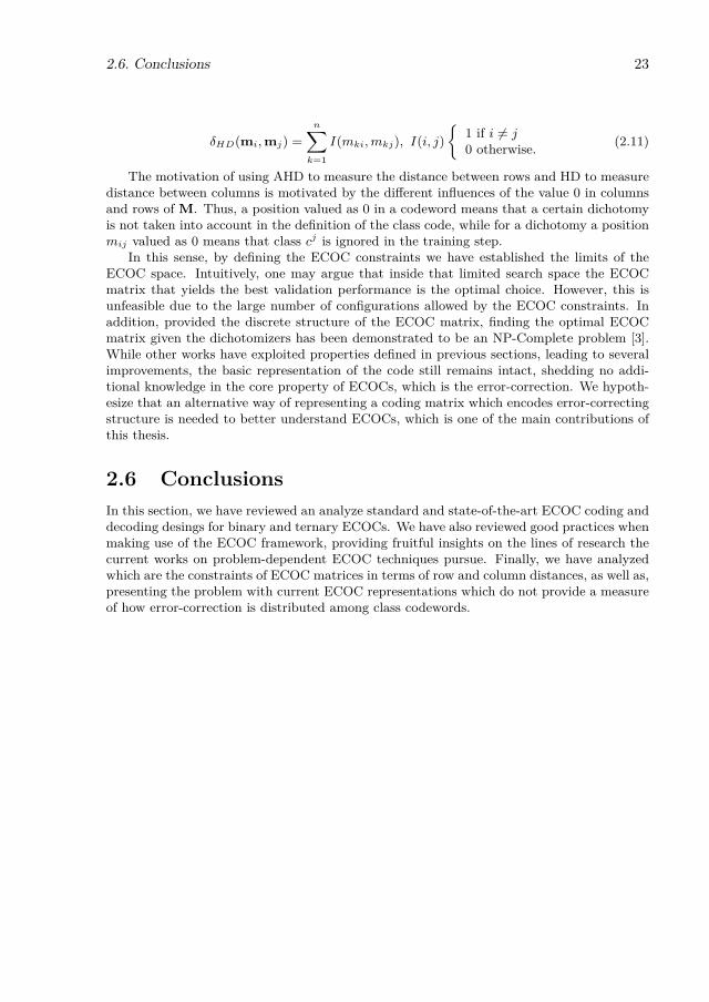
2.6. Conclusions 23

δHD(mi,mj) =n∑k=1

I(mki,mkj), I(i, j)

1 if i 6= j0 otherwise. (2.11)

The motivation of using AHD to measure the distance between rows and HD to measuredistance between columns is motivated by the different influences of the value 0 in columnsand rows of M. Thus, a position valued as 0 in a codeword means that a certain dichotomyis not taken into account in the definition of the class code, while for a dichotomy a positionmij valued as 0 means that class cj is ignored in the training step.

In this sense, by defining the ECOC constraints we have established the limits of theECOC space. Intuitively, one may argue that inside that limited search space the ECOCmatrix that yields the best validation performance is the optimal choice. However, this isunfeasible due to the large number of configurations allowed by the ECOC constraints. Inaddition, provided the discrete structure of the ECOC matrix, finding the optimal ECOCmatrix given the dichotomizers has been demonstrated to be an NP-Complete problem [3].While other works have exploited properties defined in previous sections, leading to severalimprovements, the basic representation of the code still remains intact, shedding no addi-tional knowledge in the core property of ECOCs, which is the error-correction. We hypoth-esize that an alternative way of representing a coding matrix which encodes error-correctingstructure is needed to better understand ECOCs, which is one of the main contributions ofthis thesis.

2.6 ConclusionsIn this section, we have reviewed an analyze standard and state-of-the-art ECOC coding anddecoding desings for binary and ternary ECOCs. We have also reviewed good practices whenmaking use of the ECOC framework, providing fruitful insights on the lines of research thecurrent works on problem-dependent ECOC techniques pursue. Finally, we have analyzedwhich are the constraints of ECOC matrices in terms of row and column distances, as well as,presenting the problem with current ECOC representations which do not provide a measureof how error-correction is distributed among class codewords.

24 ERROR-CORRECTING OUTPUT CODES REVIEW AND PROPERTIES

Chapter 3

In this chapter we introduce the Separability matrix as a way to represent the error-correctingstructure of an ECOC coding matrix. Although the concept of error-correction has alwaysbeen in the core of all ECOC studies, up to this moment there has not been the need ofdefining explicitly a matrix of this kind. This is mainly due to the fact that predefinedor random strategies assume that the coding matrix should have equidistant codewords orat least be as close as possible to an equidistant distribution [3]. The Separability matrixexplicitly encodes the pairwise separation-distance between all pairs of codewords in M.

3.1 The Separability matrixOne of the main properties of a good ECOC coding matrix is the correcting capability (thenumber of errors in binary classifiers that ECOC is able to correct). In literature, the correc-tion capability of a coding matrix M is defined as min(δ(mi,mj ))−1

2 , ∀i, j ∈ 1, . . . , k, i 6= j.Therefore, distance between codewords and correction capability are directly related. Giventhis close relationship between distance and correction capability, we define the Separabilitymatrix H, as follows:

Given an ECOC coding matrix M ∈ −1, 0,+1k×l, the Separability matrix H ∈ Rk×kcontains the distances between all pairs of codes in M. Let mi,mj be two codewords,the Separability matrix H at position (i, j), defined as hij , contains the Attenuated Ham-ming Distance between the codewords mi,mj, defined as δAHD(mi,mj). An example ofSeparability matrices for different coding designs is shown in Figure 3.1.

If we analyze the Separability matrix H of predefined ECOC coding designs [111, 125], wefind that H is constant in all off-diagonal values. This means that codewords are equidistant,as shown in Figure 3.1(e)(h). In fact, when dealing with predefined codings, the Separabilitymatrix makes little sense and has been overlooked since all off-diagonal values are constant.Nevertheless, in problem-dependent coding strategies the Separability matrix acquires agreat value, since it shows which codewords are prone to have more errors due to the lackof error-correction capability.

3.2 From global to pair-wise correction capabilityCorrection capability has been a core objective of problem-dependent designs of M. Inprevious works, different authors have always agreed on defining correction capability for anECOC coding matrix as a scalar value [3, 39, 60, 62, 84, 141]. Hence, min(H) is expectedto be large in order for M to recover from as many binary classifier errors as possible.

25

26A NOVEL REPRESENTATION FOR ECOCS: THE SEPARABILITY MATRIX

However, since H expresses the Attenuated Hamming distance between rows of M, onecan alternatively express the correction capability in a pair-wise fashion, allowing for adeeper understanding of how correction is distributed among codewords. Figure 3.2 shows anexample of global and pair-wise correction capabilities calculation. Recall that the⊕ operatorbetween two vectors denotes its concatenation. Thus, we define the pair-wise correctioncapability as follows:

• The pair-wise correction capability of codewords mi and mj is expressed as:bmin(hi⊕hj )−1

2 c, where we only consider off-diagonal values of H. This means thata sample of class ci is correctly discriminated from class cj even if bmin(hi⊕hj ))−1

2 cbinary classifiers miss their predictions.

Note that though in Figure 3.2 the global correction capability of M is 0, there arepairs of codewords with a higher correction, e.g. m2 and m8. In this case the globalcorrection capability as defined in literature is overlooking ECOC coding characteristicsthat can potentially be exploited. This novel way of expressing the correction capability ofan ECOC matrix enables a better understanding of how ECOC coding matrices distributetheir correction capability, and gives an insight on how to design coding matrices.

3.3 ConclusionsIn this chapter we have show that the standard way of analyzing the error-correction of anECOC clearly overlooks crucial aspect in the pair-wise relationships between codewords thatcan be beneficial to exploit. We have also shown how to compute the Separability Matrix Hgiven a ECOC coding matrix M and what structure is expected for state-of-the-art codingdesigns. However, we still need to solve various issues to exploit this representation:

• How to estimate a suitable Separability matrix for a multi-class problem given onlythe multi-class data xi, yi : i ∈ 1, . . . , n, which we denote as the Design MatrixD ∈ Rk×k. This problem intuitively tackles how error-correction should be allocated.The open question is of the following form: Should correction be allocated accordingto those classes that are more prone to error, in order for them to have better recoverybehavior (i.e. following a "no class is left behind" criteria)? Or should correction beallocated to easily separable classes [60, 141, 142] (i.e. following a "hard classes areleft behind" scheme)?

• Given the Design Matrix D how to obtain the ECOC matrix M.

Both of this issues are analyzed in Section 5.1.

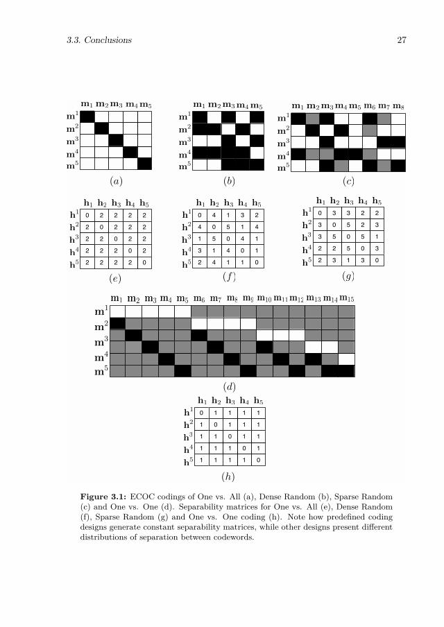
3.3. Conclusions 27

m1 m3

m1

m2

m2

m3

m4

m5

m1 m3

m1

m2

m2

m3

m4

m5

m1 m3

m1m2

m2

m3

m4

m5

m1 m3

m1

m2

m2

m3

m4

m5

m4 m5 m6 m7 m8 m9 m10

m4m5m4m5 m4m5 m6 m7 m8

2

2

2

0

2

0

2

2

2

2

2

2

2

0

2

2

2

2

2

0

0

2

2

2

2

h1 h2 h3 h4 h5

h1

h2

h3

h4

h5

1

1

2

0

4

0

3

4

1

1

4

4

1

0

1

2

1

3

4

0

0

1

5

5

4

h1 h2 h3 h4 h5

h1

h2

h3

h4

h5

1

1

1

0

1

0

1

1

1

1

1

1

1

0

1

1

1

1

1

0

0

1

1

1

1

h1 h2 h3 h4 h5

h1

h2

h3

h4

h5

3

1

2

0

3

0

2

5

3

2

5

3

3

0

2

2

3

2

3

0

0

1

5

5

3

h1 h2 h3 h4 h5

h1

h2

h3

h4

h5

m11m12 m13 m14 m15

(a) (b) (c)

(d)

(e) (f) (g)

(h)

Figure 3.1: ECOC codings of One vs. All (a), Dense Random (b), Sparse Random(c) and One vs. One (d). Separability matrices for One vs. All (e), Dense Random(f), Sparse Random (g) and One vs. One coding (h). Note how predefined codingdesigns generate constant separability matrices, while other designs present differentdistributions of separation between codewords.

28A NOVEL REPRESENTATION FOR ECOCS: THE SEPARABILITY MATRIX

!

"

#

$

$

!

#

!

%

"

%

!

#

$

$

&

!

#

$

$

&

$

$

#

%

#

&

!

!

&

%

!

!

#

$

$

#

&

$

$

" !#

&

$

!

!

#

#

& %

!

!

"

%

! &

$

$

# %

$

%

!

X H

h2

h8

x2

x8

⌊min(H)− 1

2⌋ = 0 ⌊min(h2 ⊕ h8)− 1

2⌋ = 1

M

m2

m8

Figure 3.2: Example of global versus pair-wise correction capability. On the left sideof the figure the calculation of the global correction capability is shown. The rightside of the image shows a sample of pair-wise correction calculation for codewordsm2 and m8.

Part II

Learning ECOCrepresentations

29

Chapter 4

Learning ECOCs using GeneticAlgorithms

Due to the nature of the Error-Correcting Output Codes space [62, 89, 90] Genetic Algo-rithms (GA) have been applied in this scenario to learn problem-dependent ECOC codingmatrices. In particular, the ECOC search space has been proven to be non-continuous andnon-differentiable, thus making the use of Genetic Algorithms a popular choice . In thischapter we present our contributions to state-of-the-art Genetic Algorithms for ECOCs, de-veloping methods based both on standard and non standard GAs that are compliant withthe Error-Correcting Output Codes constraints.

4.1 Towards Reducing the ECOC Code LengthThe coding step of the ECOC framework has been widely studied in literature, obtainingeither predefined [111, 125], random [3] or problem-dependent [49, 105, 106, 122, 145] codingdesigns. The most well-known coding schemes are the predefined ones, such as, One vs.One [125] and One vs. All [111] designs, in which

(k2

)and k dichotomies are defined,

respectively. In the One vs. One scheme all the possible pair-wise groups of the k categoriesare defined, while in the One vs. All scheme each dichotomy is responsible of discriminatingone class against the rest of the classes. In contra-position, some works in literature havestated that random designs [4], with code length of 10, 15 · log2(k) can perform as well aspredefined codes. However, predefined or random designs do not exploit the problem-domaininformation.

In this sense, some works in literature have proposed the use of problem-dependent ECOCcoding matrices. Problem-dependent coding designs lay on the assumption that predefinedand random codes may not be suitable to solve a given problem since they do not take intoaccount the underlying distribution of the classes in the multi-class problem. In [106] theauthors proposed the DECOC coding design of length k − 1 in which a tree structure isembedded in the ECOC coding matrix, where nodes correspond to classes that maximize asplit criterion. In the trend of the previous works, [49] proposed the same tree embeddingwhere the nodes correspond to the most difficult meta-classes to be learnt. Other works aimto treat the problem either by soft weight sharing methods [5] or by using EM algorithm tofind the optimal decomposition of the multi-class problem [128]. However, in [111] Rifkin et.al stated that when using high capacity dichotomizers the code length can be reduced with

31

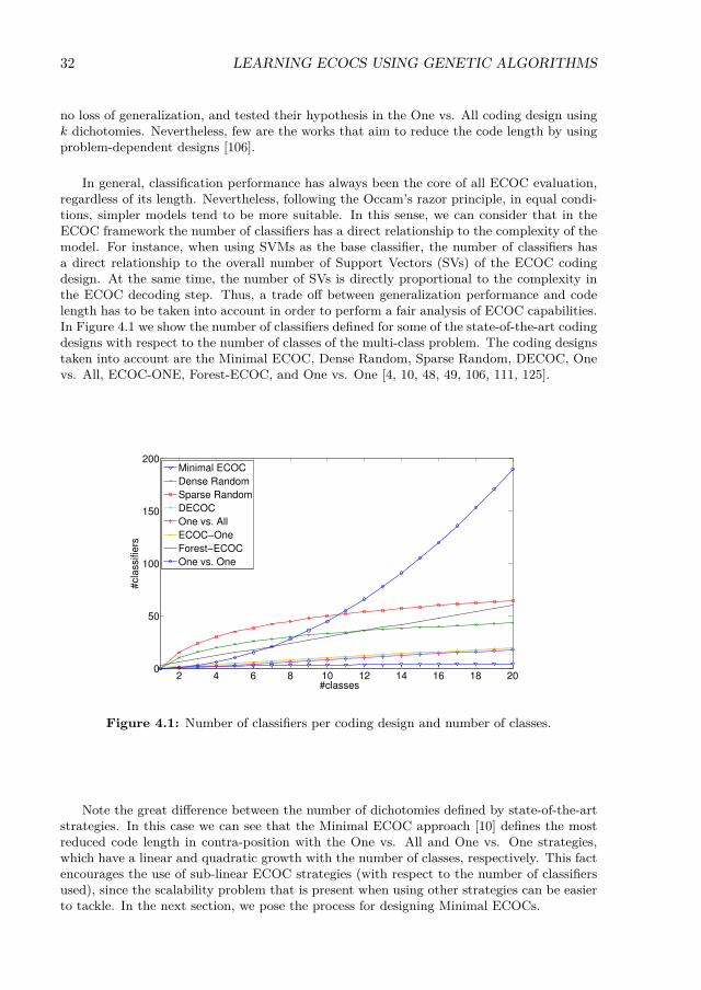
32 LEARNING ECOCS USING GENETIC ALGORITHMS

no loss of generalization, and tested their hypothesis in the One vs. All coding design usingk dichotomies. Nevertheless, few are the works that aim to reduce the code length by usingproblem-dependent designs [106].

In general, classification performance has always been the core of all ECOC evaluation,regardless of its length. Nevertheless, following the Occam’s razor principle, in equal condi-tions, simpler models tend to be more suitable. In this sense, we can consider that in theECOC framework the number of classifiers has a direct relationship to the complexity of themodel. For instance, when using SVMs as the base classifier, the number of classifiers hasa direct relationship to the overall number of Support Vectors (SVs) of the ECOC codingdesign. At the same time, the number of SVs is directly proportional to the complexity inthe ECOC decoding step. Thus, a trade off between generalization performance and codelength has to be taken into account in order to perform a fair analysis of ECOC capabilities.In Figure 4.1 we show the number of classifiers defined for some of the state-of-the-art codingdesigns with respect to the number of classes of the multi-class problem. The coding designstaken into account are the Minimal ECOC, Dense Random, Sparse Random, DECOC, Onevs. All, ECOC-ONE, Forest-ECOC, and One vs. One [4, 10, 48, 49, 106, 111, 125].

2 4 6 8 10 12 14 16 18 200

50

100

150

200

#classes

#cla

ssifie

rs

Minimal ECOC

Dense Random

Sparse Random

DECOC

One vs. All

ECOC−One

Forest−ECOC

One vs. One

Figure 4.1: Number of classifiers per coding design and number of classes.

Note the great difference between the number of dichotomies defined by state-of-the-artstrategies. In this case we can see that the Minimal ECOC approach [10] defines the mostreduced code length in contra-position with the One vs. All and One vs. One strategies,which have a linear and quadratic growth with the number of classes, respectively. This factencourages the use of sub-linear ECOC strategies (with respect to the number of classifiersused), since the scalability problem that is present when using other strategies can be easierto tackle. In the next section, we pose the process for designing Minimal ECOCs.

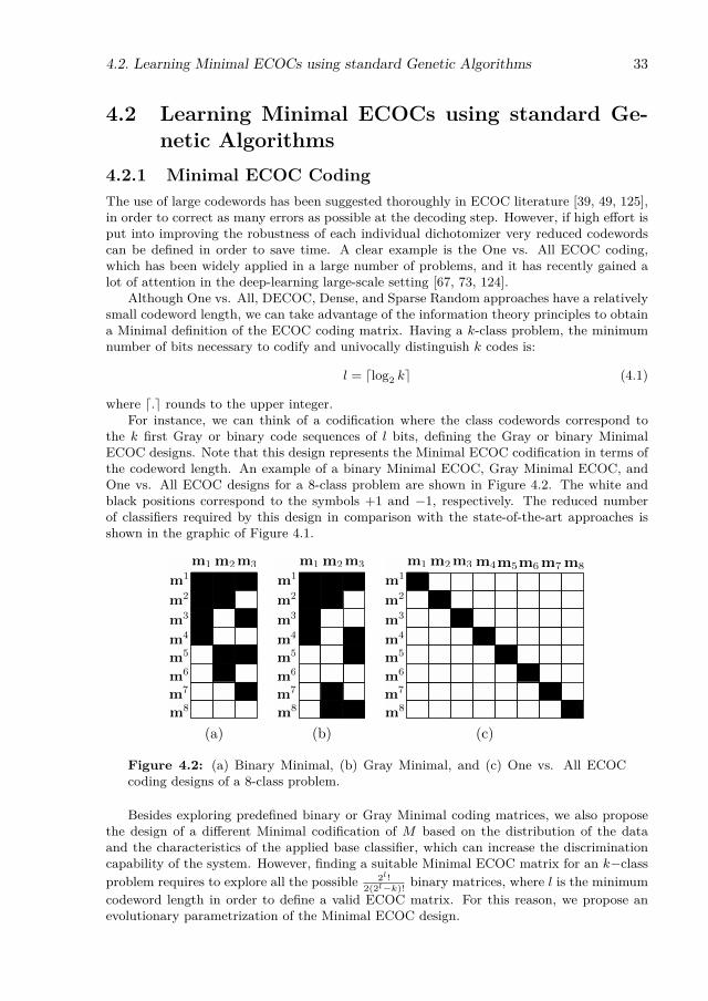
4.2. Learning Minimal ECOCs using standard Genetic Algorithms 33

4.2 Learning Minimal ECOCs using standard Ge-netic Algorithms

4.2.1 Minimal ECOC CodingThe use of large codewords has been suggested thoroughly in ECOC literature [39, 49, 125],in order to correct as many errors as possible at the decoding step. However, if high effort isput into improving the robustness of each individual dichotomizer very reduced codewordscan be defined in order to save time. A clear example is the One vs. All ECOC coding,which has been widely applied in a large number of problems, and it has recently gained alot of attention in the deep-learning large-scale setting [67, 73, 124].

Although One vs. All, DECOC, Dense, and Sparse Random approaches have a relativelysmall codeword length, we can take advantage of the information theory principles to obtaina Minimal definition of the ECOC coding matrix. Having a k-class problem, the minimumnumber of bits necessary to codify and univocally distinguish k codes is:

l = dlog2 ke (4.1)

where d.e rounds to the upper integer.For instance, we can think of a codification where the class codewords correspond to

the k first Gray or binary code sequences of l bits, defining the Gray or binary MinimalECOC designs. Note that this design represents the Minimal ECOC codification in terms ofthe codeword length. An example of a binary Minimal ECOC, Gray Minimal ECOC, andOne vs. All ECOC designs for a 8-class problem are shown in Figure 4.2. The white andblack positions correspond to the symbols +1 and −1, respectively. The reduced numberof classifiers required by this design in comparison with the state-of-the-art approaches isshown in the graphic of Figure 4.1.

m1 m3

m1

m8

m2

m2

m3

m4

m5

m6

m7

m1 m3

m1

m8

m2

m2

m3

m4

m5

m6

m7

m1 m3

m1

m8

m2

m2

m3

m4

m5

m6

m7

m4m5m6m7 m8

(a) (b) (c)

Figure 4.2: (a) Binary Minimal, (b) Gray Minimal, and (c) One vs. All ECOCcoding designs of a 8-class problem.

Besides exploring predefined binary or Gray Minimal coding matrices, we also proposethe design of a different Minimal codification of M based on the distribution of the dataand the characteristics of the applied base classifier, which can increase the discriminationcapability of the system. However, finding a suitable Minimal ECOC matrix for an k−classproblem requires to explore all the possible 2l!

2(2l−k)! binary matrices, where l is the minimumcodeword length in order to define a valid ECOC matrix. For this reason, we propose anevolutionary parametrization of the Minimal ECOC design.

34 LEARNING ECOCS USING GENETIC ALGORITHMS

4.2.2 Evolutionary Minimal ECOC LearningWhen defining a Minimal design of an ECOC, the possible loss of generalization performancedue the reduced number of dichotomies has to be taken into account. In order to deal withthis problem an evolutionary optimization process is used to find a Minimal ECOC withhigh generalization capability.

In order to show the parametrization complexity of the Minimal ECOC design, we firstprovide an estimation of the number of different possible ECOC matrices that we can build,and therefore, the search space cardinality. We approximate this number using some simplecombinatorial principles. First of all, if we have an k−class problem and l possible bitsto represent all the classes, we have a set with 2l different codewords. In order to buildan ECOC matrix, we select k codewords from the set without reposition. In other words,taking k codewords from a variation of 2l. In combinatorics this number is represented as(k2l

), which means that we can construct 2l!

(2l−k)! different ECOC matrices. Nevertheless, inthe ECOC framework, one matrix and its opposite (swapping all minus ones by ones andvice-versa) are considered as the same matrix, since both represent the same partitions of thedata. Therefore, the approximated number of possible ECOC matrices with the minimumnumber of classifiers is 2l!

2(2l−k)! . In addition to the huge cardinality, it is easy to show that thisspace is non continuous neither differentiable, because a change in just one bit of the matrixmay produce a wrong coding design (i.e one in which two rows of M are equivalent). In [34]the authors proved that finding the optimal codeword of the matrix M is computationallyunfeasible since it is an NP-complete problem.

In this type of scenarios evolutionary approaches are often introduced with good results.Evolutionary algorithms are a wide family of methods that are inspired on Darwin’s evo-lution theory, and are formulated as optimization processes where the solution space is notdifferentiable or is not well defined, hence this kind of approaches can only guarantee to findsuboptimal solutions in the best case.

In these cases, the simulation of natural evolution processes using computers results instochastic optimization techniques which often outperform classical methods of optimizationwhen applied to difficult real-world problems. Although the most used and studied evolu-tionary algorithms are the Genetic Algorithms, the Population Based Incremental Learning(PBIL) by Baluja and Caruana [9] proposed a new family of evolutionary methods whichis striving to find a place in this field. In contrast to GAs, this new algorithms considereach value in the chromosome as a random variable, and their goal is to learn a probabilitymodel to describe the characteristics of good individuals. In the case of PBIL, if a binarychromosome is used, a uniform distribution is learnt in order to estimate the probability ofeach variable to be one or zero. In this thesis we report experiments made with both GAand PBIL evolutionary strategies.

Problem encoding

The first step in order to use an evolutionary algorithm is to define the problem encoding,which consists of the representation of a certain solution or point in the search space by meansof a genotype or alternatively a chromosome [70]. When the solutions or individuals aretransformed in order to be represented in a chromosome, the original values (the individuals)are referred as phenotypes, and each one of the possible settings for a phenotype is the allele.Binary encoding is the most common, mainly because first works about GA used this type ofencoding. In binary encoding, every chromosome is a string of bits. Although this encodingis often not natural for many problems and sometimes corrections must be performed aftercrossover and/or mutation, in our case, the chromosomes represent binary ECOC matrices,

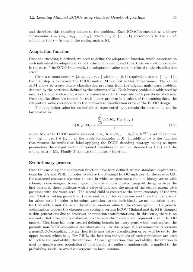
4.2. Learning Minimal ECOCs using standard Genetic Algorithms 35

and therefore, this encoding adapts to the problem. Each ECOC is encoded as a binarychromosome s = m11,m12, . . . ,mkl, where mij ∈ −1,+1 corresponds to the i − thcolumn of the j − th row in the coding matrix M.

Adaptation function

Once the encoding is defined, we need to define the adaptation function, which associates toeach individual its adaptation value to the environment, and thus, their survival probability.In the case of the ECOC framework, the adaptation value must be related to the classificationerror.

Given a chromosome s = s0, s1, . . . , sk×l with si ∈ 0, 1 (equivalent to si ∈ −1,+1),the first step is to recover the ECOC matrix M codified in this chromosome. The valuesof M allows to create binary classification problems from the original multi-class problem,denoted by the partitions defined by the columns ofM . Each binary problem is addressed bymeans of a binary classifier, which is trained in order to separate both partitions of classes.Once the classifiers are trained for each binary problem in a subset of the training data, theadaptation value corresponds to the multi-class classification error of the ECOC design.

The adaptation value for an individual represented by a certain chromosome si can beformulated as:

E(X,y,Mi) =

j′∑j=1I(δ(Mi, f(xj)), yj)

j′(4.2)

where Mi is the ECOC matrix encoded in si, X = x1, . . . ,xtr ∈ R1×f a set of samples,y = y1, . . . , ytr ∈ [1, . . . , k] the labels for samples in X. In addition, δ is the functionthat returns the multi-class label applying the ECOC decoding strategy, taking as inputparameters the output vector of trained classifiers on sample, denoted as f(xj) and thecoding matrix Mi. Finally I denotes the indicator function.

Evolutionary process

Once the encoding and adaptation function have been defined, we use standard implementa-tions for GA and PBIL, in order to evolve the Minimal ECOC matrices. In the case of GA,the scattered crossover operator is used, in which we generate a random binary vector witha binary value assigned to each gene. The first child is created using all the genes from thefirst parent in those positions with a value of one, and the genes of the second parent withpositions with the value zero. The second child is created as the complementary of the firstone. That is, taking genes from the second parent for values one and from the first parentfor values zero. In order to introduce variations to the individuals, we use mutation opera-tor that adds a unit Gaussian distributed random value to the chosen gene. In the geneticoptimization process the chromosome coding a certain ECOC Minimal matrix M is changedwithin generations due to crossover or mutation transformations. In this sense, there is nowarranty that after any transformations the new chromosome will represent a valid ECOCmatrix. This issue has been treated defining bounds for every gene, which contemplate thepossible non-ECOC-compliant transformations. In this scope, if a chromosome representsa non-ECOC-compliant matrix then its fitness value (classification error) will be set to theupper bound, which is 1. For PBIL, the best two individuals of each population are usedto update the probability distribution. At each generation, this probability distribution isused to sample a new population of individuals. An uniform random noise is applied to theprobability model to avoid convergence to local minima.

36 LEARNING ECOCS USING GENETIC ALGORITHMS

Finally, in both evolutionary strategies we adopt an Island Model evolution scheme inorder to exploit a more coarse grain parallel model. The main idea is to split a population ofindividuals into sub-populations. If each sub-population is evolved independently from theothers, genetic drift will tend to drive these populations in different directions. By introduc-ing migration, the Island Model is able to exploit differences in the various sub-populations(this variation in fact represents a source of genetic diversity). Each sub-population is anisland and there is a chance movement of genetic material from one island to another.

Training the binary classifiers

In [111], Rifkin concludes that the number of classifiers in the ECOC problem can be success-fully reduced using high capacity classifiers. In this scope, in [72] SVMs with a RBF kernelhave demonstrated to have V C − dimension = ∞. Therefore, in this paper we adopt theSupport Vector Machines with Gaussian Radial Basis Functions kernel (SVM-RBF) as ourbase classifier. Training a SVM implies the selection of a subset of data points (the supportvectors), which are used in order to build the classification boundaries. In the specific case ofSVMs with Gaussian RBF kernels, we need to optimize the kernel parameter γ = 1

σ2 and theregularizer C, which have a close relation to the data distribution. While the support vectorsselection is part of the SVM learning algorithm, and therefore, is clearly defined, finding thebest C and γ is addressed in literature with various heuristic or brute-force approaches. Themost common approach is the use of cross-validation processes which select the best pair ofparameters for a discretization of the parameters space. Nevertheless, this can be viewed asanother optimization problem and it can be faced using evolutionary algorithms. For eachbinary problem, defined by one column of the ECOC matrix, we use Genetic Algorithms inorder to find good values for C and γ, using the same settings than in [90], where individualscorrespond to a pairs of genes, and each gene corresponds to the binary codification of afloating point value. As for any model selection procedure, this parameter estimation isperformed under a 2-fold cross-validation measurement to reduce the overfitting bias. Moredetails can be found in [80].

Figure 4.3 illustrates an iteration of the evolutionary Minimal ECOC parametrizationfor a toy problem of three categories. Given an input chromosome s1 that codifies a validMinimal matrix M, for each dichotomizer, an evolutionary approximation of the classifierparameters C, γ is performed. From left to right of the image, we show the Minimal ECOCmatrix codifying the 3-class problem, the feature spaces, and the search space of C, γ.Each decision boundary shows a possible certain solution given by the GA. In this sense, theGA starts giving solutions (pairs C, γ) that do not fit a robust decision boundary at thebeginning, but after convergence, the GA increases the adjustment of these boundaries. Thefinal parameters are those that minimize the error over a validation subset. The evolution ofthe best individual is shown in the toy error surface on the right of the image. Finally, theevolution of this matrix returns the adaptation value E of the current individual (currentMinimal configuration), estimated as the minimum classification error computed.

This coding optimization process is computationally more expensive than the standardapproaches since for every Minimal coding matrix M all the binary classifiers h1 . . . hl haveto be optimized. Nevertheless, large-scale multi-classification problems which are typicallycomputationally unfeasible using standard coding designs can be treated with this approach,since this optimization is only applied for a reduced number of dichotomizers. Furthermore,we use as speed up hack by storing a cache of trained classifiers. Consider a random it-eration of the optimization. In this iteration, every Minimal coding matrix will define aset of bi-partitions m1, . . . ,ml to be learnt by a set of dichotomizers h1 . . . hl. In fact,we can assume that a certain bi-partition mi learnt by a certain dichotomizer hi will be

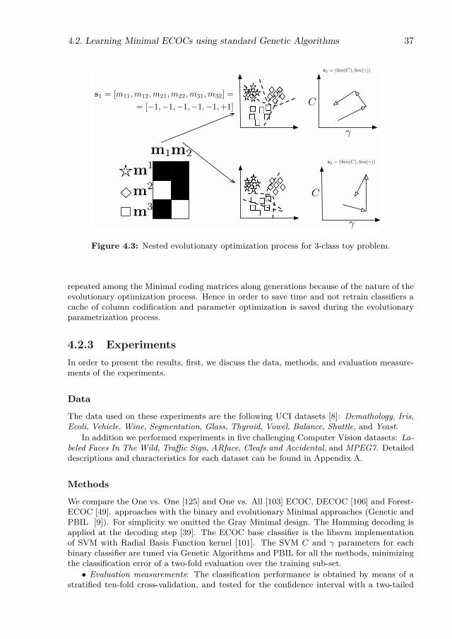
4.2. Learning Minimal ECOCs using standard Genetic Algorithms 37

m1

m1

m2

m2

m3

C

γ

C

γ

s1 = [m11,m12,m21,m22,m31,m32] =

= [−1,−1,−1,−1,−1,+1]

s2 = (bin(C), bin(γ))

s2 = (bin(C), bin(γ))

Figure 4.3: Nested evolutionary optimization process for 3-class toy problem.

repeated among the Minimal coding matrices along generations because of the nature of theevolutionary optimization process. Hence in order to save time and not retrain classifiers acache of column codification and parameter optimization is saved during the evolutionaryparametrization process.

4.2.3 ExperimentsIn order to present the results, first, we discuss the data, methods, and evaluation measure-ments of the experiments.

Data

The data used on these experiments are the following UCI datasets [8]: Demathology, Iris,Ecoli, Vehicle, Wine, Segmentation, Glass, Thyroid, Vowel, Balance, Shuttle, and Yeast.

In addition we performed experiments in five challenging Computer Vision datasets: La-beled Faces In The Wild, Traffic Sign, ARface, Cleafs and Accidental, and MPEG7. Detaileddescriptions and characteristics for each dataset can be found in Appendix A.

Methods

We compare the One vs. One [125] and One vs. All [103] ECOC, DECOC [106] and Forest-ECOC [49]. approaches with the binary and evolutionary Minimal approaches (Genetic andPBIL [9]). For simplicity we omitted the Gray Minimal design. The Hamming decoding isapplied at the decoding step [39]. The ECOC base classifier is the libsvm implementationof SVM with Radial Basis Function kernel [101]. The SVM C and γ parameters for eachbinary classifier are tuned via Genetic Algorithms and PBIL for all the methods, minimizingthe classification error of a two-fold evaluation over the training sub-set.• Evaluation measurements: The classification performance is obtained by means of a

stratified ten-fold cross-validation, and tested for the confidence interval with a two-tailed

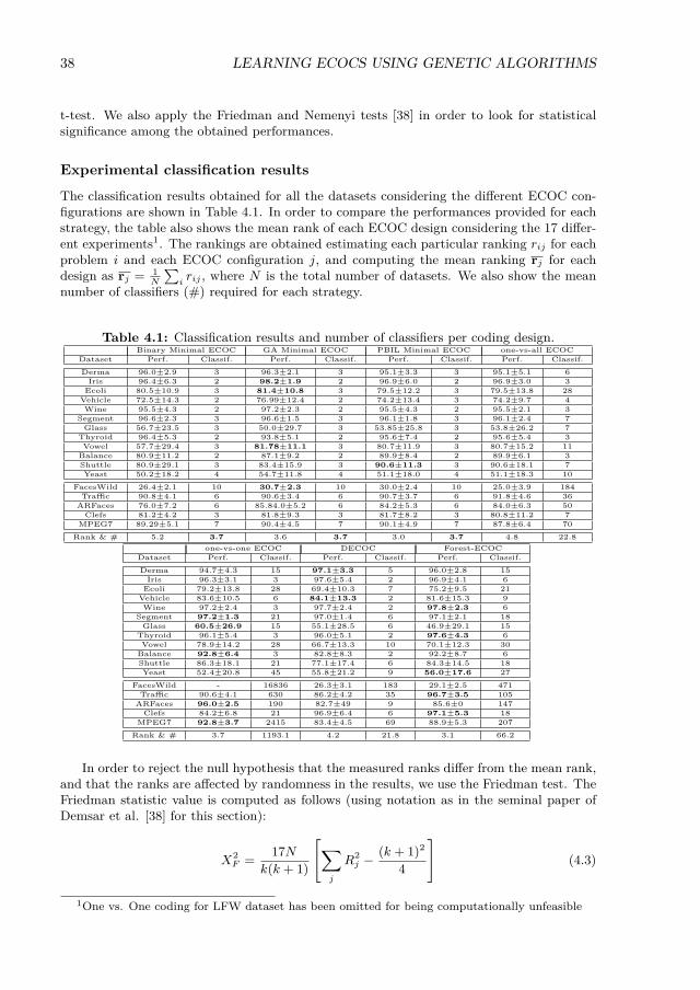
38 LEARNING ECOCS USING GENETIC ALGORITHMS

t-test. We also apply the Friedman and Nemenyi tests [38] in order to look for statisticalsignificance among the obtained performances.

Experimental classification results

The classification results obtained for all the datasets considering the different ECOC con-figurations are shown in Table 4.1. In order to compare the performances provided for eachstrategy, the table also shows the mean rank of each ECOC design considering the 17 differ-ent experiments1. The rankings are obtained estimating each particular ranking rij for eachproblem i and each ECOC configuration j, and computing the mean ranking rj for eachdesign as rj = 1

N

∑irij , where N is the total number of datasets. We also show the mean

number of classifiers (#) required for each strategy.

Table 4.1: Classification results and number of classifiers per coding design.Binary Minimal ECOC GA Minimal ECOC PBIL Minimal ECOC one-vs-all ECOC

Dataset Perf. Classif. Perf. Classif. Perf. Classif. Perf. Classif.

Derma 96.0±2.9 3 96.3±2.1 3 95.1±3.3 3 95.1±5.1 6Iris 96.4±6.3 2 98.2±1.9 2 96.9±6.0 2 96.9±3.0 3Ecoli 80.5±10.9 3 81.4±10.8 3 79.5±12.2 3 79.5±13.8 28Vehicle 72.5±14.3 2 76.99±12.4 2 74.2±13.4 3 74.2±9.7 4Wine 95.5±4.3 2 97.2±2.3 2 95.5±4.3 2 95.5±2.1 3

Segment 96.6±2.3 3 96.6±1.5 3 96.1±1.8 3 96.1±2.4 7Glass 56.7±23.5 3 50.0±29.7 3 53.85±25.8 3 53.8±26.2 7

Thyroid 96.4±5.3 2 93.8±5.1 2 95.6±7.4 2 95.6±5.4 3Vowel 57.7±29.4 3 81.78±11.1 3 80.7±11.9 3 80.7±15.2 11Balance 80.9±11.2 2 87.1±9.2 2 89.9±8.4 2 89.9±6.1 3Shuttle 80.9±29.1 3 83.4±15.9 3 90.6±11.3 3 90.6±18.1 7Yeast 50.2±18.2 4 54.7±11.8 4 51.1±18.0 4 51.1±18.3 10

FacesWild 26.4±2.1 10 30.7±2.3 10 30.0±2.4 10 25.0±3.9 184Traffic 90.8±4.1 6 90.6±3.4 6 90.7±3.7 6 91.8±4.6 36ARFaces 76.0±7.2 6 85.84.0±5.2 6 84.2±5.3 6 84.0±6.3 50Clefs 81.2±4.2 3 81.8±9.3 3 81.7±8.2 3 80.8±11.2 7

MPEG7 89.29±5.1 7 90.4±4.5 7 90.1±4.9 7 87.8±6.4 70

Rank & # 5.2 3.7 3.6 3.7 3.0 3.7 4.8 22.8one-vs-one ECOC DECOC Forest-ECOC

Dataset Perf. Classif. Perf. Classif. Perf. Classif.

Derma 94.7±4.3 15 97.1±3.3 5 96.0±2.8 15Iris 96.3±3.1 3 97.6±5.4 2 96.9±4.1 6Ecoli 79.2±13.8 28 69.4±10.3 7 75.2±9.5 21Vehicle 83.6±10.5 6 84.1±13.3 2 81.6±15.3 9Wine 97.2±2.4 3 97.7±2.4 2 97.8±2.3 6

Segment 97.2±1.3 21 97.0±1.4 6 97.1±2.1 18Glass 60.5±26.9 15 55.1±28.5 6 46.9±29.1 15

Thyroid 96.1±5.4 3 96.0±5.1 2 97.6±4.3 6Vowel 78.9±14.2 28 66.7±13.3 10 70.1±12.3 30Balance 92.8±6.4 3 82.8±8.3 2 92.2±8.7 6Shuttle 86.3±18.1 21 77.1±17.4 6 84.3±14.5 18Yeast 52.4±20.8 45 55.8±21.2 9 56.0±17.6 27

FacesWild - 16836 26.3±3.1 183 29.1±2.5 471Traffic 90.6±4.1 630 86.2±4.2 35 96.7±3.5 105ARFaces 96.0±2.5 190 82.7±49 9 85.6±0 147Clefs 84.2±6.8 21 96.9±6.4 6 97.1±5.3 18

MPEG7 92.8±3.7 2415 83.4±4.5 69 88.9±5.3 207

Rank & # 3.7 1193.1 4.2 21.8 3.1 66.2

In order to reject the null hypothesis that the measured ranks differ from the mean rank,and that the ranks are affected by randomness in the results, we use the Friedman test. TheFriedman statistic value is computed as follows (using notation as in the seminal paper ofDemsar et al. [38] for this section):

X2F = 17N

k(k + 1)

[∑j

R2j −

(k + 1)2

4

](4.3)

1One vs. One coding for LFW dataset has been omitted for being computationally unfeasible

4.2. Learning Minimal ECOCs using standard Genetic Algorithms 39

In our case, with k = 7 methods to compare, X2F = −9.92. Since this value is undesirable

conservative, Iman and Davenport proposed a corrected statistic:

FF = (N − 1)X2F

N(k − 1)−X2F

(4.4)

Applying this correction we obtain FF = 1.72. With seven methods and seventeenexperiments, FF is distributed according to the F distribution with 42 and 272 degrees offreedom. The critical value of F (42, 272) for 0.05 is 1.45. As the value of FF is higher than1.45 we can reject the null hypothesis.

Once we have checked for the non-randomness of the results, we can perform an aposthoc test to check if one of the techniques can be singled out. For this pourpose we use theNemenyi test. The Nemenyi statistic is obtained as follows:

CD = qα

√k(k + 1)

6N (4.5)

In our case with k = 7 methods to compare and N = 17 experiments the critical valuefor a 90% of confidence is CD = 1.33 ·

√42102 = 0.9855. This result shows that there

exists a statically significant difference between using two groups of methods. The groupof the top performers include the Evolutionary Minimal, Forest-ECOC and One vs. Onecodings, versus the group of the worst performers which includes the Binary Minimal, Onevs. All and DECOC codings. These results are very promising since following the Occamrazor’s principles in equal conditions simpler models tend to be more useful. In addition,analyzing the mean rank we find that Evolutionary Minimal approaches are the two firstin rank followed by Forest-ECOC and One vs. One coding. This result is very satisfactoryand encourages the use of the Minimal approach since similar (or even better) results canbe obtained with far less number of classifiers, in comparison to standard approaches.

Moreover, the evolutionary versions of Minimal designs outperform the Binary Minimalapproach in most of the experiments. This result is expected since the evolutionary versionlooks for a Minimal ECOC matrix configuration that minimizes the error over the trainingdata, increasing the generalization capability of the system. In particular, the advantage ofthe evolutionary version over the binary one is more significant when the number of classesincreases, since more Minimal matrices are available for optimization.

On the other hand, possible reasons why the evolutionary Minimal ECOC design obtainssimilar or better performance results than the rest of approaches with far less number ofdichotomizers can be the few classifiers considered for tuning, and the use of all the classesin balanced binary problems, which can help the system to increase generalization if a gooddecision boundary can be found by the classifier. Note that the One vs. One classifier looksfor binary problems that split just two classes. In those cases, though good and fast solutionscould be found in training time, the use of less data does not assure a high generalizationcapability of the individual classifiers.

In terms of testing time, the reduction of dichotomies defined by Minimal approachescompared to predefined or problem-dependent strategies, shown in Table 4.1, has the effectof significantly reducing the testing time, independently of the base classifier used. Observethe great difference in terms of the number of classifiers between the Minimal approachesand the classical ones. The Minimal approaches obtain an average speed up improvementof 111% with respect to the One vs. All approach in testing time, meanwhile in the case ofthe One vs. One technique this improvement is of 489%.

40 LEARNING ECOCS USING GENETIC ALGORITHMS

DiscussionIn order to provide a complete description of the method, in this section we analyze itscomputational training and testing cost.

Let us consider the average computational cost for optimizing a certain dichotomizer as aconstant value. Analyzing the number of dichotomizers produced by each coding design, wefind that for the One vs. One coding we have

(k2

)dichotomizers to optimize, and thus, the

computational cost of One vs. One coding is O((k2

)). In the case of One vs. All coding, we

have k dichotomizers to be optimized, and thus, its computational cost is O(k). In the caseof Evolutionary Minimal codings (GA & PBIL) we have O(G ·I · log2(k)), where I representsthe number of individuals in the genetic optimization (which is constant along generations)and G represents the number of generations of the genetic algorithm. Undoubtedly, this costmay be greater than the cost of the other techniques. Nevertheless, with the introductionof a cache of optimized dichotomizers each dichotomizer is optimized only once and itsparameters are stored for future usage. In this sense, since the number of partitions of theclasses is finite, as the algorithm progresses, the number of dichotomizers to be optimizedexponentially decreases. Thus, with this approximation procedure the value of G tends toone. And in an optimal case the computational complexity becomes O(I · log2(k)).

On the other hand, to analyze the computational cost at the test step, we provide theaverage number of Support Vectors (SV) generated for each coding design. Observe thatthe testing time is proportional to the number of SVs [111]. Figures 4.4 and 4.5 show thenumber of SVs per coding design and dataset.

Vowel Yeast Ecoli Glass Segment.Derma Shuttle Vehicle Balance Iris Thyroid Wine0

500

1000

1500

2000

2500

Datasets

Nu

mb

er

of

SV

s

Binary Minimal

GA Minimal

PBIL Minimal

One vs. All

One vs. One

DECOC

Forest−ECOC

Figure 4.4: Number of SVs for each method on UCI datasets.

4.2. Learning Minimal ECOCs using standard Genetic Algorithms 41

MPEG ARFACE TRAFFIC CLEAFS LFW0

0.5

1

1.5

2

2.5

3

3.5

4

4.5

x 104

Datasets

Num

ber

of S

Vs

Binary Minimal

GA Minimal

PBIL Minimal

One vs. All

One vs. One

DECOC

Forest−ECOC

Figure 4.5: Number of SVs for each method on Computer Vision datasets.

Analyzing the empirical results shown in Figures 4.4 and 4.5, we find that the number ofSVs defined by Minimal approaches is significantly smaller than the number defined by therest of strategies. This difference becomes even more significant when comparing Minimalapproaches with standard predefined coding designs, such as One vs. All and One vs. One,where in most cases the number of SVs defined by Minimal approaches is one order ofmagnitude smaller.

When comparing Minimal approaches (i.e. Binary, GA and PBIL) no statistical signif-icance is found. This is an expected result since they define the same number of balanceddichotomizers, and thus, each base classifier is responsible of learning boundaries betweenbi-partitions of the complete set of categories. In this sense, we expect Minimal approachesto define a very similar number of SVs. Finally, Minimal approaches define a more re-duced number of SVs than other standard predefined or even problem-dependent strategies.Concretely, evolutionary Minimal approaches define a compact but yet discriminate enoughnumber of SVs, obtaining comparable or even better results than other coding designs whiledramatically reducing the testing time.

42 LEARNING ECOCS USING GENETIC ALGORITHMS

4.3 Learning ECOCs using ECOC-compliant Ge-netic Algorithms

4.3.1 Genetic Algorithms in the ECOC FrameworkAs seen in previous sections, Genetic Algorithms are stochastic optimization processes basedon Darwin’s evolution theory. These processes start with a set of individuals which representa set of random points in the search space. Each individual has a fitness value, whichdenotes the adaptation to the environment. Individuals are transformed through crossoverand mutation operators along generations, improving their adaptation to the environment.Commonly, the crossover operator guides the optimization process to parts of a search spacewhich optimize the fitness value. On the other hand, the mutation operator is responsibleof not letting the algorithm converge to local minima. Recent literature on applying GAs tothe ECOC framework is summarized in the following paragraphs.

• Minimal Design of Error-Correcting Output Codes [10]: In this work weproposed a standard GA to optimize an ECOC coding matrix M ∈ −1,+1k×l,where l = dlog2ke. In addition, the evaluation of each individual is obtained bymeans of its classification error over the validation set. In this work, the scatteredcrossover operator is used. Mutation is implemented using a Gaussian distortion overthe selected gene. The achieved results are comparable with most of the state-of-the-art ECOC approaches with a reduced code length.

• Evolving Output Codes for Multiclass Problems [62]: This work proposedthe use of the Cross generational elitist election, Heterogeneous recombination andCataclysmic mutation (CHC) Genetic Algorithm [52] to optimize a Sparse RandomECOC matrix [4] M ∈ −1, 0,+1k×l where l ∈ [30, 50]. In this case, the code lengthis fixed in the interval [30, 50] independently of the number of classes, which seemsto be a non well founded approach since it disagrees with a large body of literature[4, 10, 106, 111, 125]. It is interesting to note that the evaluation of individuals is theaggregation of different aspects of the ECOC coding matrix such as distance betweenrows and columns or dichotomizer performances.

• Evolutionary Design of Multiclass Support Vector Machines [89]: In thiswork the authors propose a Genetic Algorithm to optimize a Sparse Random [4] cod-ing matrix M ∈ −1, 0,+1k×l, where l ∈ [log2 k, k]. The evaluation of each individual(ECOC coding matrix) is performed using the classification error over validation sub-sets. The crossover operator considered is the exchange of a set of i ∈ [1, l′] dichotomiesbetween individuals,where l′ < l. The considered mutation operator has four variantswhich depend on how values in the coding matrix are changed. An interesting point isthat operator variants are chosen based on an historic of its performance in previousgenerations.

Despite these works, the problem of optimizing an ECOC coding matrix M presentssome issues that must be carefully reviewed.

The first one is the uncontrolled generation of non-valid individuals (see Equations 2.7,2.8, and 2.9). This issue has been treated in state-of-the-art works either by automaticallysetting the fitness value of non-valid individuals to be lower than the worst valid individualvalue, and thus, letting the algorithm converge to valid solutions, or by simply rejectingnon-valid individuals both being valid options used in most evolutionary frameworks. Nev-ertheless, it is easy to see that when tackling the problem of minimizing the search spaceof ECOC matrices, the mentioned approximation is inappropriate, since the algorithm may

4.3. Learning ECOCs using ECOC-compliant Genetic Algorithms 43

never generate a valid individual. This is due to the particular structure and properties ofECOC matrices. The responsibles of generating of new individuals along the optimizationprocess are crossover and mutation operators. Therefore, one may argue that operators usedby state-of-the-art approaches are not suitable for the problem of optimizing an ECOC cod-ing matrix M, since they overlook the ECOC structure. Thus, they have to be redefined tocomply with ECOC properties.

The second issue is how the optimization process is guided to parts of the search spacethat optimize the fitness of the individuals. In this sense, not only the constraints of in-dividuals have to be taken into account when designing crossover and mutation operatorsbut also how these individuals improve their adaptation through those operators, allowingthe process to converge in fewer generations. On the other hand, designing operators thatdramatically reduce the stochastic search may imply premature convergence to local minima.

Commonly, when making use of optimization processes in the ECOC framework thefirst step to perform is the estimation of the ECOC search space cardinality. Assume ank-class problem to be treated, then the ECOC framework will construct a matrix M ∈−1, 0,+1k×l in which k codewords will be chosen from the 3l codes available. FollowingNewton’s binomial this could be expressed as

(3l

k

). Nevertheless, taking into account the

constraints defined in Equations 2.8 and 2.9 a matrix M and its opposite (swapping all +1by −1 and vice-versa) are equivalent since they define the exact same partitions of the data.In this sense, the number of possible ECOC coding matrices is shown in Equation 4.6.

#M =(3l

k

)2 = 3l!

2 · k! · (3l − k)! (4.6)

Furthermore, this search space is non-continuous since a change in a single position ofthe ECOC matrix M can break the ECOC matrix constraints. In addition to the hugecardinality of the non-continuous neither differentiable search space, [34] showed that thecomputation of an optimum ECOC matrix given the set of all possible dichotomizers H isNP-Complete.

In the next section we describe the method which is able to deal with all these issues bytaking into account the properties of the ECOC framework within the definition of the GA.

4.3.2 ECOC-Compliant Genetic AlgorithmIn this section the novel ECOC-Compliant Genetic Optimization is presented. In orderto provide a complete description of the method in Figure 4.6 we show a scheme of theprocedure.

Problem Encoding

Since our proposal redefines the standard crossover and mutation operators there is no needto be tied to standard encoding schemes. In this sense, our individuals are encoded asstructures I =< M,C,H,p, E, δ >, where the fields are defined as follows.

• The coding matrix, M ∈ −1, 0,+1k×l where l ≥ dlog2 ke. Note that for the initialpopulation l = dlog2 ke, where l can grow along generations.

• The confusion matrix, C ∈ Rk×k, over the validation subset. Let i and j be twoclasses of our problem, then the entry of C at the i-th row and the j-th column, definedas ci,j , contains the number of examples of class i classified as examples of class j.

• The set of dichotomizers, f1, . . . , fn.

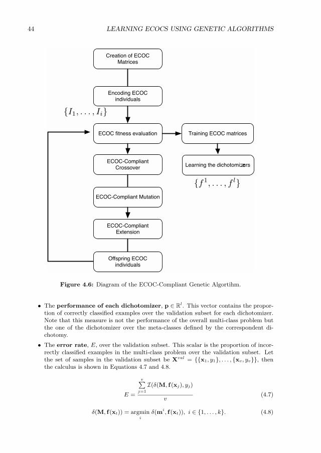
44 LEARNING ECOCS USING GENETIC ALGORITHMS

Creation of ECOC Matrices

Encoding ECOC individuals

ECOC-Compliant Crossover

ECOC-Compliant Mutation

ECOC-Compliant Extension

ECOC fitness evaluation Training ECOC matrices

Learning the dichotomizers

I1, . . . , Ii

f1, . . . , f l

Offspring ECOC individuals

Figure 4.6: Diagram of the ECOC-Compliant Genetic Algortihm.

• The performance of each dichotomizer, p ∈ Rl. This vector contains the propor-tion of correctly classified examples over the validation subset for each dichotomizer.Note that this measure is not the performance of the overall multi-class problem butthe one of the dichotomizer over the meta-classes defined by the correspondent di-chotomy.

• The error rate, E, over the validation subset. This scalar is the proportion of incor-rectly classified examples in the multi-class problem over the validation subset. Letthe set of samples in the validation subset be Xval = x1, y1, . . . , xv, yv, thenthe calculus is shown in Equations 4.7 and 4.8.

E =

v∑j=1I(δ(M, f(xj), yj)

v(4.7)

δ(M, f(xt)) = argmini

δ(mi, f(xt)), i ∈ 1, . . . , k. (4.8)

4.3. Learning ECOCs using ECOC-compliant Genetic Algorithms 45

• The decoding function, δ. We use the Loss-Weighted decoding [47] of Equation 4.9,where W ∈ Rk×l is a matrix of weights and L is a loss function (L(θ) = exp−θ in ourcase).

δLW (mi, f(x)) =l∑

j=1

wijL(mij · f j(x))) (4.9)

Fitness Function

The fitness function measures the adaptation of each individual, and thus, is the one to beoptimized. In this sense, the most common approach in state-of-the-art literature has beento evaluate an ECOC individual as the performance it obtains on the validation subset.Nevertheless, following Occam’s razor principles, in the hypothetical situation in which twoindividuals obtain the same performance on the field the one showing a simpler model (whichvery often implies a smaller code length) tends to be the most suitable choice.

This general assumption can be redefined and used in the fitness function in order topenalize those individuals with a large code length. Let I = I1, . . . , Ii be a a set ofindividuals and Ik a ECOC individual encoded as shown in Section 4.3.2, then our fitnessfunction is defined as shown in Equation 4.10.

F(Ik) = EIk + λlIk (4.10)

This expression (similar to the one showed by regularized classifiers), serve us to controlthe learning capacity and avoid over-fitting.

There exists several ways of defining complexity in the ECOC framework. Nevertheless,the code length has been always in the core of this definition. Thus, we have adopted theterm complexity as the number of dichotomies defined in the coding matrix M, that is l.

ECOC-Compliant Crossover and Mutation Operators

In this section we introduce the novel ECOC-compliant crossover and mutation operators.These operators do not only take into account the restrictions of the ECOC framework(shown in Equations 2.7, 2.8 and 2.9) but are also designed in order to avoid a prematureconvergence to local minima without generating non-valid individuals, and thus, convergingto satisfying results in fewer generations.

In our proposal, when performing the genetic optimization we have to take into accountthe effect of the operators used. In many Genetic Algorithms a trade-off between exploring asatisfying portion of the search space and converging quickly to a final population is desirable[70], thus avoiding the convergence to local minima. To achieve this goal in our proposaltwo versions of each operator were designed, the randomized and the biased. On one hand,the randomized version of each operator builds valid individuals with a random seed, whichaims to accomplish the exploration of a satisfying portion of the search space. On the otherhand, the biased version takes into account certain factors (i.e dichotomizer performances,confusion matrices, etc.) that imply the guidance of the optimization procedure to promisingregions of the search space, where individuals may obtain a better fitness value.• ECOC-Compliant Crossover AlgorithmIn GAs one of the most important issues is how individuals are recombined in order to

produce fitter offspring. In this sense, one would like to find an intelligent recombinationmethod (known as crossover operator) that take profit of problem domain information inorder to allow a faster convergence. Crossover operators are strongly defined for standard

46 LEARNING ECOCS USING GENETIC ALGORITHMS

GAs encodings schemes (such as binary encoding) and have been deeply studied in litera-ture. Nevertheless, when facing problems in which individuals are constrained and standardencoding designs have to be redefined, we consider also the redefinition of the recombinationprocedure to be an unavoidable task. This consideration is given by the fact that usingstandard GAs in problems where individuals are constrained can lead to situations wherethe search space is enlarged due to the generation of non-valid individuals.

Consider a k-class problem and let IF and IM be two individuals encoded as shown inSection 4.3.2. Then the crossover algorithm will generate a new individual IS which codingmatrix MIS ∈ −1, 0,+1k×l, l = min(MIF ,MIM ) contains dichotomies of each parent.Therefore, the key aspect of this recombination is the selection of which dichotomies ofeach parent are more suitable to be combined. Taking into account the aim of avoidingthe generation of non-valid individuals, we introduce a dichotomy selection algorithm thatchooses l dichotomies that fulfil the constraints shown in Equations 2.7, 2.8, and 2.9.

The dichotomy selection algorithm generates a dichotomy selection order t ∈ Nn for eachparent, where tI is the selection order of parent I and tIk is the value at the k-th position.However, this selection order can lead to a situation in which the l dichotomies chosen definean incongruence in the coding matrix, such as defining two classes with the same codeword.In such case, the dichotomy selection algorithm checks if the separation between codewordsis congruent with the number of dichotomies left to add.

Theorem 4.3.1 describes the number of equivalent codes allowed to appear on a matrixthat is being built to fulfil the ECOC properties in terms of rows (Equation 2.7). In thissense, when the final length of the ECOC matrix in terms of columns is known, we candetermine the maximum number of equivalent codes allowed to appear when each extensiondichotomy is appended to build the ECOC matrix.

Theorem 4.3.1 Should M ∈ −1, 0,+1k×l be a randomly distributed matrix. Then, theextension of Mk×l to an ECOC coding matrix M ∈ −1, 0,+1k×(l+l′) with k unequivocallydefined rows, will be possible if and only if when including the i-th (0 ≤ i ≤ l′) extensiondichotomy in M, 2(l′−i) repeated codewords of length t+ i are obtained at most.

Proof Let a matrix M ∈ −1, 0,+1k×l define Rl repeated codes (two codes mi,mj areequivalent if δAHD(mi,mj) = 0). Assume Mk×l is to be extended to Mk×(l+l′) so that itfulfills Equation 2.7: min(δAHD(mi,mj)) ≥ 1, ∀i, j : i 6= j, i, j ∈ [1, . . . , k].

Then, from Information theory dlog2(Rl)e is known to be the minimal number of ex-tension bits needed to unequivocally split Rl codes. Therefore, if Mk×l is extended with l′dichotomies, then dlog2(Rl)e ≤ l′ dichotomies are needed to assure that Equation 2.7 holds.When the first of the l′ dichotomies is added, then l′ − 1 dichotomies will be used to splitthe remaining set of repeated codes (Rl+1). As in the former case, dlog2(Rl+1)e ≤ l′ − 1are needed. Accordingly, when the second dichotomy is appended dlog2(Rl+2)e ≤ l′ − 2.Generalizing, Mk×l will only be extensible to a valid ECOC matrix Mk×l+l′ if when addingthe i-th dichotomy dlog2(Rl+i)e ≤ l′ − i. Thus, 2l

′−i repeated codewords are obtained atmost when adding the i-th extension dichotomy.

Following Theorem 4.3.1 the i-th dichotomy will be only added if it splits the existingcodewords to define Rl+i ≤ 2(l′−i) different codes. However, in a certain iteration it mayhappen that there are no existing dichotomies in both parents that accomplish the splitcriteria. In this situation, a new dichotomy is generated in order to ensure the ECOCproperties. We define the ECOC-compliant crossover algorithm as shown in Algorithm 1.

Two ECOC crossover algorithm variants are proposed, which have an equal probabilityof being executed. In the first one, which is the randomized version, the dichotomy selection

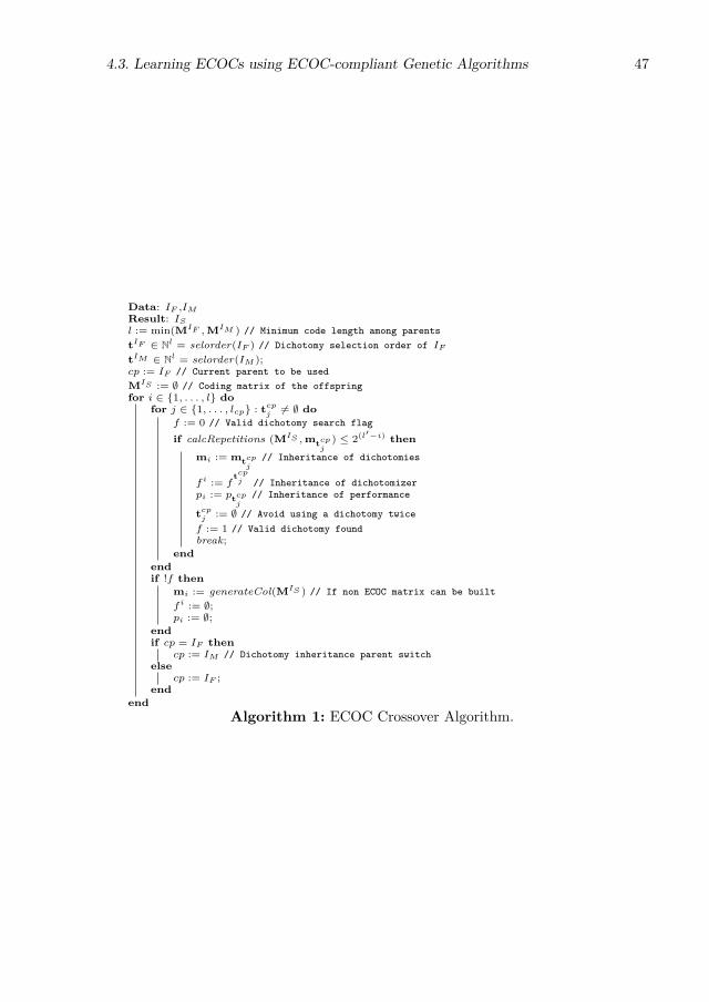
4.3. Learning ECOCs using ECOC-compliant Genetic Algorithms 47

Data: IF ,IM

Result: IS

l := min(MIF ,MIM ) // Minimum code length among parentstIF ∈ Nl = selorder(IF ) // Dichotomy selection order of IF

tIM ∈ Nl = selorder(IM );cp := IF // Current parent to be usedMIS := ∅ // Coding matrix of the offspringfor i ∈ 1, . . . , l do

for j ∈ 1, . . . , lcp : tcpj6= ∅ do

f := 0 // Valid dichotomy search flag

if calcRepetitions (MIS ,mtcpj

) ≤ 2(l′−i) then

mi := mtcpj

// Inheritance of dichotomies

fi := ftcp

j // Inheritance of dichotomizerpi := ptcp

j// Inheritance of performance

tcpj

:= ∅ // Avoid using a dichotomy twicef := 1 // Valid dichotomy foundbreak;

endendif !f then

mi := generateCol(MIS ) // If non ECOC matrix can be builtfi := ∅;pi := ∅;

endif cp = IF then

cp := IM // Dichotomy inheritance parent switchelse

cp := IF ;end

endAlgorithm 1: ECOC Crossover Algorithm.

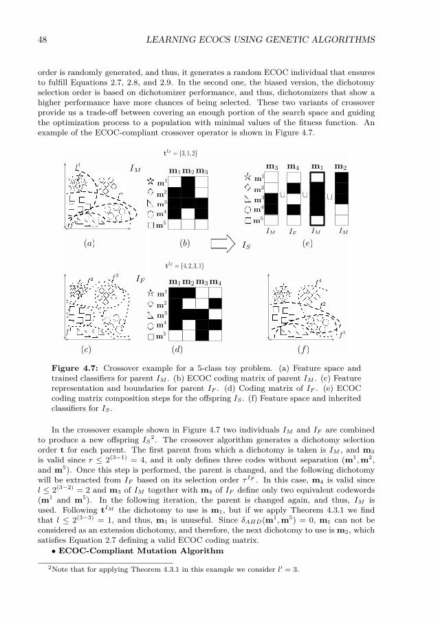
48 LEARNING ECOCS USING GENETIC ALGORITHMS

order is randomly generated, and thus, it generates a random ECOC individual that ensuresto fulfill Equations 2.7, 2.8, and 2.9. In the second one, the biased version, the dichotomyselection order is based on dichotomizer performance, and thus, dichotomizers that show ahigher performance have more chances of being selected. These two variants of crossoverprovide us a trade-off between covering an enough portion of the search space and guidingthe optimization process to a population with minimal values of the fitness function. Anexample of the ECOC-compliant crossover operator is shown in Figure 4.7.

(a)

f2

f1

f1

f4

f3

f2

(b)

(c)

tIF = 3, 1, 2

f3

tIF = 4, 2, 3, 1

∪ ∪ ∪

f4

f2

f3

(e)

(d)

IM

IF

IS

IM IF IM IM

(f)

m1

m2

m3

m4

m5

m1m2m3

m1

m2

m3

m4

m5

m1m2m3m4

m1

m2

m3

m4

m5

m3 m4 m1 m2

Figure 4.7: Crossover example for a 5-class toy problem. (a) Feature space andtrained classifiers for parent IM . (b) ECOC coding matrix of parent IM . (c) Featurerepresentation and boundaries for parent IF . (d) Coding matrix of IF . (e) ECOCcoding matrix composition steps for the offspring IS . (f) Feature space and inheritedclassifiers for IS .

In the crossover example shown in Figure 4.7 two individuals IM and IF are combinedto produce a new offspring IS2. The crossover algorithm generates a dichotomy selectionorder t for each parent. The first parent from which a dichotomy is taken is IM , and m3is valid since r ≤ 2(3−1) = 4, and it only defines three codes without separation (m1,m2,and m5). Once this step is performed, the parent is changed, and the following dichotomywill be extracted from IF based on its selection order τ IF . In this case, m4 is valid sincel ≤ 2(3−2) = 2 and m3 of IM together with m4 of IF define only two equivalent codewords(m1 and m5). In the following iteration, the parent is changed again, and thus, IM isused. Following tIM the dichotomy to use is m1, but if we apply Theorem 4.3.1 we findthat l ≤ 2(3−3) = 1, and thus, m1 is unuseful. Since δAHD(m1,m5) = 0, m1 can not beconsidered as an extension dichotomy, and therefore, the next dichotomy to use is m2, whichsatisfies Equation 2.7 defining a valid ECOC coding matrix.• ECOC-Compliant Mutation Algorithm

2Note that for applying Theorem 4.3.1 in this example we consider l′ = 3.

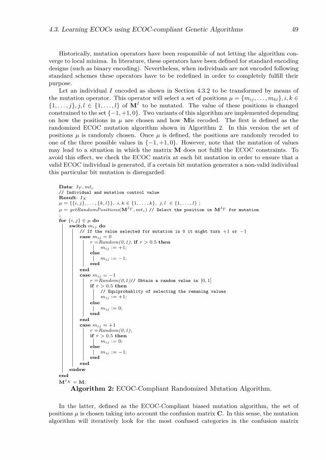
4.3. Learning ECOCs using ECOC-compliant Genetic Algorithms 49

Historically, mutation operators have been responsible of not letting the algorithm con-verge to local minima. In literature, these operators have been defined for standard encodingdesigns (such as binary encoding). Nevertheless, when individuals are not encoded followingstandard schemes these operators have to be redefined in order to completely fulfill theirpurpose.

Let an individual I encoded as shown in Section 4.3.2 to be transformed by means ofthe mutation operator. This operator will select a set of positions µ = mij , . . . ,mkl, i, k ∈1, . . . , j, j, l ∈ 1, . . . , l of MI to be mutated. The value of these positions is changedconstrained to the set −1,+1, 0. Two variants of this algorithm are implemented dependingon how the positions in µ are chosen and how Mis recoded. The first is defined as therandomized ECOC mutation algorithm shown in Algorithm 2. In this version the set ofpositions µ is randomly chosen. Once µ is defined, the positions are randomly recoded toone of the three possible values in −1,+1, 0. However, note that the mutation of valuesmay lead to a situation in which the matrix M does not fulfil the ECOC constraints. Toavoid this effect, we check the ECOC matrix at each bit mutation in order to ensure that avalid ECOC individual is generated, if a certain bit mutation generates a non-valid individualthis particular bit mutation is disregarded.

Data: IT ,mtc// Individual and mutation control valueResult: IX

µ = i, j, . . . , k, l, i, k ∈ 1, . . . , k, j, l ∈ 1, . . . , l ;µ = getRandomPositions(MIT ,mtc) // Select the position in MIT for mutation;for i, j ∈ µ do

switch mij do// If the value selected for mutation is 0 it might turn +1 or −1case mij = 0

r =Random(0,1); if r > 0.5 thenmij := +1;

elsemij := −1;

endendcase mij = −1

r =Random(0,1)// Obtain a random value in [0, 1]if r > 0.5 then

// Equiprobablity of selecting the remaning valuesmij := +1;

elsemij := 0;

endendcase mij = +1

r =Random(0,1);if r > 0.5 then

mij := 0;else

mij := −1;end

endendsw

endMIX = M;

Algorithm 2: ECOC-Compliant Randomized Mutation Algorithm.

In the latter, defined as the ECOC-Compliant biased mutation algorithm, the set ofpositions µ is chosen taking into account the confusion matrix C. In this sense, the mutationalgorithm will iteratively look for the most confused categories in the confusion matrix

50 LEARNING ECOCS USING GENETIC ALGORITHMS

i, j = argmaxi,j

cij + cji. Once these classes are obtained, the algorithm will transform

the bits valued 0 of codewords mi and mj in order to increase the distance δAHD(mi,mj),and thus, increasing their correction capability, while keeping a valid ECOC matrix. TheECOC-Compliant biased mutation algorithm is shown in Algorithm 3.

Data: IT ,mtc// Individual and mutation control valueResult: IX

CIT Rk×k // Confusion matrix of IT

ct := 0// Number of recoded bits of MIT

while ct < mtc doi, j := argmax

i,j

cij + cji ∀i, j : i 6= j;

for b ∈ 1, . . . , l doif |mib|+ |mjb| ≤ 1 and ct < mtc then

if mib = 0 and mjb = 0 thenmib := +1 // Invert both bits valued 0mjb := −1;

elseif mib = 0 then

mib := −mjb // Invert bit valued 0else

mjb := −mib;end

endct := ct + 1;

endendc

ITij

:= 0, cITji

:= 0;end

Algorithm 3: Biased ECOC-Compliant Mutation Algorithm.

In Figure 4.8 an example of the biased mutation algorithm is shown. Let IT be anindividual encoded as shown in Section 4.3.2. The confusion matrix CIT has its non-diagonalmaximum at c43 + c34. Then codewords m4 and m3 are going to be mutated. The 0valued bits of this codewords are changed in order to increment δAHD(m4,m3), and thus,incrementing also the correction capability between them. At the following iteration c43 isnot taken into consideration and the procedure will be repeated with m5 and m4 which arethe following classes that show confusion in C.

Problem-Dependent Extension of ECOCs

In related works that used GAs to optimize the ECOC matrices the length was fixed in acertain interval and the crossover operators where the ones responsible for obtaining reducedor large codes [62, 89]. Nevertheless, we consider that from the ECOC point of view thelength of the code is a crucial factor that has to be addressed separately, since the length ofthe code matrix has a direct relationship to its correction capability. In this sense, as statedin Section 4.3.2 our initial population is based on the coding scheme proposed by [10], thatis, the use of a Minimal ECOC coding matrix M ∈ −1, 0,+1k×dlog2(k)e. Nevertheless,when analyzing the Minimal ECOC matrix a lost of correction capability is found. Let Mbe a ECOC coding matrix, then:

ρ = min(δ(mi,mj)− 1

2

), ∀i, j ∈ 1, . . . , k, i 6= j. (4.11)

4.3. Learning ECOCs using ECOC-compliant Genetic Algorithms 51

(a) (b)

f2

f1

f3

MIT

0 3000

250 20

3 010 0

00 0 06

0006 0

(c)

CIT

f4

MIT

f2

f1

f3

f4

(d) (e)

m1

m2

m3

m4

m5

m1

m2

m3

m4

m5

c1

c2

c3

c4

c5

c1 c2 c3 c4 c5

m1m2m3m4

m1m2m3m4

Figure 4.8: Mutation example for a 5-class toy problem. (a) Feature space andtrained dichotomizers for and individual IT . (b) ECOC coding matrix of IT . (c)Confusion matrix of IT . (d) Mutated coding matrix. (e) Mutated feature space withtrained dichotomizers.

Therefore, we obtain a null correction capability ρ = 0 for the Minimal ECOC design,since for this ECOC matrices:

min(δAHD(mi,mj)∀i,j:i6=j) = 1, i, j ∈ [1, . . . , k]. (4.12)

This means that in Minimal ECOC coding schemes, a sample x will be misclassified if justa dichotomizer f i misses its prediction. Although this coding design has proved to be fairlyeffective when its properly tuned, we believe that an extension of such is needed to properlybenefit from Error-Correcting principles. However, this extension is not only motivated bythe null correction capability issue. The confusion between categories is also a determinantfactor when extending ECOC designs [48], since one would like to focus dichotomies in thosecategories which are more difficult to be learnt.

We propose a novel methodology to extend ECOC designs based on the confusion matrix,aiming to focus the extension dichotomies in those categories which are more difficult to belearnt, and thus, show a greater confusion. This methodology defines to types of extensions,the One vs. One extension and the Sparse extension, which have the same probability ofbeing executed along the optimization process. In the former, the ECOC coding matrixM ∈ −1, 0,+1k×l will be extended with a dichotomy ml+1 which will have 0 valuesexcept for those two positions mi and mj which correspond to the categories i, j thatmaximize the confusion i, j = argmax

i,j

cij + cji. In the second, the Sparsity Controlled

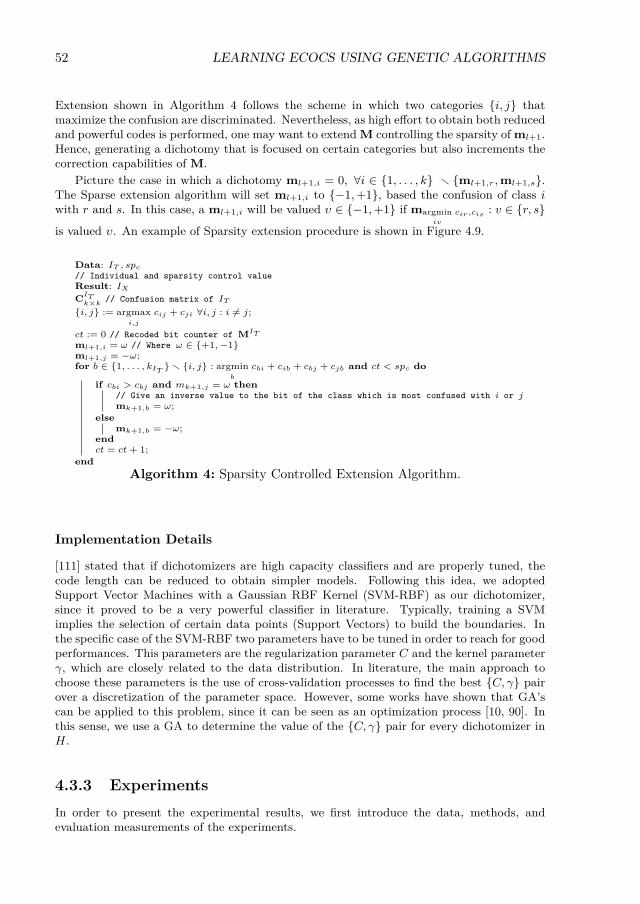
52 LEARNING ECOCS USING GENETIC ALGORITHMS

Extension shown in Algorithm 4 follows the scheme in which two categories i, j thatmaximize the confusion are discriminated. Nevertheless, as high effort to obtain both reducedand powerful codes is performed, one may want to extend M controlling the sparsity of ml+1.Hence, generating a dichotomy that is focused on certain categories but also increments thecorrection capabilities of M.

Picture the case in which a dichotomy ml+1,i = 0, ∀i ∈ 1, . . . , k r ml+1,r,ml+1,s.The Sparse extension algorithm will set ml+1,i to −1,+1, based the confusion of class iwith r and s. In this case, a ml+1,i will be valued υ ∈ −1,+1 if margmin

iv

cir,cis : v ∈ r, s

is valued υ. An example of Sparsity extension procedure is shown in Figure 4.9.

Data: IT , spc

// Individual and sparsity control valueResult: IX

CITk×k

// Confusion matrix of IT

i, j := argmaxi,j

cij + cji ∀i, j : i 6= j;

ct := 0 // Recoded bit counter of MIT

ml+1,i = ω // Where ω ∈ +1,−1ml+1,j = −ω;for b ∈ 1, . . . , kIT

r i, j : argminb

cbi + cib + cbj + cjb and ct < spc do

if cbi > cbj and mk+1,j = ω then// Give an inverse value to the bit of the class which is most confused with i or jmk+1,b = ω;

elsemk+1,b = −ω;

endct = ct + 1;

endAlgorithm 4: Sparsity Controlled Extension Algorithm.

Implementation Details

[111] stated that if dichotomizers are high capacity classifiers and are properly tuned, thecode length can be reduced to obtain simpler models. Following this idea, we adoptedSupport Vector Machines with a Gaussian RBF Kernel (SVM-RBF) as our dichotomizer,since it proved to be a very powerful classifier in literature. Typically, training a SVMimplies the selection of certain data points (Support Vectors) to build the boundaries. Inthe specific case of the SVM-RBF two parameters have to be tuned in order to reach for goodperformances. This parameters are the regularization parameter C and the kernel parameterγ, which are closely related to the data distribution. In literature, the main approach tochoose these parameters is the use of cross-validation processes to find the best C, γ pairover a discretization of the parameter space. However, some works have shown that GA’scan be applied to this problem, since it can be seen as an optimization process [10, 90]. Inthis sense, we use a GA to determine the value of the C, γ pair for every dichotomizer inH.

4.3.3 ExperimentsIn order to present the experimental results, we first introduce the data, methods, andevaluation measurements of the experiments.

4.3. Learning ECOCs using ECOC-compliant Genetic Algorithms 53

(a)(b)

f2

f1

f3

MIT

1 3100

250 20

3 010 0

00 0 16

0016 0

(c)

CIT

MIT

(d) (e)

f2

f1

f3

f4

m1

m2

m3

m4

m5

m1

m2

m3

m4

m5

m1m2m3m4

m1m2m3

c1

c2

c3

c4

c5

c1 c2 c3 c4 c5

Figure 4.9: Sparsity extension example for a 5-class toy problem. (a) Feature spaceand trained dichotomizers for IT . (b) ECOC coding matrix of IT . (c) Confusionmatrix of IT . (d) Extended coding matrix. (e) Extended feature space with traineddichotomizers.

Data

The data used on these experiments are the following UCI datasets [8]: Dermathology, Ecoli,Vehicle„ Segmentation, Glass, Vowel, Shuttle, Satimage, and Yeast.

In addition we performed experiments in four challenging Computer Vision datasets:Traffic Sign, ARface, Cleafs and Accidental, and MPEG7. Detailed descriptions and charac-teristics for each dataset can be found in Appendix A.

Methods

We compare the One vs. One [125] and One vs. All [111] ECOC, DECOC [106] and Forest-ECOC [49] approaches with the novel ECOC-compliant genetic approach. Moreover, theapproaches of Lorena et. al [89] and Pedrajas et. al [62] have been replicated in orderto obtain a fair comparison with state-of-the-art ECOC GA methods. The Loss-Weighteddecoding is applied at the decoding step [47]. The ECOC base classifier is the libsvmimplementation of SVM with Radial Basis Function kernel [29].

54 LEARNING ECOCS USING GENETIC ALGORITHMS

Experimental SettingsFor all experiments the base classifier used is an SVM with an RBF kernel. The optimiza-tion of its parameters is performed with a GA using a population of 60 individuals, usingthe operators defined by [10]. In addition for all evolutionary methods ([62], [89] and ourproposal), the number of ECOC individuals in the initial population is set to 5k, where k isthe number of classes of the problem. The elite individuals is set to 10% of the populationsize. The stopping criteria is a stall activity of performance results during five generations.

Evaluation MeasurementsThe classification performance is obtained by means of a stratified five-fold cross-validation,and tested for the confidence interval with a two-tailed t-test. We also apply the Fried-man and Nemenyi tests [38] in order to look for statistical significance among the obtainedperformances.

Experimental Classification ResultsThe classification results obtained for all the datasets considering the different ECOC con-figurations are shown in Table 4.2. The main trend of experimental results is that the Onevs. One coding is the most successful coding in terms of performance, obtaining very goodresults in most of the datasets. Nevertheless, in certain situations coding designs with farless number of dichotomizers can achieve similar or even better results (i.e Ecoli, Yeast, andCLEAFS results). Moreover, taking into account the number of classifiers yielded per eachcoding design we can see how those codings that were optimized with a GA are far more effi-cient than the predefined ones. In addition, in order to compare the performances providedfor each strategy, the table also shows the mean rank of each ECOC design considering the26 different experiments (13 classification accuracies and 13 coding lengths). The rankingsare obtained estimating each particular ranking rij for each problem i and each ECOC con-figuration j, and computing the mean ranking for each design as rj = 1

N

∑irji , where N is

the total number of datasets. We also show the mean number of classifiers (#) required foreach strategy. Furthermore, Table 4.3 shows the mean performance ranking and the mean

performance per classifier ranking, which is computed as the rank of PC =∑N

i=11−Ei∑N

i=1ni

,

where 1 − Ei is the performance obtained in the i-th problem and ni is the length of thecode in the i-th problem.

In order to reject the null hypothesis that the measured performance ranks differ fromthe mean performance rank, and that the performance ranks are affected by randomness inthe results, we use the Friedman test. The Friedman statistic value is computed as follows(following the notation of the seminal paper of Demsat et. al [38]):

X2F = 12N

k(k + 1)

[∑j

R2j −

k(k + 1)2

4

]. (4.13)

In our case, with k = 8 ECOC designs to compare, X2F = 11.26. Since this value is

undesirable conservative, Iman and Davenport proposed a corrected statistic:

FF = (N − 1)X2F

N(k − 1)−X2F

. (4.14)

Applying this correction we obtain FF = 1.1. With eight methods and thirteen experi-ments, FF is distributed according to the F distribution with 7 and 175 degrees of freedom.

4.3. Learning ECOCs using ECOC-compliant Genetic Algorithms 55

The critical value of F (7, 175) for 0.05 is 0.31. As the value of FF is higher than 0.31 we canreject the null hypothesis.

Furthermore, we perform a Nemenyi test in order to check if any of these methods canbe singled out [38], the Nemenyi statistic is obtained as follows:

CD = qα

√k(k + 1)

6N . (4.15)

In our case, for k = 8 ECOC designs to compare and N = 26 experiments the criticalvalue for a 90% of confidence is CD = 2.780 ·

√56

156 = 1.8. In this case, since our approach isthe best in rank but it intersects with Minimal ECOC, Pedrajas et. al, DECOC, and, Lorenaet al. approaches, we can state that there is no statistically significant difference among thesefive approaches. However, since our approach uses less dichotomizers than any of the otherapproaches (except for the Minimal ECOC which obtains the lowest classification accuracyranking) it can be considered as the most suitable choice.

Moreover, we have to take into account that although Binary Minimal ECOC, Pedrajaset. al, DECOC, and, Lorena et al. approaches intersect with our proposal, the number ofSVs defined by these approaches are generally bigger than the number of SVs defined by ourproposal. Therefore, their testing complexity is larger than the one showed by our method(see Section 4.3.4 for further details). As for the Minimal ECOC method, although the meanrank is close to our method we can see in Table 4.2 that the randomness of its optimizationleads to a much lower classification performance.

These results support our thesis of using far less dichotomizers than standard techniqueswhile searching for ECOC matrices with a extremely high efficiency. In addition, the generaltrend of the experiments shows that the proposed ECOC-Compliant GA improves the clas-sification accuracy of methods at the same complexity level and reduces the computationalcomplexity of methods with similar accuracy.

3 3.5 4 4.5 5 5.5 6

One vs. One

One vs. All

Forest ECOC

Lorena et. al.

DECOC

Pedrajas et. al

Minimal ECOC

ECOC−CompliantGA

CD 90%

Figure 4.10: Critical difference for the Nemenyi test and the performance per clas-sifier ranking values.

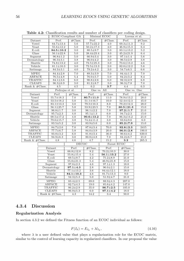
56 LEARNING ECOCS USING GENETIC ALGORITHMS

Table 4.2: Classification results and number of classifiers per coding design.ECOC-Compliant GA Minimal ECOC Lorena et al.

Dataset Perf. #Class. Perf. #Class. Perf. #Class.Vowel 64.7±13.4 5.6 57.7±22.2 4.0 69.3±11.3 9.2Yeast 55.6±12.2 5.0 50.2±17.3 4.0 46.9±15.3 6.4E.coli 84.5±10.2 3.0 80.5±9.7 3.0 83.1±13.2 5.2Glass 50.1±22.8 5.0 38.4±23.4 3.0 45.2±21.9 6.4

Segment 96.8±1.2 5.0 66.9±3.4 3.0 97.1±1.4 5.6Dermatology 96.3±3.1 3.8 96.0±4.2 3.0 96.5±2.9 3.8

Shuttle 74.8±13.2 4.0 72.5±25.3 3.0 73.6±13.2 4.6Vehicle 81.1±10.3 3.0 72.5±13.3 2.0 82.0±12.2 5.6Satimage 84.3±3.1 4.0 79.2±4.2 3.0 54.7±6.5 6.6MPEG 84.4±2.8 7.0 89.3±3.9 7.0 84.4±1.3 7.0

ARFACE 76.5±4.8 5.4 76.0±5.7 5.0 84.2±3.2 8.4TRAFFIC 84.1±3.6 6.0 90.8±2.6 6.0 92.3±2.9 6.8CLEAFS 96.3±6.9 3.0 81.2±8.7 3.0 96.3±7.8 7.0

Rank & #Class. 4.5 4.5 6.2 3.7 4.4 6.3Pedrajas et al. One vs. All One vs. One

Dataset Perf. #Class. Perf. #Class. Perf. #Class.Vowel 55.7±18.3 7.0 80.7±11.0 11.0 78.9±13.2 28.0Yeast 53.5±18.2 5.0 51.1±16.7 10.0 52.4±12.3 45.0E.coli 83.1±13.3 3.0 79.5±10.3 8.0 79.2±12.3 28.0Glass 56.1±25.7 5.0 53.9±23.5 7.0 60.5±21.3 15.0

Segment 96.8±1.7 3.0 96.1±2.2 7.0 97.2±1.7 21.0Dermatology 95.7±2.3 4.0 95.1±1.3 6.0 94.7±2.3 15.0

Shuttle 68.5±17.2 4.0 90.6±13.2 7.0 86.3±14.2 21.0Vehicle 79.6±15.7 3.8 74.2±11.2 3.0 83.6±9.6 6.0Satimage 83.5±5.2 3.0 83.9±5.6 6.0 85.2±7.9 15.0MPEG 84.7±2.6 7.0 87.8±3.4 70.0 92.8±2.3 2415

ARFACE 77.7±6.7 5.8 84.0±3.9 20.0 96.0±2.8 190.0TRAFFIC 93.8±3.2 6.0 91.8±3.4 36.0 90.6±4.2 630.0CLEAFS 94.9±6.3 3.0 80.8±4.8 7.0 84.2±6.7 21.0

Rank & #Class. 4.8 4.6 4.7 15.2 3.2 265.3DECOC Forest ECOC

Dataset Perf. #Class. Perf. #Class.Vowel 66.8±12.8 8.2 70.2±10.3 30.0Yeast 55.8±15.4 5.4 56.1±13.2 27.0E.coli 69.5±9.7 4.2 75.2±8.9 21.0Glass 55.0±21.3 5.4 46.9±21.8 15.0

Segment 97.0±2.3 4.6 97.1±1.3 18.0Dermatology 97.1±4.3 2.8 96.0±2.1 15.0

Shuttle 77.1±13.2 3.6 84.4±12.1 18.0Vehicle 84.1±10.3 4.6 81.7±13.3 9.0Satimage 52.3±5.3 5.0 51.9±4.7 21.0MPEG 83.4±2.5 69.0 88.9±4.3 207.0

ARFACE 82.7±4.3 19.0 85.6±4.2 147.0TRAFFIC 86.2±2.9 35.0 96.7±2.5 105.0CLEAFS 96.9±5.3 6.0 97.1±4.2 18.0

Rank & #Class. 4.3 14.2 3.4 50.0

4.3.4 DiscussionRegularization Analysis

In section 4.3.2 we defined the Fitness function of an ECOC individual as follows:

F (Ik) = EIk + λlIk , (4.16)

where λ is a user defined value that plays a regularization role for the ECOC matrix,similar to the control of learning capacity in regularized classifiers. In our proposal the value

4.3. Learning ECOCs using ECOC-compliant Genetic Algorithms 57

Table 4.3: Mean rank per coding design.ECOC-Compliant GA Minimal ECOC Lorena et al. Pedrajas et al.

Perf. rank 4.5 6.2 4.4 4.8#Class. rank 2 1 5 3

PC rank 3.2 3.6 4.7 3.9One vs.All ECOC One vs. One ECOC DECOC Forest ECOC

Perf. rank 4.7 3.2 4.3 3.4#Class. rank 6 8 4 7

PC rank 5.3 5.6 4.1 5.2

of λ is estimated by a cross-validation procedure. In Figure 4.11 a cross-validation procedureto determine the λ value is shown for the Vowel dataset. In this procedure, the values of λfollow a logarithmic progression (from 0.01 to 1). It can be seen how the number of classifiersyielded by the proposal diminishes when λ increases (particularly between 0.01 and 0.05).Finding its minimum at λ = 0.06 which corresponds to the Minimal ECOC length [10].

In this sense, in our experimental settings the lambda value was set to be in the middlepoint of the interval [λmin, λmax], where λmin is the smallest value of λ that yielded thesmallest ECOC code length, and respectively for λmax. Therefore, by performing this cross-validation setting of λ our proposal is able to find accurate models without a extremely highcomplexity in terms of the number of classifiers.

Complexity Analysis

In order to provide a complete description of the method, in this section we analyze itscomputational training and testing cost.

Let us consider the average computational cost for optimizing a dense dichotomizer (adichotomizer in which all classes are taken into account) as a constant value. Then we findthat in the case of One vs. All coding, we have k dichotomizers to be optimized, and thus, itscomputational cost is O(k). In the case of evolutionary codings (Pedrajas et al., Lorena et al.and our proposal) we have O(G · I · log2(k)), where I represents the number of individuals inthe genetic optimization (which is constant along generations) and G represents the numberof generations of the Genetic Algorithm. Undoubtedly, this cost may be greater than the costof the other non evolutionary techniques. Nevertheless, with the introduction of a cache ofoptimized dichotomizers each dichotomizer is optimized once and its parameters are storedfor future usage. In this sense, since the number of partitions of the classes is finite, as thealgorithm progresses, the number of dichotomizers to be optimized exponentially decreases.Thus, with this approximation procedure the value of G tends to one. In consequence, in anoptimal case the computational complexity becomes O(I · log2(k)).

In addition to the usual performance measures we also provide the number of SupportVectors (SVs) per coding scheme. Since this number is proportional to the complexity inthe test step we can perform an analysis of what strategies show less complexity while stillobtaining high performance. Figure 4.11(b) shows the number of SVs per coding design forthe UCI data and Figure 4.11(b) shows the number of SVs for the Computer Vision problems.We can see that, in most cases, the four first columns of each dataset (corresponding to theBinary Minimal and all the evolutionary strategies) yield a lower number of SVs per model.Analyzing the empirical results shown in Figures 4.12 and 4.11(b), we find that the numberof SVs defined by all three evolutionary strategies and the Binary Minimal approach aresignificantly smaller than the number of SVs defined by other strategies. This is due tothe fact that all initial populations of evolutionary methods were set to follow a Minimaldesign [10], and thus, they are all expected to yield a similar number of SVs. However,

58 LEARNING ECOCS USING GENETIC ALGORITHMS

0 0.01 0.04 0.06 0.08 0.1 0.2 0.4 0.6 0.8 10

1

2

3

4

5

6

7

8

9

10

λ value

#C

lassifie

rs

(a)

MPEG ARFACE TRAFFIC CLEAFS0

0.5

1

1.5

2

2.5

3

3.5

4

4.5

5x 10

4

ECOC−Compliant GA

Minimal ECOC

Lorena et. al.

Pedrajas et. al.

One vs. All

One vs. One

DECOC

Forest ECOC

(b)

Figure 4.11: (a) Number of classifiers per λ value on the UCI Vowel dataset. (b)Number of SVs per coding design in the Computer Vision problems.

the new proposal defines a more reduced number of SVs than other standard predefinedor even problem-dependent strategies. Defining a compact but yet discriminate enoughnumber of SVs, obtaining comparable or even better results than other coding designs whiledramatically reducing the testing time.

4.3. Learning ECOCs using ECOC-compliant Genetic Algorithms 59

Vowel Yeast E.Coli Glass Segmentation Dermatology Shuttle Vehicle Satimage0

500

1000

1500

2000

2500

3000

ECOC−Compliant GA

Minimal ECOC

Lorena et. al.

Pedrajas et. al.

One vs. All

One vs. One

DECOC

Forest ECOC

Figure 4.12: Number of SVs per coding design in the UCI datasets.

Convergence Analysis

This section is devoted to perform an analysis of convergence for the methods that use aGA to optimize the ECOC matrix ([62, 89] and our proposal). To properly perform thisanalysis we ran experiments for three UCI datasets (Glass, Vowel and Yeast), fixing theinitial population to avoid the random initialization point issue (although equivalent ECOCmatrices may yield different results due to the Genetic tuning of the SVM parameters). Thenumber of generations was set to 50 and the rest of the experimental settings were the sameas the ones described in Section 4.3.3.

In Figure 5.2 we show the evolution of the classification error, as well as the evolution ofthe performance per classifier rate for three UCI datasets. In Figures 5.2(a), 5.2(c) and 5.2(e)we can see how most of the times our proposal converges faster to better results than thestate-of-the-art GA approaches. This fact is motivated by the redefinition of the operatorsthat allows a fast exploration of the search space, without generating non-valid individuals.In addition, Figures 5.2(b), 5.2(d) and 5.2(f) show the evolution of the performance perclassifier rate along generations. Figures 5.2(b) and 5.2(f) clearly show that our proposalyields models that are more efficient since we get a higher performance per classifier rate.Nevertheless, in Figure 5.2(d) the proposal of Pedrajas et al. obtains a higher rate. This ismotivated by the fact that in the calculus of such rate both the classification error and theproduced code length have the same weight. However, Figure 5.2(c) clearly shows that ourmethod obtains better classification results.

Experimental results show that our proposal is able to converge faster to better results.In addition, the models yielded by the novel proposal are more efficient than the ones ob-tained by similar approaches. These results are obtained because of the redefinition of thecrossover and mutation operators taking into account the theoretical properties of the ECOCframework. In this sense, our operators have a higher probability of finding good ECOC ma-trices than others since our search space is more reduced and the operators can guide theoptimization procedure to promising regions of the search space.

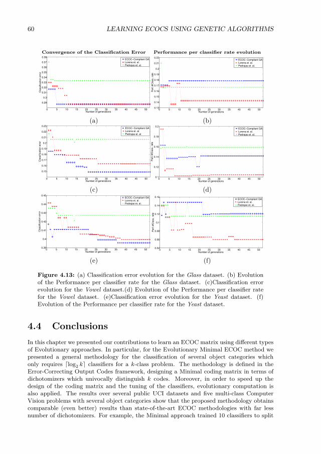
60 LEARNING ECOCS USING GENETIC ALGORITHMS

Convergence of the Classification Error Performance per classifier rate evolution

0 5 10 15 20 25 30 35 40 45 50

0.29

0.3

0.31

0.32

0.33

0.34

0.35

0.36

0.37

0.38

Number of generations

Cla

ssific

ation e

rror

ECOC−Compliant GALorena et. al.Pedrajas et. al.

0 5 10 15 20 25 30 35 40 45 500.13

0.14

0.15

0.16

0.17

0.18

0.19

0.2

0.21

0.22

Number of generations

Perf

./#C

lass. ra

te

ECOC−Compliant GALorena et. al.Pedrajas et. al.

(a) (b)

0 5 10 15 20 25 30 35 40 45 50

0.15

0.16

0.17

0.18

0.19

0.2

0.21

0.22

0.23

Number of generations

Cla

ssific

ation e

rror

ECOC−Compliant GALorena et. al.Pedrajas et. al.

0 5 10 15 20 25 30 35 40 45 500.1

0.12

0.14

0.16

0.18

0.2

Number of generations

Perf

./#C

lass. ra

te

ECOC−Compliant GALorena et. al.Pedrajas et. al.

(c) (d)

0 5 10 15 20 25 30 35 40 45 500.39

0.4

0.41

0.42

0.43

0.44

0.45

Number of generations

Cla

ssific

ation e

rror

ECOC−Compliant GALorena et. al.Pedrajas et. al.

0 5 10 15 20 25 30 35 40 45 500.04

0.06

0.08

0.1

0.12

0.14

0.16

Number of generations

Perf

./#C

lass. ra

te

ECOC−Compliant GALorena et. al.Pedrajas et. al.

(e) (f)

Figure 4.13: (a) Classification error evolution for the Glass dataset. (b) Evolutionof the Performance per classifier rate for the Glass dataset. (c)Classification errorevolution for the Vowel dataset.(d) Evolution of the Performance per classifier ratefor the Vowel dataset. (e)Classification error evolution for the Yeast dataset. (f)Evolution of the Performance per classifier rate for the Yeast dataset.

4.4 ConclusionsIn this chapter we presented our contributions to learn an ECOC matrix using different typesof Evolutionary approaches. In particular, for the Evolutionary Minimal ECOC method wepresented a general methodology for the classification of several object categories whichonly requires dlog2 ke classifiers for a k-class problem. The methodology is defined in theError-Correcting Output Codes framework, designing a Minimal coding matrix in terms ofdichotomizers which univocally distinguish k codes. Moreover, in order to speed up thedesign of the coding matrix and the tuning of the classifiers, evolutionary computation isalso applied. The results over several public UCI datasets and five multi-class ComputerVision problems with several object categories show that the proposed methodology obtainscomparable (even better) results than state-of-the-art ECOC methodologies with far lessnumber of dichotomizers. For example, the Minimal approach trained 10 classifiers to split

4.4. Conclusions 61

184 face categories, meanwhile the one-versus-all and one-versus-one approaches required184 and 16836 dichotomizers, respectively.

Furthermore, we observed that operators for standard GA encoding fail to take into ac-count the properties of ECOC matrices and their structure. Thus, we proposed to redefinethe crossover and mutation operators to avoid the massive generation of non-valid individ-uals. Specifically, we presented a novel ECOC-Compliant Genetic Algorithm for the codingstep in the ECOC framework. The proposed methodology redefines the usual crossover andmutation operators taking into account the properties of ECOC matrices. As a result, thesearch space is cropped, which causes the optimization to converge faster. Furthermore, anew operator which is able to increment the code length in a smart way was also introduced.The initial ECOC population followed a Minimal coding scheme, in which only dlog2(k)eclassifiers are needed to discriminate k classes, and as consequence, the methodology is ableto find very efficient codes.

The ECOC-Compliant GA was tested on a wide set of datasets of the UCI MachineLearning Repository and over four challenging Computer Vision problems. For comparisonpurposes state-of-the-art ECOC GA schemes were replicated, as well as standard ECOCcoding techniques. All the experiments were carried out using Support Vector Machineswith an RBF kernel. Experimental results showed that the new proposal obtains significantimprovements in comparison to state-of-the-art techniques. In particular, we analyzed theperformance in terms of code length, and training and testing complexity. Those analysisshowed that our proposal is able to find ECOC matrices with a high efficiency based on atrade-off optimization between performance and complexity obtained along the GA ECOC-Compliant optimization process.

62 LEARNING ECOCS USING GENETIC ALGORITHMS

Chapter 5

Learning ECOCs via theError-Correcting Factorization

Problem-dependent ECOC designs in literature have always focused on the column pictureof the ECOC matrix, that is, on the design of the binary problems which are coupled inthe ECOC coding design. In order to look for the more suitable binary problems, severalalgorithms have been applied with successful results [49, 60, 62, 106, 141] and in previouschapters of this thesis we presented our contribution using GAs. However, we consider thatanalyizing the row picture (i.e. the distance between codewords) can shed more interestingresults to analyze the Error-Correcting properties of an ECOC design, and yet surprisinglyhas not been exploited yet.

In this chapter, we present the Error-Correcting Factorization (ECF) method for factor-izing a design matrix D ∈ Rk×k of desired ’error-correcting properties’ between classes intoa discrete ECOC matrix. The proposed ECF method is a general framework for the ECOCcoding step since the design matrix is a flexible tool for error-correction analysis. In thissense, the problem of designing the ECOC matrix is reduced to defining the design matrix,where higher level reasoning may be used. For example, following recent state-of-the-artworks one could build a design matrix following a "hard classes are left behind" spirit, boost-ing the boundaries of easily separable classes and disregarding the classes that are not easilyseparable. An alternative for building the design matrix is the "no class is left behind" crite-ria, where we may boost those classes that are prone to be confused in the hope of recoveringmore errors. Note that the design matrix could also directly encode knowledge of domainexperts on the problem, providing a great flexibility on the design of the ECOC coding ma-trix. In addition, by using the Design matrix we derive the optimal problem-dependent codelength for ECOCs obtained by means of ECF, which to the best of our knowledge is the firsttime this question is tackled in the extended ECOC literature. In addition, we show howECF converges to a solution with negligible objective value when the design matrix followscertain constraints.

5.1 Error-Correcting FactorizationWe propose to cast the ECOC coding matrix optimization as a Matrix Factorization problemthat can be solved efficiently using a constrained coordinate descent approach. This sectiondescribes the objective function and the optimization strategy for the ECF algorithm.

63

64 LEARNING ECOCS VIA THE ERROR-CORRECTING FACTORIZATION

5.1.1 ObjectiveOur goal is to find an ECOC coding matrix that encodes the properties denoted by thedesign matrix D. In this sense, ECF seeks a factorization of the design matrix D ∈ Rk×kinto a discrete ECOC matrix M ∈ −1,+1k×l. This factorization is formulated as thequadratic form MM> that reconstructs D with minimal Frobenius distance under severalconstraints, as shown in Equation (5.1) 1.

minimizeM

‖D−MM>‖2F (5.1)

subject to M ∈ −1,+1k×l (5.2)MM> −P ≤ 0 (5.3)M>M− 1(l − 1) ≤ 0 (5.4)−M>M− 1(l − 1) ≤ 0 (5.5)

The component M ∈ −1,+1k×l that solves this optimization problem generates theinner product of discrete vectors that is closest to D under the Frobenius norm. In order forM to be a valid matrix under the ECOC framework we constraint M in Equations (5.2)-(5.5). Equation (5.2) ensures that each binary problem classes will belong to one of the twopossible meta-classes. In addition, to avoid the case of having two or more equivalent rowsin M, the constraints in 5.3 ensure that the correlation between rows of M less or equalthan a certain user-defined matrix −1l ≤ P ≤ 1l (recall that 1 denotes a matrix or vector ofall 1s of the appropriate size when used), where P encodes the minimum distance betweenany pair of codewords. P is a symmetric matrix with pii = l ∀i. Thus, by setting the offdiagonal values in P we can control the minimum inter-class correction capability. Hence, ifwe want the correction capability of rows mi and mj to be b c−1

2 c, we set pi = pj = 1(l− c).Finally, constraints in Equations (5.4) and (5.5) ensure the induced binary problems are

not equivalent. Similar constraints have been studied thoroughly in literature [39, 62, 84]defining methods that rely on diversity measures for binary problems to obtain a codingmatrix M. Equations (5.4) and (5.5) can be considered as soft-constraints since its violationdoes not imply violating the ECOC properties in terms of row distance. This is easy to showsince a coding matrix M ∈ −1,+1k×l that induces some equivalent binary problems butensures that MM> ≤ 1(l−1), ∀i, j : i 6= j will define a matrix whose rows are unequivocallydefined. In this sense, a coding matrix M can be easily projected on the set defined byconstraints (5.4) and (5.5) by eliminating repeated columns, M = mj : mj 6= mi∀j 6= i.Thus, constraints in 5.4 and 5.5 ensure that uncorrelated binary sub-problems will be definedin our coding matrix M. The discrete constraint in Equation 5.2 on the variable elevates theoptimization problem to the NP-Hard class. To overcome this issue and following [20, 32, 142]we relax the discrete constraint in 5.2 an replace it by M ∈ [−1,+1]k×l in Equation 5.7.

5.1.2 OptimizationIn this section, we detail the process for optimizing M. The minimization problem posed inEquation (5.1) with the relaxation of the boolean constraint in Equation (5.2) is non-convex,thus, M∗ is not guaranteed to be a global minimum. In this sense, although gradient de-scent techniques have been successfully applied in the literature to obtain local minimums[2, 83, 112] these techniques do not enjoy the efficiency and scalability properties present inother optimization methods applied to Matrix Factorization problems, such as Coordinate

1Recall that the l1 distance is a function of the dot product ‖mi −mj‖1 = −(mimj>)+l2 .

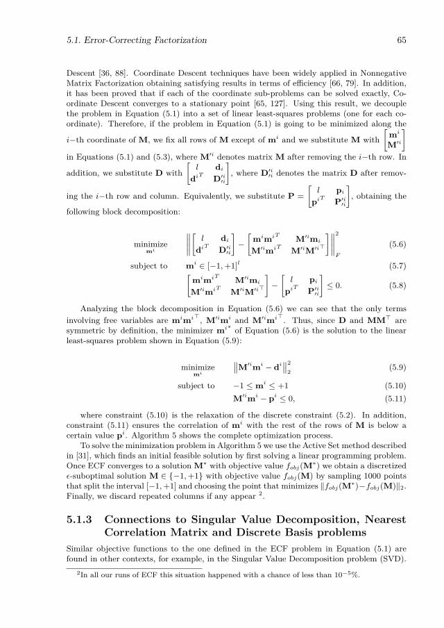
5.1. Error-Correcting Factorization 65

Descent [36, 88]. Coordinate Descent techniques have been widely applied in NonnegativeMatrix Factorization obtaining satisfying results in terms of efficiency [66, 79]. In addition,it has been proved that if each of the coordinate sub-problems can be solved exactly, Co-ordinate Descent converges to a stationary point [65, 127]. Using this result, we decouplethe problem in Equation (5.1) into a set of linear least-squares problems (one for each co-ordinate). Therefore, if the problem in Equation (5.1) is going to be minimized along the

i−th coordinate of M, we fix all rows of M except of mi and we substitute M with[

mi

M′i

]in Equations (5.1) and (5.3), where M′i denotes matrix M after removing the i−th row. In

addition, we substitute D with[l di

diT D′i′i

], where D′i′i denotes the matrix D after remov-

ing the i−th row and column. Equivalently, we substitute P =[l pi

piT P′i′i

], obtaining the

following block decomposition:

minimizemi

∥∥∥∥[ l didiT D′i′i

]−[

mimiT M′imi

M′imiT M′iM′i>

]∥∥∥∥2

F

(5.6)

subject to mi ∈ [−1,+1]l (5.7)[mimiT M′imi

M′imiT M′iM′i>

]−[l pi

piT P′i′i

]≤ 0. (5.8)

Analyzing the block decomposition in Equation (5.6) we can see that the only termsinvolving free variables are mimi>, M′imi and M′imi>. Thus, since D and MM> aresymmetric by definition, the minimizer mi∗ of Equation (5.6) is the solution to the linearleast-squares problem shown in Equation (5.9):

minimizemi

∥∥M′imi − di∥∥2

2(5.9)

subject to −1 ≤mi ≤ +1 (5.10)M′imi − pi ≤ 0, (5.11)

where constraint (5.10) is the relaxation of the discrete constraint (5.2). In addition,constraint (5.11) ensures the correlation of mi with the rest of the rows of M is below acertain value pi. Algorithm 5 shows the complete optimization process.

To solve the minimization problem in Algorithm 5 we use the Active Set method describedin [31], which finds an initial feasible solution by first solving a linear programming problem.Once ECF converges to a solution M∗ with objective value fobj(M∗) we obtain a discretizedε-suboptimal solution M ∈ −1,+1 with objective value fobj(M) by sampling 1000 pointsthat split the interval [−1,+1] and choosing the point that minimizes ‖fobj(M∗)−fobj(M)‖2.Finally, we discard repeated columns if any appear 2.

5.1.3 Connections to Singular Value Decomposition, NearestCorrelation Matrix and Discrete Basis problems

Similar objective functions to the one defined in the ECF problem in Equation (5.1) arefound in other contexts, for example, in the Singular Value Decomposition problem (SVD).

2In all our runs of ECF this situation happened with a chance of less than 10−5%.

66 LEARNING ECOCS VIA THE ERROR-CORRECTING FACTORIZATION

Data: D ∈ Rk×k,P ∈ Nk×k, lResult: M ∈ −1,+1k×lbegin

repeatforeach i ∈ 1, 2, . . . , k do

mi ← minimizemi∈Rl

∥∥M′imi − di∥∥2

2 , subject to : −1 ≤mi ≤

+1, M′imi − pi ≤ 0;endM← ε-suboptimal(M);M = mj : mj 6= mi∀j 6= i; // Projection step to removeduplicate columns

until convergence;end

Algorithm 5: Error-Correcting Factorization Algorithm.

The SVD uses the same objective function as ECF subjected to the constraint MM> = I.However, the solution of SVD yields an orthogonal basis, disagreeing with the objectivedefined in Equation (5.1) which ensures different correlations between the mi’s. In addition,we can also find a common ground with the Nearest Correlation Matrix (NMC) Problem[21, 69, 93]. However, the NMC solution does not yield a discrete factor M, instead it seeksdirectly for the Gramian MM> where M is not discrete, as in Equation (5.12).

minimizeM

‖M−D‖2F (5.12)

subject to M 0 (5.13)cMc> = b (5.14)

In addition, the ECF has similarities with the Discrete Basis Problem (DBP) [96], sincethe factors are M discrete valued. Nevertheless, DBP factorizes D ∈ 0, 1k×k instead ofD ∈ Rk×k, as show in Equation (5.15).

minimizeM,Y

‖M Y−D‖1 (5.15)

subject to M,Y,D ∈ 0, 1 (5.16)

5.1.4 Ensuring a representable design matrixAn alternative interpretation for ECF is that it seeks for a discrete matrix M whose Gramianis closest to D under the Frobenius norm. However, since D can be directly set by the userwe need to guarantee that D is a correlation matrix that is realizable in the Rk×k space, thatis, D has to be symmetric and positive semi-definite. In particular, we would like to find thecorrelation matrix D ∈ Rk×k that is closest to D under the Frobenius norm. This problemhas been treated in several works [21, 28, 63, 69], resulting in various algorithms that oftenuse an alternating projections approach. However, for this particular case in addition to bein the Positive Semidefinite (PSD) Cone and symmetric we also require D to be scaled in the[−l,+l] range, with δii = l∀i. In this sense, to find D we follow an alternating projections

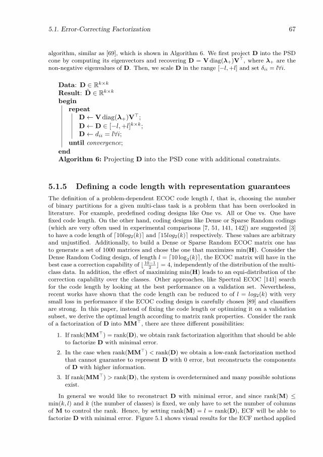
5.1. Error-Correcting Factorization 67

algorithm, similar as [69], which is shown in Algorithm 6. We first project D into the PSDcone by computing its eigenvectors and recovering D = V diag(λ+)V>, where λ+ are thenon-negative eigenvalues of D. Then, we scale D in the range [−l,+l] and set δii = l∀i.

Data: D ∈ Rk×kResult: D ∈ Rk×kbegin

repeatD← V diag(λ+)V>;D← D ∈ [−l,+l]k×k;D← dii = l∀i;

until convergence;endAlgorithm 6: Projecting D into the PSD cone with additional constraints.

5.1.5 Defining a code length with representation guaranteesThe definition of a problem-dependent ECOC code length l, that is, choosing the numberof binary partitions for a given multi-class task is a problem that has been overlooked inliterature. For example, predefined coding designs like One vs. All or One vs. One havefixed code length. On the other hand, coding designs like Dense or Sparse Random codings(which are very often used in experimental comparisons [7, 51, 141, 142]) are suggested [3]to have a code length of d10log2(k)e and d15log2(k)e respectively. These values are arbitraryand unjustified. Additionally, to build a Dense or Sparse Random ECOC matrix one hasto generate a set of 1000 matrices and chose the one that maximizes min(H). Consider theDense Random Coding design, of length l = d10 log2(k)e, the ECOC matrix will have in thebest case a correction capability of b 10−1

2 c = 4, independently of the distribution of the multi-class data. In addition, the effect of maximizing min(H) leads to an equi-distribution of thecorrection capability over the classes. Other approaches, like Spectral ECOC [141] searchfor the code length by looking at the best performance on a validation set. Nevertheless,recent works have shown that the code length can be reduced to of l = log2(k) with verysmall loss in performance if the ECOC coding design is carefully chosen [89] and classifiersare strong. In this paper, instead of fixing the code length or optimizing it on a validationsubset, we derive the optimal length according to matrix rank properties. Consider the rankof a factorization of D into MM>, there are three different possibilities:

1. If rank(MM>) = rank(D), we obtain rank factorization algorithm that should be ableto factorize D with minimal error.

2. In the case when rank(MM>) < rank(D) we obtain a low-rank factorization methodthat cannot guarantee to represent D with 0 error, but reconstructs the componentsof D with higher information.

3. If rank(MM>) > rank(D), the system is overdetermined and many possible solutionsexist.

In general we would like to reconstruct D with minimal error, and since rank(M) ≤min(k, l) and k (the number of classes) is fixed, we only have to set the number of columnsof M to control the rank. Hence, by setting rank(M) = l = rank(D), ECF will be able tofactorize D with minimal error. Figure 5.1 shows visual results for the ECF method applied

68 LEARNING ECOCS VIA THE ERROR-CORRECTING FACTORIZATION

D D

(a) (b)XX⊤ XX>

(c) (d)

Figure 5.1: D matrix for the Traffic (a) and ARFace (b) datasets. MM> termobtained via ECF for Traffic (c) and ARFace (d) datasets. ECOC coding matrix Mobtained with ECF for Traffic (e) and ARFace (f).

on the Traffic and ARFace datasets. Note how, for the Traffic (36 classes) and ARFaces(50 classes) datasets the required code length for ECF to full rank factorization is l = 6 andl = 8, respectively as shown in Figures 5.1(e)(f).

5.1.6 Order of Coordinate UpdatesCoordinate Descent has been applied in a wide span of problems obtaining satisfying results.However, the problem of choosing the coordinate to minimize at each iteration still remainsactive [58, 71, 110, 127]. In particular, [99] derives a convergence rate which is faster whencoordinates are chosen uniformly at random rather than on a cyclic fashion. Hence, choosingcoordinates at random its a suitable choice when the problem shows some of the followingcharacteristics [110]:

• Not all data is available at all times.• A randomized strategy is able to avoid worst-case order of coordinates, and hence

might be preferable.• Recent efforts suggest that randomization can improve the convergence rate [99].

5.1. Error-Correcting Factorization 69

However, the structure of ECF is different and calls for a different analysis. In particular,we remark the following points. (i) At each coordinate update of ECF, information aboutthe rest of coordinates is available. (ii) Since our coordinate updates are solved uniquely, arepetition on a coordinate update does not change the objective function. (iii) The descenton the objective value when updating a coordinate is maximal when all other coordinateshave been updated. These reasons leads us to choose a cyclic update scheme for ECF. Inaddition in Figure 5.2 we show a couple of examples in which the cyclic order of coordinatesconverges faster than the random order for two problems: Vowel and ARFace (refer to Section5.2 for further information on the datasets). This behavior is common for all datasets. Inparticular, note how the cyclic order of coordinates reduces the standard deviation on theobjective function, which is denoted by the narrower blue shaded area in Figure 5.2.

(a) (b)

Figure 5.2: Mean Frobenius norm value with standard deviation as a functionof the number of coordinate updates on 50 different trials. The blue shaded areacorresponds to cyclic update while the red area denotes random coordinate updatesfor Vowel (a) and ARFAce (b) datasets.

5.1.7 Approximation Errors and Convergence results when Dis an inner product of binary data

The optimization problem posed by ECF in Equation (5.1) is non-convex due to the quadraticterm MM>, even if the discrete constraint is relaxed. This implies that we cannot guaranteethat the algorithm converges to the global optima. Recall that ECF seeks for the term MM>

that is closest to D under the Frobenius norm. Hence, the error in the approximation canbe measured by ‖M∗M∗> −D‖2

F ≥ 0, where M∗ is the local optimal point to which ECFconverges. In this sense, we introduce DB which is the matrix of inner products of discretevectors that is closest to D under the Frobenious norm. Thus, we expand the norm as inthe following equation:

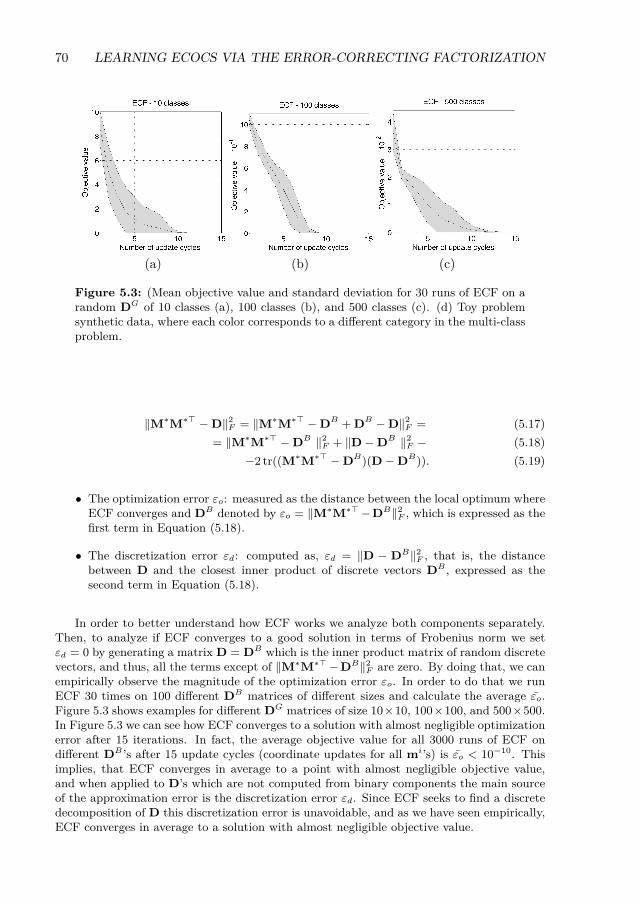
70 LEARNING ECOCS VIA THE ERROR-CORRECTING FACTORIZATION

(a) (b) (c)

Figure 5.3: (Mean objective value and standard deviation for 30 runs of ECF on arandom DG of 10 classes (a), 100 classes (b), and 500 classes (c). (d) Toy problemsynthetic data, where each color corresponds to a different category in the multi-classproblem.

‖M∗M∗> −D‖2F = ‖M∗M∗> −DB + DB −D‖2

F = (5.17)= ‖M∗M∗> −DB ‖2

F + ‖D−DB ‖2F − (5.18)

−2 tr((M∗M∗> −DB)(D−DB)). (5.19)

• The optimization error εo: measured as the distance between the local optimum whereECF converges and DB denoted by εo = ‖M∗M∗>−DB‖2

F , which is expressed as thefirst term in Equation (5.18).

• The discretization error εd: computed as, εd = ‖D − DB‖2F , that is, the distance

between D and the closest inner product of discrete vectors DB , expressed as thesecond term in Equation (5.18).

In order to better understand how ECF works we analyze both components separately.Then, to analyze if ECF converges to a good solution in terms of Frobenius norm we setεd = 0 by generating a matrix D = DB which is the inner product matrix of random discretevectors, and thus, all the terms except of ‖M∗M∗>−DB‖2

F are zero. By doing that, we canempirically observe the magnitude of the optimization error εo. In order to do that we runECF 30 times on 100 different DB matrices of different sizes and calculate the average εo.Figure 5.3 shows examples for different DG matrices of size 10×10, 100×100, and 500×500.In Figure 5.3 we can see how ECF converges to a solution with almost negligible optimizationerror after 15 iterations. In fact, the average objective value for all 3000 runs of ECF ondifferent DB ’s after 15 update cycles (coordinate updates for all mi’s) is εo < 10−10. Thisimplies, that ECF converges in average to a point with almost negligible objective value,and when applied to D’s which are not computed from binary components the main sourceof the approximation error is the discretization error εd. Since ECF seeks to find a discretedecomposition of D this discretization error is unavoidable, and as we have seen empirically,ECF converges in average to a solution with almost negligible objective value.

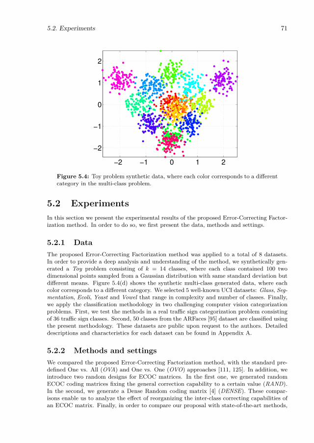
5.2. Experiments 71

−2 −1 0 1 2

−2

−1

0

1

2

Figure 5.4: Toy problem synthetic data, where each color corresponds to a differentcategory in the multi-class problem.

5.2 ExperimentsIn this section we present the experimental results of the proposed Error-Correcting Factor-ization method. In order to do so, we first present the data, methods and settings.

5.2.1 DataThe proposed Error-Correcting Factorization method was applied to a total of 8 datasets.In order to provide a deep analysis and understanding of the method, we synthetically gen-erated a Toy problem consisting of k = 14 classes, where each class contained 100 twodimensional points sampled from a Gaussian distribution with same standard deviation butdifferent means. Figure 5.4(d) shows the synthetic multi-class generated data, where eachcolor corresponds to a different category. We selected 5 well-known UCI datasets: Glass, Seg-mentation, Ecoli, Yeast and Vowel that range in complexity and number of classes. Finally,we apply the classification methodology in two challenging computer vision categorizationproblems. First, we test the methods in a real traffic sign categorization problem consistingof 36 traffic sign classes. Second, 50 classes from the ARFaces [95] dataset are classified usingthe present methodology. These datasets are public upon request to the authors. Detaileddescriptions and characteristics for each dataset can be found in Appendix A.

5.2.2 Methods and settingsWe compared the proposed Error-Correcting Factorization method, with the standard pre-defined One vs. All (OVA) and One vs. One (OVO) approaches [111, 125]. In addition, weintroduce two random designs for ECOC matrices. In the first one, we generated randomECOC coding matrices fixing the general correction capability to a certain value (RAND).In the second, we generate a Dense Random coding matrix [4] (DENSE). These compar-isons enable us to analyze the effect of reorganizing the inter-class correcting capabilities ofan ECOC matrix. Finally, in order to compare our proposal with state-of-the-art methods,

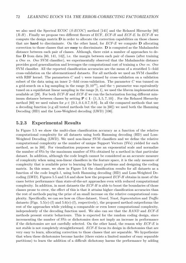
72 LEARNING ECOCS VIA THE ERROR-CORRECTING FACTORIZATION

we also used the Spectral ECOC (S-ECOC ) method [141] and the Relaxed Hierarchy [60](R-H ) . Finally we propose two different flavors of ECF, ECF-H and ECF-E. In ECF-H wecompute the design matrix D in order to allocate the correction capabilities on those classesthat are hard to discriminate. On the other hand, for ECF-E we compute D allocatingcorrection to those classes that are easy to discriminate. D is computed as the Mahalanobisdistance between each pair of classes. Although, there exist a number of approaches to de-fine D from data [60, 141, 142], i.e. the margin between each pair of classes (after traininga One vs. One SVM classifier), we experimentally observed that the Mahalanobis distanceprovides good generalization and leverages the computational cost of training a One vs. OneSVM classifier. All the reported classification accuracies are the mean of a stratified 5−foldcross-validation on the aforementioned datasets. For all methods we used an SVM classifierwith RBF kernel. The parameters C and γ were tunned by cross-validation on a validationsubset of the data using an inner 2−fold cross-validation. The parameter C was tunned ona grid-search on a log sampling in the range [0, 1010], and the γ parameter was equivalentlytuned on a equidistant linear sampling in the range [0, 1], we used the libsvm implementationavailable at [29]. For both ECF-H and ECF-E we run the factorization forcing different min-imum distance between classes by setting P ∈ 1 · 1, 3, 5, 7, 10 . For the Relaxed Hierarchymethod [60] we used values for ρ ∈ 0.1, 0.4, 0.7, 0.9. In all the compared methods that usea decoding function (e.g all tested methods but the one in [60]) we used both the HammingDecoding (HD) and the Loss-Weighted decoding (LWD) [106].

5.2.3 Experimental ResultsIn Figure 5.5 we show the multi-class classification accuracy as a function of the relativecomputational complexity for all datasets using both Hamming decoding (HD) and Loss-Weighted Decoding (LWD). We used non-linear SVM classifiers and we define the relativecomputational complexity as the number of unique Support Vectors (SVs) yielded for eachmethod, as in [60]. For visualization purposes we use an exponential scale and normalizethe number of SVs by the maximum number of SVs obtained by a method in that particulardataset. In addition, although the code length cannot be considered as an accurate measureof complexity when using non-linear classifiers in the feature space, it is the only measure ofcomplexity that is available prior to learning the binary problems and designing the codingmatrix. In this sense, we show in Figure 5.6 the classification results for all datasets as afunction of the code length l, using both Hamming decoding (HD) and Loss-Weighted De-coding (LWD). Figures 5.5 and 5.6 and show how the proposed ECF-H obtains in most of thecases better performance than state-of-the-art approaches even with reduced computationalcomplexity. In addition, in most datasets the ECF-H is able to boost the boundaries of thoseclasses prone to error, the effect of this is that it attains higher classification accuracies thanthe rest of methods paying the prize of an small increase on the relative computational com-plexity. Specifically, we can see how on Glass dataset, Vowel, Yeast, Segmentation and Trafficdatasets (Figs. 5.5(e)-(f) and 5.6(e)-(f), respectively), the proposed method outperforms therest of the approaches while yielding a comparable or even lower computational complexity,independently of the decoding function used. We also can see that the RAND and ECF-Emethods present erratic behaviours. This is expected for the random coding design, sinceincrementing the number of SVs or dichotomies does not imply an increase in performanceif the dichotomies are not carefully selected. On the other hand, the reason why ECF-E isnot stable is not completely straightforward. ECF-E focus its design in dichotomies that arevery easy to learn, allocating correction to those classes that are separable. We hypothesizethat when these dichotomies become harder (there exists a limited number of easy separablepartitions) to learn the addition of a difficult dichotomy harms the performance by adding

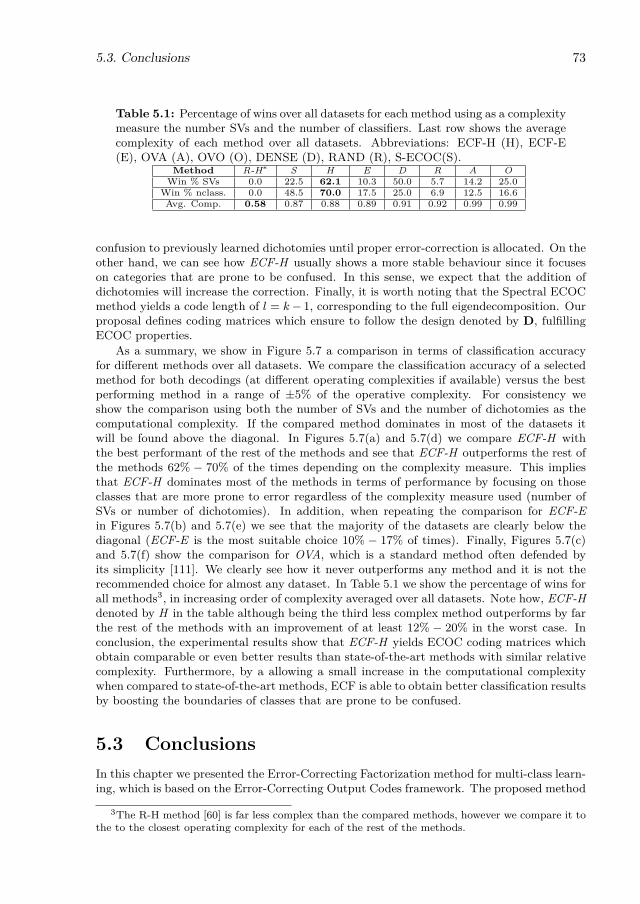
5.3. Conclusions 73

Table 5.1: Percentage of wins over all datasets for each method using as a complexitymeasure the number SVs and the number of classifiers. Last row shows the averagecomplexity of each method over all datasets. Abbreviations: ECF-H (H), ECF-E(E), OVA (A), OVO (O), DENSE (D), RAND (R), S-ECOC(S).

Method R-H∗ S H E D R A OWin % SVs 0.0 22.5 62.1 10.3 50.0 5.7 14.2 25.0

Win % nclass. 0.0 48.5 70.0 17.5 25.0 6.9 12.5 16.6Avg. Comp. 0.58 0.87 0.88 0.89 0.91 0.92 0.99 0.99

confusion to previously learned dichotomies until proper error-correction is allocated. On theother hand, we can see how ECF-H usually shows a more stable behaviour since it focuseson categories that are prone to be confused. In this sense, we expect that the addition ofdichotomies will increase the correction. Finally, it is worth noting that the Spectral ECOCmethod yields a code length of l = k− 1, corresponding to the full eigendecomposition. Ourproposal defines coding matrices which ensure to follow the design denoted by D, fulfillingECOC properties.

As a summary, we show in Figure 5.7 a comparison in terms of classification accuracyfor different methods over all datasets. We compare the classification accuracy of a selectedmethod for both decodings (at different operating complexities if available) versus the bestperforming method in a range of ±5% of the operative complexity. For consistency weshow the comparison using both the number of SVs and the number of dichotomies as thecomputational complexity. If the compared method dominates in most of the datasets itwill be found above the diagonal. In Figures 5.7(a) and 5.7(d) we compare ECF-H withthe best performant of the rest of the methods and see that ECF-H outperforms the rest ofthe methods 62% − 70% of the times depending on the complexity measure. This impliesthat ECF-H dominates most of the methods in terms of performance by focusing on thoseclasses that are more prone to error regardless of the complexity measure used (number ofSVs or number of dichotomies). In addition, when repeating the comparison for ECF-Ein Figures 5.7(b) and 5.7(e) we see that the majority of the datasets are clearly below thediagonal (ECF-E is the most suitable choice 10% − 17% of times). Finally, Figures 5.7(c)and 5.7(f) show the comparison for OVA, which is a standard method often defended byits simplicity [111]. We clearly see how it never outperforms any method and it is not therecommended choice for almost any dataset. In Table 5.1 we show the percentage of wins forall methods3, in increasing order of complexity averaged over all datasets. Note how, ECF-Hdenoted by H in the table although being the third less complex method outperforms by farthe rest of the methods with an improvement of at least 12% − 20% in the worst case. Inconclusion, the experimental results show that ECF-H yields ECOC coding matrices whichobtain comparable or even better results than state-of-the-art methods with similar relativecomplexity. Furthermore, by a allowing a small increase in the computational complexitywhen compared to state-of-the-art methods, ECF is able to obtain better classification resultsby boosting the boundaries of classes that are prone to be confused.

5.3 ConclusionsIn this chapter we presented the Error-Correcting Factorization method for multi-class learn-ing, which is based on the Error-Correcting Output Codes framework. The proposed method

3The R-H method [60] is far less complex than the compared methods, however we compare it tothe to the closest operating complexity for each of the rest of the methods.

74 LEARNING ECOCS VIA THE ERROR-CORRECTING FACTORIZATION

0.19 0.85 0.92 0.96 0.99

0.5

0.6

0.7

0.8

0.19 0.85 0.92 0.96 0.990.6

0.7

0.8

0.37 0.85 0.92 0.96 0.990.3

0.4

0.5

0.6

0.7

0.8

0.37 0.85 0.92 0.96 0.990.4

0.5

0.6

0.7

0.8

(a)Toy dataset HD (b)Toy dataset LWD (c)Ecoli dataset HD (d) Ecoli dataset LWD

0.58 0.85 0.92 0.96 0.99

0.4

0.5

0.6

0.58 0.85 0.92 0.96 0.99

0.5

0.6

0.51 0.85 0.92 0.96 0.990.6

0.7

0.8

0.9

1

0.51 0.85 0.92 0.96 0.990.6

0.7

0.8

0.9

1

(e)Glass dataset HD (f)Glass dataset LWD (j)Vowel dataset HD (h) Vowel dataset LWD

0.75 0.85 0.92 0.96 0.99

0.4

0.5

0.6

0.75 0.85 0.92 0.96 0.99

0.4

0.5

0.6

0.3 0.6 0.8 10.8

0.9

0.3 0.6 0.8 10.8

0.9

(i)Yeast dataset HD (j)Yeast dataset LWD (k)Segment. dataset HD(l) Segment. dataset LWD

0.85 0.92 0.96 0.99

0.2

0.4

0.6

0.8

0.85 0.92 0.96 0.99

0.2

0.4

0.6

0.8

0.85 0.92 0.96 0.990.20.30.40.50.60.70.80.9

0.61 0.85 0.92 0.96 0.990.20.30.40.50.60.70.80.9

(e)Traffic dataset HD (f)Traffic dataset LWD (j)ARFace dataset HD (h)ARFace dataset LWD

ECF-H ECF-E S-ECOC R-H RAND DENSE OVO OVA

Figure 5.5: Multi-class classification accuracy (y axis) as a function of the relativecomputational complexity (x axis) for all datasets and both decoding measures.

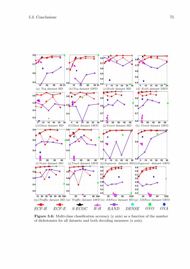
5.3. Conclusions 75

10 20 30 40 91

0.5

0.6

0.7

0.8

10 20 30 40 91

0.6

0.7

5 10 15 20 25 300.3

0.4

0.5

0.6

0.7

0.8

5 10 15 20 25 30

0.4

0.5

0.6

0.7

0.8

(a) Toy dataset HD (b)Toy dataset LWD (c)Ecoli dataset HD (d) Ecoli dataset LWD

5 10 15 20 25 30

0.3

0.4

0.5

0.6

5 10 15 20 25 30

0.4

0.5

0.6

10 20 30 40 500.6

0.7

0.8

0.9

10 20 30 40 500.6

0.7

0.8

0.9

(e)Glass dataset HD (f)Glass dataset LWD (j)Vowel dataset HD (h) Vowel dataset LWD

10 20 30 40

0.4

0.5

0.6

10 20 30 40

0.4

0.5

0.6

5 10 15 20 25 300.8

0.9

5 10 15 20 25 300.8

0.9

(i)Yeast dataset HD (j)Yeast dataset LWD (k)Segment. dataset HD(l)Segment. dataset LWD

10 20 30 40 50 60 630

0.2

0.4

0.6

0.8

20 40 60 630

0.2

0.4

0.6

0.8

20 40 60 1225

0.2

0.3

0.4

0.5

0.6

0.7

0.8

0.9

20 40 60 1225

0.2

0.3

0.4

0.5

0.6

0.7

0.8

0.9

(m)Traffic dataset HD (n) Traffic dataset LWD(o) ARFace dataset HD(p) ARFace dataset LWD

ECF-H ECF-E S-ECOC R-H RAND DENSE OVO OVA

Figure 5.6: Multi-class classification accuracy (y axis) as a function of the numberof dichotomies for all datasets and both decoding measures (x axis).

76 LEARNING ECOCS VIA THE ERROR-CORRECTING FACTORIZATION

0.4 0.6 0.8 10.4

0.5

0.6

0.7

0.8

0.9

1

EC

F−

H c

las

sif

icati

on

ac

cu

rac

y

best classification accuracy0.4 0.6 0.8 1

0.4

0.5

0.6

0.7

0.8

0.9

1

EC

F−

E c

las

sif

ica

tio

n a

cc

ura

cy

best classification accuracy0.2 0.4 0.6 0.8 1

0.2

0.3

0.4

0.5

0.6

0.7

0.8

0.9

1

OV

A c

las

sif

ica

tio

n a

cc

ura

cy

best classification accuracy

(a) (b) (c)

0.4 0.6 0.8 10.4

0.5

0.6

0.7

0.8

0.9

1

EC

F−

H c

las

sif

ica

tio

n a

cc

ura

cy

best classification accuracy0.4 0.6 0.8 1

0.4

0.5

0.6

0.7

0.8

0.9

1

EC

F−

E c

las

sif

ica

tio

n a

cc

ura

cy

best classification accuracy0.2 0.4 0.6 0.8 1

0.2

0.3

0.4

0.5

0.6

0.7

0.8

0.9

1

OV

A c

las

sif

ica

tio

n a

cc

ura

cy

best classification accuracy

(d) (e) (f)

Figure 5.7: (a) Summary of performance of ECF-H method over all datasets usingthe number of SVs and the number of dichotomies as the measure of complexity,respectively for ECF-H (a)(d), ECF-E (b)(e) and OVA (c)(f).

factorizes a design matrix of desired correction properties into a discrete Error-Correctingcomponent consistent with the design matrix. ECF is a general method for building anECOC multi-class classifier with desired properties, which can be either directly set by theuser or obtained from data using a priori inter-class distances. We note that the proposedapproach is not a replacement for ECOC codings, but a generalized framework to buildECOC matrices that follow a certain error-correcting criterion design. The Error-CorrectingFactorization is formulated as a minimization problem which is optimized using a constrainedCoordinate Descent, where the minimizer of each coordinate is the solution to a least-squaresproblem with box and linear constraints that can be efficiently solved. By analyzing the ap-proximation error, we empirically show that although ECF is a non-convex optimizationproblem, the optimization is very efficient. We performed experiments using ECF to buildECOC matrices following the common trend in state-of-the-art works, in which the designmatrix priorized the most separable classes. In addition, we hypothesized and showed thata more beneficial situation is to allocate the correction capability of the ECOC to thosecategories which are more prone to confusion. Experiments show that when ECF is used toallocate the correction capabilities to those classes which are prone to confusion we obtainhigher accuracies than state of the art methods with efficient models in terms of the numberof Support Vectors and dichotomies.

Finally, there still exists open questions that require a deeper analysis for future work.The results obtained raise a fair doubt regarding the right allocation of error correcting

5.3. Conclusions 77

power in several methods found in literature where ECOC designs are based on the premiseof boosting the classes which are easily separable. In the light of these results, we mayconjecture that a careful allocation of error correction must be made in such a way thatbalances two aspects: on one hand, simple to classify boundaries must be handled properly.On the other hand, the error correction must be allocated on difficult classes for the ensembleto correct possible mistakes. In addition, it would be interesting to study which are theparameters that affect the suitability of the no class is left behind and the hard classes areleft behind one. Finally we could consider ternary matrices and further regularizations.

78 LEARNING ECOCS VIA THE ERROR-CORRECTING FACTORIZATION

Part III

Applications in PoseEstimation Problems

79

Chapter 6

Applications of ECOCs in PoseEstimation Problems

The problem of recovering the pose of human beings in images has always attracted a lot ofattention, due to the huge amount of possible applications in fields like Human-ComputerInteraction, Surveillance, eHealth, or Gaming. Nevertheless, human multi-limb segmentationis a very hard task because of dramatic potential changes in appearance produced by differentpoints of view, clothing, lighting conditions, occlusions, and number of articulations of thehuman body. From the perspective of Machine Learning the task of estimating the poseof the human body in images is often modeled as a multi-class classification problem, inwhich for each pixel in the image a label denoting a human limb (or background) has to beestimated. Hence, rendering this problem suitable for the Error-Correcting Output Codesframework.

In this chapter we present our contributions in human pose estimation by using ECOCs.In particular we propose a two-stage approach for the segmentation of human limbs, basedon the ECOC framework and Graph-Cuts optimization. Furthermore, we also introducethe HuPBA 8k+ dataset, which is one the biggest datasets in for human pose estimation inliterature. The dataset contains more than 8000 labeled frames at pixel precision, includingmore than 120000 manually labeled samples of 14 different limbs.

6.1 Human Pose EstimationThe common pipeline for human pose estimation in visual data is usually defined in a bottom-up fashion. First, the human body limbs are segmented and the body pose is estimated(often with a prior person/background segmentation or person detection step). Then, oncethe body pose is estimated higher abstraction analysis can be performed using the predictedskeletal model.

The first step of the pipeline, which concerns pose estimation in RGB images has beena core problem in the Computer Vision field since its early beginnings. In this particularproblem the goal is to provide a label for each pixel in the image whether it belongs to acertain body limb or to the background class, discriminating human limbs from each otherand from the rest of the image. Usually, human body segmentation is treated in a two-stagefashion. First, a human body part detection step is performed, and then, these human partdetections are used as a prior knowledge to be optimized by segmentation/inference strategies

81

82 APPLICATIONS OF ECOCS IN POSE ESTIMATION PROBLEMS

in order to encode the natural relations of the different limbs and obtain the final human-limb semantic segmentation. In literature one can find many works that follow this two-stagescheme. Bourdev et. al. [19] used body part detections in an AND-OR graph to obtain thepose estimation. Vinet et. al [130] proposed to use Conditional Random Fields based onbody part detectors to obtain a complete person/background segmentation. Nevertheless,one of the methods that have generated more attraction is the well known pictorial structurefor object recognition introduced by Felzenszwalb et al [54]. Some works have applied anadaptation of pictorial structures using a set of joint limb marks to infer spatial probabilities[6, 108, 109, 118]. Later on, an extension was presented by Yang and Ramanan [138, 139]which proposed a discriminatively trained pictorial structure that models the body jointsinstead of limbs. In contrast, there is also current tendency to use Graph Cuts optimizationto segment the human limbs [68] or full person segmentation [114].

The Computer Vision community has been lately focusing their efforts on developingmethods for both pose estimation and action/gesture recognition. However, one of themain problems is the necessity of public available data sets containing annotations of all thevariabilities the methods have to deal with. Substantial effort has been put on designingdatasets with different scenarios, people and illumination characteristics. Datasets such asParse [108], Buffy [55], UIUC People [126], and Pascal VOC [53] are widely used to evaluatedifferent pose estimation and action/gesture recognition methods. However, these publicavailable datasets fail to provide with a sound framework in which to validate pose recoverysystems (i.e. the number of samples per limb is small, the labeling is not accurate, there areno interactions of actors, etc.). Given this lack of sound and refined public datasets for humanmulti-limb segmentation and/or action/gesture recognition, in this thesis we introduce theHuPBA 8k+ dataset, which to the best of our knowledge is the biggest RGB human-limblabeled dataset. The dataset contains more than 8000 labeled frames at pixel precision andmore than 120000 manually labeled samples of 14 different limbs.

Furthermore, in this chapter of the thesis we also propose a two-stage approach for thesegmentation of human limbs. In a first stage, a set of human limbs are normalized bymain orientation to be rotation invariant, described using Haar-like features, and trainedusing cascades of Adaboost classifiers to be split in a tree-structure way. Once the tree-structure is trained, it is included in a ternary ECOC framework. This first classificationstep is applied in a windowing way on a new test image, defining a body-like probabilitymap, which is used as an initialization of a binary Graph Cuts optimization procedure.In the second stage, we embed a similar tree-structured partition of limbs in a ternaryECOC framework and we use Support Vector Machines (SVMs) with HOG descriptors tobuild a more accurate set of limb-like probability maps within the segmented user binarymask, that are fed to a multi-label GraphCut optimization procedure to obtain the finalhuman multi-limb segmentation. We tested our ECOC-Graph-Cut based approach in thenovel HuPBA 8k+ dataset and compared with state-of-the-art pose recovery approaches,obtaining performance improvements. Summarizing, our key contributions for this chapterare:

• We introduce the HuPBA 8k+ dataset, the largest RGB labeled dataset of humanlimbs, with more than 120000 manually annotated limbs.

• We propose a two stage approach based on ECOC and Graph Cuts for the segmenta-tion of human limbs in RGB images.

• The proposed method is compared with state-of-the-art methods for human pose es-timation obtaining very satisfying results.

6.2. HuPBA 8K+ Dataset 83

6.2 HuPBA 8K+ DatasetHuman pose recovery is a challenging problem in Computer Vision, not only for the intrinsiccomplexity of the task, but also for the lack of large public and annotated datasets. Usually,public available datasets lack of refined labeling or contain a very reduced number of samplesper limb (e.g. Buffy Stickmen V3.01, Leeds Sports and Hollywood Human Actions [55, 77,85]). In addition, large datasets often use synthetic samples or capture human limbs withsensor technologies such as MoCap in very controlled environments [37].

Being aware of this lack of public available datasets for multi-limb human pose detection,segmentation and action/gesture recognition, we present a novel fully limb labeled dataset,the HuPBA 8k+ dataset. This dataset is formed by more than 8000 frames where 14 limbsare labeled at pixel precision1.

1. The images are obtained from 9 videos (RGB sequences) and a total of 14 differentactors appear in those 9 sequences. In concrete, each sequence has a main actor (9in total) which during the video interacts with secondary actors performing a set ofdifferent actions.

2. RGB images were stored with resolution 480× 360 in BMP file format.

3. For each actor present in an image 14 limbs (if not occluded) were manually tagged:Head, Torso, R-L Upper-arm, R-L Lower-arm, R-L Hand, R-L Upper-leg, R-L Lower-leg, and R-L Foot.

4. Limbs are manually labeled using binary masks and the minimum bounding box con-taining each subject is defined.

5. The actors appear in a wide range of different poses.

Sample of different poses in the HuPBA 8k+ dataset are show in Figure 6.1. Furtherdetails of the dataset can be found in [117].

Finally, in Table 6.1 we compare the HuPBA 8k+ dataset characteristics with some pub-licly available datasets. These public datasets are chosen taking into account the variabilityof limbs and gestures/actions. Once can see that the novel dataset offers higher numberof annotated limbs at pixel precision in comparison with state-of-the-art public availabledatasets.

HuPBAPARSE[108]BUFFY[55]UIUC[126]LEEDS[77]HW[85]MMGR13[46]H.Actions[120]Pascal VOC[53]Labeling at

pixelprecision

Yes No No No No - No No Yes

Number oflimbs 14 10 6 14 14 - 16 - 5

Number oflabeled limbs124 761 3 050 4 488 18 186 28 000 - 27 532 800 - 8 500

Number offrames 8 234 305 748 1 299 2 000 - 1 720 800 - 1 218

Full body Yes Yes No Yes Yes - Yes Yes YesLimb

annotation Yes Yes Yes Yes Yes No Yes No Yes

Gestureannotation Yes No No No No Yes Yes Yes No

Number ofgestures 11 - - - - 8 20 6 -

Number ofgesturesamples

235 - - - - 430 13 858 600 -

Table 6.1: Comparison of public dataset characteristics.

1The whole number of manual labeled limbs exceeds 120000.

84 APPLICATIONS OF ECOCS IN POSE ESTIMATION PROBLEMS

6.3 ECOC and GraphCut based multi-limb segmen-tation

In the following subsections we describe the proposed ECOC-based method for automaticsegmentation of human limbs. To accomplish this task, we define a framework divided intwo stages. The first stage, focused on binary person/background segmentation, is split infour main steps: a) Body part learning using cascade of classifiers, b) Tree-structure learningof human limbs, c) ECOC multi-limb detection, and d) Binary GrabCut optimization forforeground extraction. In the second stage, we segment the person/background binary maskinto different limb regions. This stage is split in the following four steps: e) Tree-structurebody part learning without background, f) ECOC multi-limb detection, g) Limb-like prob-ability map definition, and h) Alpha-beta swap Graph Cuts multi-limb segmentation. Thescheme of the proposed system is illustrated in Fig. 6.2.

6.3.1 Body part learning using cascade of classifiersThe core of most human body segmentation methods in the literature relies on body partdetectors. In this sense, most part detectors in literature follow a cascade of classifiersarchitecture [30, 43, 57, 97, 148]. Cascades of classifiers are based on the idea of learningand unbalanced binary problem by using the negative outputs of a classifier f i as an inputfor the following classifier f i+1. Particularly, this cascade structure allows any classifier torefine the prediction by reducing the false positive rate at every stage of the cascade. Inthis sense, we use AdaBoost as the base classifier in our cascade architecture. In addition,in order to make the body part detection rotation invariant, all body parts are rotated tothe dominant gradient region orientation. Then, Haar-like features are used to describe thebody parts.

Because of its properties, cascade of classifiers are usually trained to split one visual objectfrom the rest of possible objects of an image. This means that the cascade of classifiers learnsto detect a certain object (body part in our case), ignoring all other objects (all other bodyparts). However, if we define our problem as a multi-limb detection procedure, some bodyparts are similar in appearance, and thus, it makes sense to group them in the same visualcategory. Because of this reason, we propose to learn a set of cascade of classifiers where asubset of limbs are included in the positive set of a cascade, and the remaining limbs areincluded as negative instances together with background images in the negative set of thecascade. Applying this grouping for different cascades of classifiers in a tree-structure wayand combining them in an Error-Correcting Output Codes (ECOC) framework enables thesystem to perform multi-limb detection [50].

6.3.2 Tree-structure learning of human limbsThe first issue to take into account when defining a set of cascades of classifiers is how todefine the groups of limbs to be learnt by each individual cascade. For this task, we proposeto train a tree-structure cascade of classifiers. This tree-structure defines the set of meta-classes for each dichotomy (cascade of classifiers) taking into account the visual appearanceof body parts, which has two purposes. On one hand, we aim to avoid dichotomies in whichbody parts with different visual appearance belong to the same meta-class. On the otherhand, the dichotomies that deal with classes that are difficult to learn (body parts withsimilar visual appearance) are defined taking into account few classes. An example of thebody part tree-structure defined taking into account these issues for a set of 7 body limbs isshown in Fig. 6.3(a). Notice that classes with similar visual appearance (e.g. upper-arm and

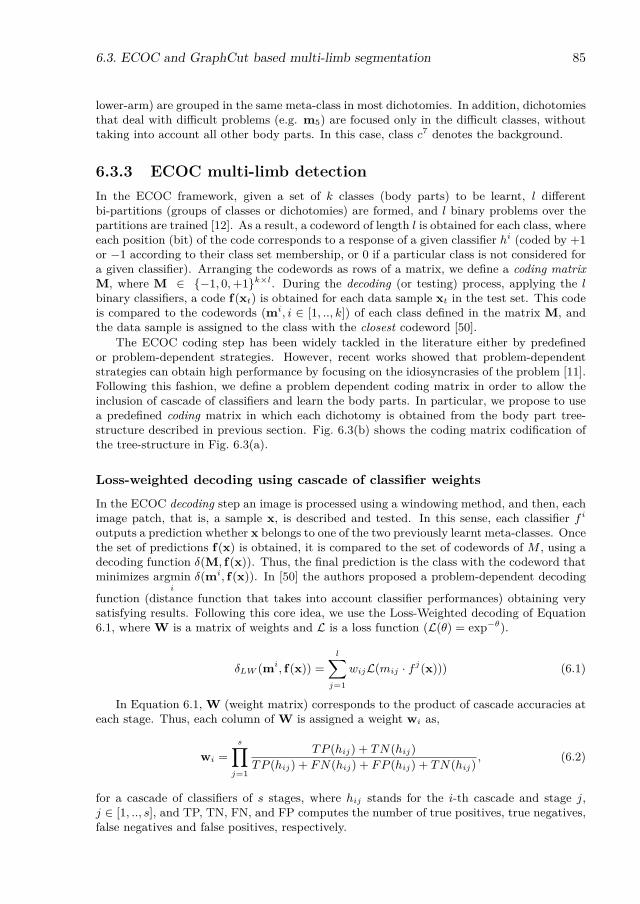
6.3. ECOC and GraphCut based multi-limb segmentation 85

lower-arm) are grouped in the same meta-class in most dichotomies. In addition, dichotomiesthat deal with difficult problems (e.g. m5) are focused only in the difficult classes, withouttaking into account all other body parts. In this case, class c7 denotes the background.

6.3.3 ECOC multi-limb detectionIn the ECOC framework, given a set of k classes (body parts) to be learnt, l differentbi-partitions (groups of classes or dichotomies) are formed, and l binary problems over thepartitions are trained [12]. As a result, a codeword of length l is obtained for each class, whereeach position (bit) of the code corresponds to a response of a given classifier hi (coded by +1or −1 according to their class set membership, or 0 if a particular class is not considered fora given classifier). Arranging the codewords as rows of a matrix, we define a coding matrixM, where M ∈ −1, 0,+1k×l. During the decoding (or testing) process, applying the lbinary classifiers, a code f(xt) is obtained for each data sample xt in the test set. This codeis compared to the codewords (mi, i ∈ [1, .., k]) of each class defined in the matrix M, andthe data sample is assigned to the class with the closest codeword [50].

The ECOC coding step has been widely tackled in the literature either by predefinedor problem-dependent strategies. However, recent works showed that problem-dependentstrategies can obtain high performance by focusing on the idiosyncrasies of the problem [11].Following this fashion, we define a problem dependent coding matrix in order to allow theinclusion of cascade of classifiers and learn the body parts. In particular, we propose to usea predefined coding matrix in which each dichotomy is obtained from the body part tree-structure described in previous section. Fig. 6.3(b) shows the coding matrix codification ofthe tree-structure in Fig. 6.3(a).

Loss-weighted decoding using cascade of classifier weights

In the ECOC decoding step an image is processed using a windowing method, and then, eachimage patch, that is, a sample x, is described and tested. In this sense, each classifier f ioutputs a prediction whether x belongs to one of the two previously learnt meta-classes. Oncethe set of predictions f(x) is obtained, it is compared to the set of codewords of M , using adecoding function δ(M, f(x)). Thus, the final prediction is the class with the codeword thatminimizes argmin

i

δ(mi, f(x)). In [50] the authors proposed a problem-dependent decoding

function (distance function that takes into account classifier performances) obtaining verysatisfying results. Following this core idea, we use the Loss-Weighted decoding of Equation6.1, where W is a matrix of weights and L is a loss function (L(θ) = exp−θ).

δLW (mi, f(x)) =l∑

j=1

wijL(mij · f j(x))) (6.1)

In Equation 6.1, W (weight matrix) corresponds to the product of cascade accuracies ateach stage. Thus, each column of W is assigned a weight wi as,

wi =s∏j=1

TP (hij) + TN(hij)TP (hij) + FN(hij) + FP (hij) + TN(hij)

, (6.2)

for a cascade of classifiers of s stages, where hij stands for the i-th cascade and stage j,j ∈ [1, .., s], and TP, TN, FN, and FP computes the number of true positives, true negatives,false negatives and false positives, respectively.

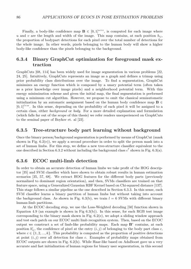
86 APPLICATIONS OF ECOCS IN POSE ESTIMATION PROBLEMS

Finally, a body-like confidence map B ∈ [0, 1]u×v, is computed for each image whereu and v are the length and width of the image. This map contains, at each position bij ,the proportion of bodypart detections for each pixel over the total number of detections forthe whole image. In other words, pixels belonging to the human body will show a higherbody-like confidence than the pixels belonging to the background.

6.3.4 Binary GraphCut optimization for foreground mask ex-traction

GraphCuts [68, 114] has been widely used for image segmentation in various problems [22,24, 25]. Intuitively, GraphCuts represents an image as a graph and defines a trimap usingprior probability class distributions over the image. To find a segmentation, GraphCutminimizes an energy function which is composed by a unary potential term (often takenas a prior knowledge over image pixels) and a neighborhood potential term. With thisenergy minimization scheme and given the initial map, the final segmentation is performedusing a minimum cut algorithm. However, we propose to omit the classical semiautomaticinitialization by an automatic assignment based on the human body confidence map B ∈[0, 1]l×w. In this sense, depending on the probability of each pixel it will be assigned to acertain class, either background or body. For a more detailed explanation and formulation(which falls far out of the scope of this thesis) we refer readers unexperienced on GraphCutsto the seminal paper of Boykov et. al [23].

6.3.5 Tree-structure body part learning without backgroundOnce the binary person/background segmentation is performed by means of GraphCut (maskshown in Fig. 6.2(e)), we apply a second procedure in order to split the person mask into aset of human limbs. For this step, we define a new tree-structure classifier equivalent to theone described in Section 6.3.2 without including the background class c7 shown in Fig. 6.3(a).

6.3.6 ECOC multi-limb detectionIn order to obtain an accurate detection of human limbs we take profit of the HOG descrip-tor [35] and SVM classifier which have shown to obtain robust results in human estimationscenarios [35, 57, 68]. We extract HOG features for the different body parts (previouslynormalized to dominant region orientation), and then, SVMs classifiers are trained on thatfeature space, using a Generalized Gaussian RBF Kernel based on Chi-squared distance [137].This stage follows a similar pipeline as the one described in Section 6.3.3. In this sense, eachSVM classifier learns a binary partition of human limbs but without taking into accountthe background class. As shown in Fig. 6.3(b), we train l = 6 SVMs with different binaryhuman-limb partitions.

At the ECOC decoding step, we use the Loss-Weighted decoding [50] function shown inEquation 4.9 (an example is shown in Fig 6.3(b)). In this sense, for each RGB test imagecorresponding to the binary mask shown in Fig. 6.2(e), we adopt a sliding window approachand test each patch on our ECOC multi limb recognition system. Then, based on the ECOCoutput we construct a set of limb-like probability maps. Each map Bc contains, at eachposition bcij , the confidence of pixel at the entry (i, j) of belonging to the body part class c,where c ∈ 1, 2, ..., k. This probability is computed as the proportion of positive detectionsat point (i, j) over all detection for class c. Examples of probability maps obtained fromECOC outputs are shown in Fig. 6.2(h). While Haar-like based on AdaBoost gave us a veryaccurate and fast initialization of human regions for binary user segmentation, in this second

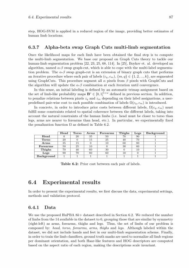
6.4. Experimental results 87

step, HOG-SVM is applied in a reduced region of the image, providing better estimates ofhuman limb locations.

6.3.7 Alpha-beta swap Graph Cuts multi-limb segmentationOnce the likelihood maps for each limb have been obtained the final step is to computethe multi-limb segmentation. We base our proposal on Graph Cuts theory to tackle ourhuman-limb segmentation problem [22, 23, 25, 68, 114]. In [25], Boykov et. al. developed analgorithm, named α-β swap graph-cut, which is able to cope with the multi-label segmenta-tion problem. The α-β swap graph-cut is an extension of binary graph cuts that performsan iterative procedure where each pair of labels (cq, cm), m, q ∈ 1, 2, ..., k, are segmentedusing GraphCuts. This procedure segment all α pixels from β pixels with GraphCuts andthe algorithm will update the α-β combination at each iteration until convergence.

In this sense, an initial labeling is defined by an automatic trimap assignment based onthe set of limb-like probability maps Bc ∈ [0, 1]l×w defined in previous section. In addition,to penalize relations between pixels zq and zm depending on their label assignations, a user-predefined pair-wise cost to each possible combination of labels Ω(cq, cm) is introduced.

In concrete, in order to introduce prior costs between different labels, Ω(cq, cm) mustfulfill some constraints related to spatial coherence between the different labels, taking intoaccount the natural constraints of the human limbs (i.e. head must be closer to torso thanlegs, arms are nearer to forearms than head, etc.). In particular, we experimentally fixedthe penalization function Ω as defined in Table 6.2.

Head Torso Arms Forearms Thighs Legs BackgroundHead 0 20 35 50 70 90 1Torso 20 0 15 25 40 70 1Arms 35 15 0 10 60 80 1

Forearms 50 25 10 0 30 60 1Thighs 70 40 60 30 0 10 1Legs 90 70 80 60 10 0 1

Background 1 1 1 1 1 1 1

Table 6.2: Prior cost between each pair of labels.

6.4 Experimental resultsIn order to present the experimental results, we first discuss the data, experimental settings,methods and validation protocol.

6.4.1 DataWe use the proposed HuPBA 8k+ dataset described in Section 6.2. We reduced the numberof limbs from the 14 available in the dataset to 6, grouping those that are similar by symmetry(right-left) as arms, forearms, thighs and legs. Thus, the set of limbs of our problem iscomposed by: head, torso, forearms, arms, thighs and legs. Although labeled within thedataset, we did not include hands and feet in our multi-limb segmentation scheme. Finally,in order to train the limb classifiers, ground truth masks are used to normalize all limb regionsper dominant orientation, and both Haar-like features and HOG descriptors are computedbased on the aspect ratio of each region, making the descriptions scale invariant.

88 APPLICATIONS OF ECOCS IN POSE ESTIMATION PROBLEMS

6.4.2 Methods and experimental settingsTo evaluate the performance of our proposal for multi-limb segmentation, we compare ourstrategy with two state-of-the-art methods for multi-limb segmentation:

• FMP: This method was proposed by Yang and Ramanan [138, 139] and it is based onFlexible Mixtures-of-Parts (FMP). We compute the average of each set of mixtures foreach limb and for each pyramid level in order to obtain the probability maps for eachlimb category. In order to compute the probability map of the background category,we subtract 1 with the maximum probability ∈ [0, 1] of the set of limbs detection atpixel location.

• IPP: This method is proposed by Ramanan [108] and it is based on an IterativeParsing Process (IPP). We use it to extract the limb-like probability maps followed byα-β swap graph-cut multi-limb segmentation. The background category is computedas described for the FMP method.

• ECOC+GraphCut: Our proposed human limb segmentation scheme shown in Fig. 6.2.

Experimental settingsIn a preprocessing step, we resized all limb samples to a 32×32 pixels region for computationalpurposes. Then, we used the standard Cascade of Classifiers based on AdaBoost and Haar-like features [131], and we forced a 0.99 false positive rate and maximum of 0.4 false alarmrate during 8 stages. To detect limbs with trained cascades of classifiers, we applied a slidingwindow approach with an initial patch size of 32× 32 pixels up to 60× 60 pixels. As a finalpart of the first stage, binary Graph Cuts were applied to obtain the binary segmentationwhere the initialization values of foreground and background were provided to the binaryGraph Cut algorithm and tuned via cross-validation.

For the second stage, we set the following parameters for the HOG descriptor: 32 × 32window size, 16×16 block size, 8×8 block stride, 8×8 cell size and 8 for number of bins. Then,we trained SVMs with a Generalized Gaussian RBF kernel based on Chi-squared distance,(see Fig.(a) 6.3). The parameters of the kernel, C and γ were tuned via cross-validation.Finally, the model selection step was done via a leave-one-sequence-out cross-validation. Formulti-limb segmentation we used the alpha-beta GraphCut procedure, where we set a 8× 8neighboring grid and tuned the λ parameter of GraphCut using cross-validation.

6.4.3 Validation measurementIn order to evaluate the results for the two different tasks: binary segmentation and multi-

label segmentation, we use the Jaccard Index of overlapping (J =A⋂B

A⋃B) where A is the

ground-truth and B is the corresponding prediction.

6.4.4 Multi-limb segmentation resultsFor the Multi-limb segmentation task, we show in Fig. 6.4 and Fig. 6.5 qualitative resultsfor some samples of the HuPBA 8k+ dataset. When comparing the qualitative results wecan see how the FMP method [138, 139] performs worse than its counter parts. In addition,one can se how IPP and our method obtain similar results in most cases. However, the IPPlacks of a good person/background segmentation.

Furthermore, we provide with quantitative results in terms of the Jaccard Index. InFig. 6.6 we show the overlapping performance obtained by the different methods, where each

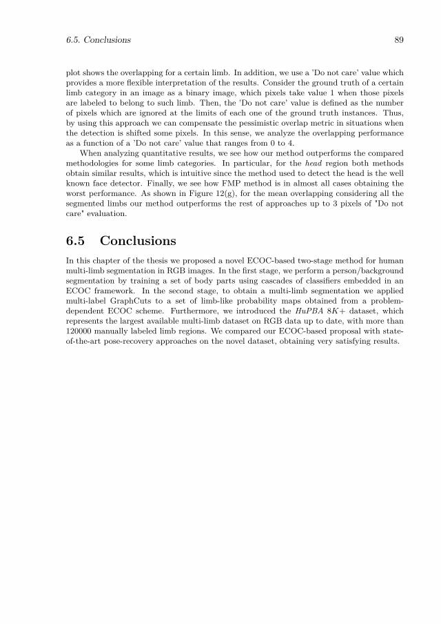
6.5. Conclusions 89

plot shows the overlapping for a certain limb. In addition, we use a ’Do not care’ value whichprovides a more flexible interpretation of the results. Consider the ground truth of a certainlimb category in an image as a binary image, which pixels take value 1 when those pixelsare labeled to belong to such limb. Then, the ’Do not care’ value is defined as the numberof pixels which are ignored at the limits of each one of the ground truth instances. Thus,by using this approach we can compensate the pessimistic overlap metric in situations whenthe detection is shifted some pixels. In this sense, we analyze the overlapping performanceas a function of a ’Do not care’ value that ranges from 0 to 4.

When analyzing quantitative results, we see how our method outperforms the comparedmethodologies for some limb categories. In particular, for the head region both methodsobtain similar results, which is intuitive since the method used to detect the head is the wellknown face detector. Finally, we see how FMP method is in almost all cases obtaining theworst performance. As shown in Figure 12(g), for the mean overlapping considering all thesegmented limbs our method outperforms the rest of approaches up to 3 pixels of "Do notcare" evaluation.

6.5 ConclusionsIn this chapter of the thesis we proposed a novel ECOC-based two-stage method for humanmulti-limb segmentation in RGB images. In the first stage, we perform a person/backgroundsegmentation by training a set of body parts using cascades of classifiers embedded in anECOC framework. In the second stage, to obtain a multi-limb segmentation we appliedmulti-label GraphCuts to a set of limb-like probability maps obtained from a problem-dependent ECOC scheme. Furthermore, we introduced the HuPBA 8K+ dataset, whichrepresents the largest available multi-limb dataset on RGB data up to date, with more than120000 manually labeled limb regions. We compared our ECOC-based proposal with state-of-the-art pose-recovery approaches on the novel dataset, obtaining very satisfying results.

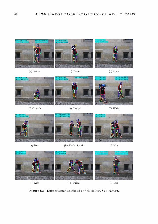
90 APPLICATIONS OF ECOCS IN POSE ESTIMATION PROBLEMS

(a) Wave (b) Point (c) Clap

(d) Crouch (e) Jump (f) Walk

(g) Run (h) Shake hands (i) Hug

(j) Kiss (k) Fight (l) Idle

Figure 6.1: Different samples labeled on the HuPBA 8k+ dataset.

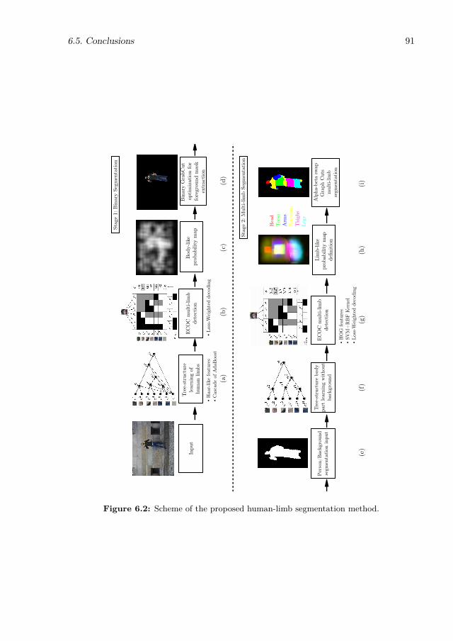
6.5. Conclusions 91

E

CO

C m

ulti

­lim

bde

tect

ion

Bin

ary

Gra

bCut

op

tim

izat

ion

for

fore

grou

nd m

ask

extr

acti

on

Stag

e 1:

Bin

ary

Segm

enta

tion

Stag

e 2:

Mul

ti­li

mb

Segm

enta

tion

Tre

e­st

ruct

ure

body

part

lear

ning

witho

utba

ckgr

ound

A

lpha

­bet

a sw

apG

raph

Cut

s m

ulti­li

mb

segm

enta

tion

H

aar­

like

feat

ures

C

asca

de o

f A

daB

oost

L

oss­

Wei

ghte

d de

codi

ng

H

OG

fea

ture

s S

VM

+R

BF K

erne

l L

oss­

Wei

ghte

d de

codi

ng

EC

OC

mul

ti­li

mb

dete

ctio

n

(a)

(b)

(c)

(d)

Bod

y­lik

e pr

obab

ility

map

Lim

b­lik

epr

obab

ility

map

de

finitio

n

(e)

(f)

(g)

(h)

Per

son/

Bac

kgro

und

segm

enta

tion

inpu

t

Tre

e­st

ruct

ure

lear

ning

of

hum

an li

mbs

Inpu

t

(i)

Hea

dTor

so

Arm

sFo

rear

ms

Thi

ghs

Legs

Figure 6.2: Scheme of the proposed human-limb segmentation method.

92 APPLICATIONS OF ECOCS IN POSE ESTIMATION PROBLEMS

δδ

h(x)

0.91

0.83

0.99

0.63

0.89

0.270.45

m1

m2

m3

m4

m5

m6

c1

c2

c3

c4

c5

c6

c7

(a) (b)

w1 w2 w3 w4 w5 w6

Head

Torso

Arm

Forearm

Thigh

Leg

Background

m1 m3

m1

m2

m2

m3

m4

m5

m6

m7

m4m5 m6

Figure 6.3: (a) Tree-structure classifier of body parts, where nodes represent the defineddichotomies. Notice that the single or double lines indicate the meta-class defined. (b) ECOCdecoding step, in which a head sample is classified. The coding matrix codifies the tree-structureof (a), where black and white positions are codified as +1 and −1, respectively.

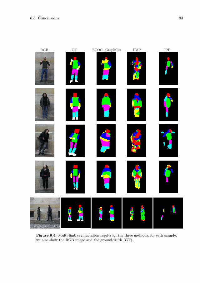
6.5. Conclusions 93

RGB GT ECOC+GraphCut FMP IPP

Figure 6.4: Multi-limb segmentation results for the three methods, for each sample,we also show the RGB image and the ground-truth (GT).

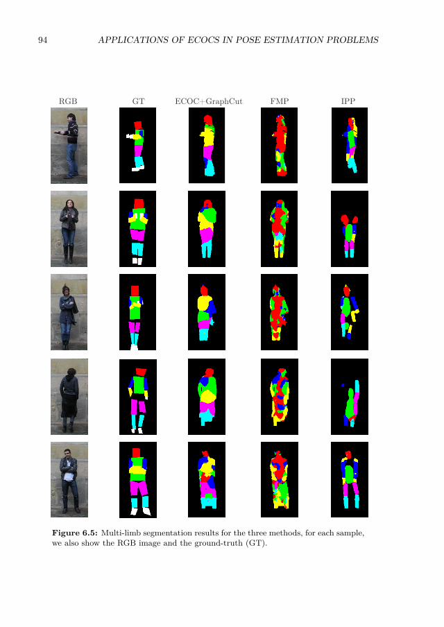
94 APPLICATIONS OF ECOCS IN POSE ESTIMATION PROBLEMS

RGB GT ECOC+GraphCut FMP IPP

Figure 6.5: Multi-limb segmentation results for the three methods, for each sample,we also show the RGB image and the ground-truth (GT).

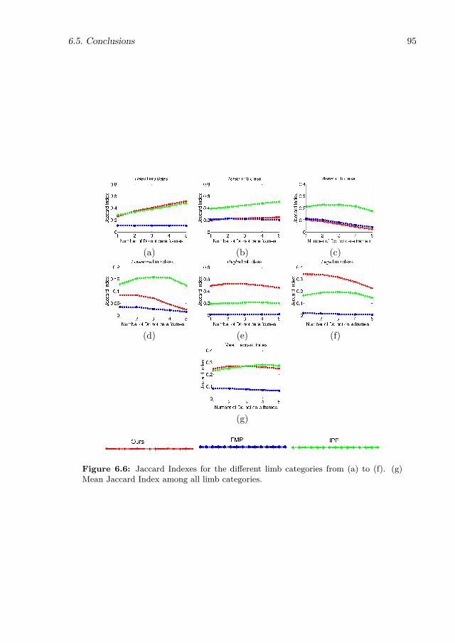
6.5. Conclusions 95

(a) (b) (c)

(d) (e) (f)

(g)

Figure 6.6: Jaccard Indexes for the different limb categories from (a) to (f). (g)Mean Jaccard Index among all limb categories.

96 APPLICATIONS OF ECOCS IN POSE ESTIMATION PROBLEMS

Part IV

Epilogue

97

Chapter 7

Conclusions

Multi-class problems arise very often in real-life situations. In this dissertation we havepresented several ways to treat this multi-class problems by means of Error-Correcting Out-put Codes. In particular, we have focused in the critical aspect of ECOC coding designs,contributing with different problem-dependent coding designs that take into account thestructure of multi-class data, in order to optimize the ECOC coding design to the multi-class data we proposed two different schemes for genetic optimization. In addition, as shownin earlier chapters of this dissertation we also have presented a new way to represent ECOCcoding designs, which enables to study the error-correcting capabilities between pairs ofclasses. Enabled by this novel representation we introduce a discrete matrix factorizationalgorithm to learn ECOC coding matrices.

7.1 Summary of contributionsThe coding step of the ECOC framework is critical for its performance and generalizationcapabilities. In this sense, our contributions in this dissertation are the following:

1. ECOC separability and error-correction: The error-correcting capability of anECOC has always been depicted in literature as a single scalar, which hinders furtheranalyses of the distribution of error-correction between different categories. In thisdissertation we proposed to represent an ECOC by means of its separability matrixand use very simple heuristics to exploit the distribution of error-correction amongpairs of classes to outperform state-of-the-art results.

2. Minimal ECOC Coding Design: We proposed to define the lower bound of anECOC design in terms of the number of binary problems embedded in the codingdesign. We showed that even with a very reduced number of binary classifiers we canobtain comparable results to state-of-the-art coding designs.

3. Genetic Optimization of Minimal ECOCs: Although showing a high perfor-mance, Minimal ECOCs are bounded in terms of generalization capabilities due tothe reduced number of classifiers. In this sense, we proposed to use a Genetic Al-gorithm to optimize the Minimal ECOC coding configuration and obtain a MinimalECOC coding matrix with high generalization capabilities.

4. ECOC-Compliant Genetic Algorithm: Standard Genetic Algorithm use crossoverand mutation operators that treat individuals as binary strings. This operators do not

99

100 CONCLUSIONS

take into account the constraints of the ECOC framework and can lead to poor opti-mization schemes. In this dissertation we proposed to redefine the standard crossoverand mutation operators in order to take into account the constraints of the ECOCframework. In addition we also proposed and operator to dynamically adapt the codelength of the ECOC during the training process. This redefinition of operators led tovery satisfying results in terms of classification performance as a function of the modelcomplexity.

5. Error-Correcting Factorization: Empowered by the novel representation of anECOC as its Separability Matrix we proposed to obtain an estimated Separabilitymatrix from data using very simple statistics and use the proposed Error-CorrectingFactorization to factorize the estimated Separability matrix into a discrete ECOCcoding matrix that distributes error-correcting to those classes that are more prone toerrors.

6. Applications in Human Pose Recovery: As a particular application, in thisdissertation we applied the ECOC framework in the challenging problem of HumanPose Recovery and obtain very satisfying results in comparison with state-of-the-artworks. In addition we proposed the HuPBA 8k+ dataset, the biggest dataset forHuman Pose Recovery in still images.

To conclude, in this dissertation we have defined novel problem dependent-design forthe ECOC coding step that take into account the structure of the multi-class data in orderto obtain models with high generalization performance with a reduced computational cost.In addition, we also presented a novel way to represent an analyze ECOC matrices thatexploits the pair-wise error-correcting capabilities of an ECOC. The techniques obtain highgeneralization performance with a small code length, solving several multi-class real worldproblems like human pose recovery, face recognition or traffic sign categorization.

7.2 Future workAs lines of future research with potential impact we highlight the idea of error-correctingallocation. From a theoretical perspective this dissertation opens a wide set of questionsabout the distribution of error-correction of an ECOC design. While earlier state-of-the-artworks proposed to allocate the error-correcting capabilities to those categories which areeasily separable, we showed how by allocating error-correction to those classes prone to beconfused we outperform state-of-the-art results. However, we consider that a best of bothworlds solution can be interesting to pursue.

In regards to the proposed Error-Correcting Factorization one could potentially regularizethe factorization problem in order to obtain sparse results or additional regularizations (i.e.nuclear norms). In addition, it would be very interesting to couple the ECF problem withthe problem of learning the binary classifiers in order to obtain a joint optimization problemthat obtains high generalization performance.

Moreover, the problem posed by ECF (matrix factorization in binary terms) does not onlyaffect ECOC coding designs, but could impact other areas like Non-negative Matrix Factor-ization, Topic Learning, etc. In particular, the proposed ECF approach could be embeddedin other classifiers that use codewords as their class outputs, for example, ConvolutionalNeural Networks.

For the particular application of Pose Recovery, the contextual relationship between partsplay a very important role in prediction. In this sense, we consider that encoding contextualrelationship between body parts by means of stacking outputs of several ECOC classifierscould dramatically boost performance.

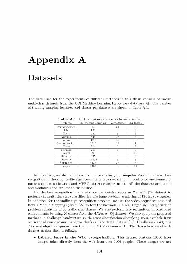
Appendix A

Datasets

The data used for the experiments of different methods in this thesis consists of twelvemulti-class datasets from the UCI Machine Learning Repository database [8]. The numberof training samples, features, and classes per dataset are shown in Table A.1.

Table A.1: UCI repository datasets characteristics.Problem #Training samples #Features #Classes

Dermathology 366 34 6Iris 150 4 3Ecoli 336 8 8Vehicle 846 18 4Wine 178 13 3

Segmentation 2310 19 7Glass 214 9 7

Thyroid 215 5 3Vowel 990 10 11Balance 625 4 3Shuttle 14500 9 7Satimage 4435 36 6Yeast 1484 8 10

In this thesis, we also report results on five challenging Computer Vision problems: facerecognition in the wild, traffic sign recognition, face recognition in controlled environments,music scores classification, and MPEG objects categorization. All the datasets are publicand available upon request to the author.

For the face recognition in the wild we use Labeled Faces in the Wild [74] dataset toperform the multi-class face classification of a large problem consisting of 184 face categories.In addition, for the traffic sign recognition problem, we use the video sequences obtainedfrom a Mobile Mapping System [27] to test the methods in a real traffic sign categorizationproblem consisting of 36 traffic sign classes. We also perform face recognition in controlledenvironments by using 20 classes from the ARFaces [95] dataset. We also apply the proposedmethods in challenge handwritten music score classification classifying seven symbols fromold scanned music scores, using the cleafs and accidental dataset [56]. Finally we classify the70 visual object categories from the public MPEG7 dataset [1]. The characteristics of eachdataset as described as follows.

• Labeled Faces in the Wild categorization: This dataset contains 13000 facesimages taken directly from the web from over 1400 people. These images are not

101

102 DATASETS

constrained in terms of pose, light, occlusions or any other relevant factor. For thepurpose of this experiment we used a specific subset, taking only the categories whichat least have four or more examples, having a total of 184 face categories. Finally, inorder to extract relevant features from the images, we apply an Incremental PrincipalComponent Analysis procedure [75], keeping 99.8% of the information. An exampleof face images is shown in Figure A.1.

Figure A.1: Labeled Faces in the Wild dataset.

• Traffic sign categorization: For this second computer vision experiment, we usethe video sequences obtained from the Mobile Mapping System of [27] to test the Evo-lutionary Minimal ECOC methodology on a real traffic sign categorization problem.In this system, the position and orientation of the different traffic signs are measuredwith video cameras fixed on a moving vehicle. The system has a stereo pair of cali-brated cameras, which are synchronized with a GPS/INS system. The result of theacquisition step is a set of stereo-pairs of images with their position and orientationinformation. From this system, a set of 36 circular and triangular traffic sign classesare obtained. Some categories from this data set are shown in Figure A.2. The datasetcontains a total of 3481 samples of size 32×32, filtered using the Weickert anisotropicfilter, masked to exclude the background pixels, and equalized to prevent the effectsof illumination changes. These feature vectors are then projected into a 100 featurevector by means of PCA.

Figure A.2: Traffic sign classes.

• ARFaces classification: The ARFace database [95] is composed of 26 face imagesfrom 126 different subjects (70 men and 56 women). The images have uniform whitebackground. The database has two sets of images from each person, acquired in twodifferent sessions, with the following structure: one sample of neutral frontal images,three samples with strong changes in the illumination, two samples with occlusions

103

(scarf and glasses), four images combining occlusions and illumination changes, andthree samples with gesture effects. One example of each type is plotted in Figure A.3.For this experiment, we selected all the samples from 20 different categories (persons).

Figure A.3: ARFaces dataset classes. Examples from a category with neutral, smile,anger, scream expressions, wearing sun glasses, wearing sunglasses and left light on,wearing sun glasses and right light on, wearing scarf, wearing scarf and left light on,and wearing scarf and right light on.

• Clefs and accidental dataset categorization:The dataset of clefs and accidental [56] is obtained from a collection of modern andold musical scores (19th century) of the Archive of the Seminar of Barcelona. Thedataset contains a total of 4098 samples among seven different types of clefs and acci-dental from 24 different authors. The images have been obtained from original imagedocuments using a semi-supervised segmentation approach [56]. The main difficultyof this dataset is the lack of a clear class separability because of the variation of writerstyles and the absence of a standard notation. A pair of segmented samples for each ofthe seven classes showing the high variability of clefs and accidental appearance fromdifferent authors can be observed in Figure A.4 (a). An example of an old musicalscore used to obtain the data samples are shown in Figure A.4(b). The object imagesare described using the Blurred Shape Model descriptor [45].

• MPEG7 categorization: The MPEG7 dataset contains 70 classes with 20 instancesper class, which represents a total of 1400 object images. All samples are describedusing the Blurred Shape Model descriptor [45]. A couple of samples for some categoriesof this dataset are shown in Figure A.5.

104 DATASETS

(a)

(b)

Figure A.4: (a) Object samples. (b) Old music score.

Figure A.5: MPEG7 samples.

Appendix B

Publications

The following publications are a consequence of the research carried out during the elabora-tion of this thesis and give an idea of the progression that has been achieved.

B.1 Journals• Error-Correcting Factorization, Bautista, Miguel Ángel and De la Torre, Fernando

and Pujol, Oriol, and Escalera, Sergio. IEEE Transactions on Pattern Analysis andMachine Intelligence. Under Review, 2015.

• AGesture Recognition System for Detecting Behavioral Patterns of ADHD,Bautista, Miguel Ángel and Hernández-Vela, Antonio and Escalera, Sergio and Igual,Laura and Pujol, Oriol and Moya, Josep and Violant, Verónica and Anguera, MaríaTeresa, IEEE Transactions on System, Man and Cybernetics, Part B. In Press, 2015.

• On the design of an ECOC-compliant genetic algorithm, Bautista, MiguelÁngel and Escalera, Sergio and Baró, Xavier and Pujol, Oriol, Pattern Recognition,47, 2, 865–884, 2013, Elsevier.

• HuPBA 8k+: Dataset and ECOC-GraphCut based Segmentation of Hu-man Limbs, Sanchez, Daniel and Bautista, Miguel Ángel and Escalera, and Sergio.Neurocomputing, 2014, Elsevier.

• Minimal Design of Error-Correcting Output Codes, Bautista, Miguel Ángeland Escalera, Sergio and Baró, Xavier and Radeva, Petia and Vitriá, Jordi and Pujol,Oriol. Pattern Recognition Letters, 33, 6, 693–702, 2011, Elsevier.

• Probability-based dynamic time warping and bag-of-visual-and-depth-wordsfor human gesture recognition in rgb-d, Hernández-Vela, Antonio and Bautista,Miguel Ángel and Perez-Sala, Xavier and Ponce-López, Víctor and Escalera, Sergioand Baró, Xavier and Pujol, Oriol and Angulo, Cecilio. Pattern Recognition Letters,50, 112-121, 2014, Elsevier.

B.2 International Conferences and Workshops• Introducing the separability matrix for error correcting output codes cod-ing. Bautista, Miguel and Pujol, Oriol and Baró, Xavier and Escalera, Sergio. Mul-tiple Classifier Systems, 227–236, 2011, Springer.

105

106 PUBLICATIONS

• On the Design of Low Redundancy Error-Correcting Output Codes. Bautista,Miguel and Escalera, Sergio and Baró, Xavier and Pujol, Oriol and Vitria, Jordi andRadeva, Petia. Ensembles in Machine Learning Applications, 21–38, 2011, Springer.

• Compact evolutive design of error-correcting output codes. Bautista, MAand Baro, X and Pujol, O and Radeva, P and Vitria, J and Escalera, S. EuropeanConference on Machine Learning Workshops, 119–128, 2010, LNCS.

• Probability-based Dynamic TimeWarping for Gesture Recognition on RGB-D data. Bautista, Miguel Angel and Hernández-Vela, Antonio and Ponce, Victor andPerez-Sala, Xavier and Baró, Xavier and Pujol, Oriol and Angulo, Cecilio and Es-calera, Sergio. International Conference on Pattern Recogntion Workshops, Advancesin Depth Image Analysis and Applications, 126–135, 2012, LNCS 7854 - Springer.

• A genetic inspired optimization for ECOC. Bautista, Miguel Ángel and Escalera,Sergio and Baró, Xavier and Pujol, Oriol. Structural, Syntactic, and Statistical Pat-tern Recognition, 743–751, 2012, Springer Berlin Heidelberg.

• BoVDW: Bag-of-Visual-and-Depth-Words for gesture recognition. Hernández-Vela, Antonio and Bautista, Miguel Angel and Perez-Sala, Xavier and Ponce, Victorand Baró, Xavier and Pujol, Oriol and Angulo, Cecilio and Escalera, Sergio. 21stInternational Conference on Pattern Recognition (ICPR), 2012, 449–452, 2012, IEEE.

• Human body segmentation with multi-limb error-correcting output codesdetection and graph cuts optimization. Sánchez, Daniel and Ortega, Juan Carlosand Bautista, Miguel Ángel and Escalera, Sergio. Pattern Recognition and ImageAnalysis, 50–58, 2013, Springer Berlin Heidelberg.

• Chalearn looking at people challenge 2014: Dataset and results. Escalera,Sergio and Bar, X and Gonzlez, J and Bautista, Miguel A and Madadi, Meysam andReyes, Miguel and Ponce, V and Escalante, Hugo J and Shotton, Jamie and Guyon,Isabelle. IEEE European Conference Computer Vision Looking At People Workshop,2014.

• Learning To Segment Humans By Stacking Their Body Parts. Puertas, Eloiand Bautista, MA and Sanchez, Daniel and Escalera, Sergio and Pujol, Oriol. IEEEEuropean Conference Computer Vision Looking At People Workshop, 2014.

BIBLIOGRAPHY 107

Bibliography[1] http://www.cis.temple.edu/latecki/research.html.

[2] S. Agarwal, J. Wills, L. Cayton, G. Lanckriet, D. J. Kriegman, and S. Belongie. Gen-eralized non-metric multidimensional scaling. In International Conference on ArtificialIntelligence and Statistics, pages 11–18, 2007.

[3] E. Allwein, R. Schapire, and Y. Singer. Reducing multiclass to binary: A unifyingapproach for margin classifiers. JMLR, 1:113–141, 2002.

[4] E. L. Allwein, R. E. Schapire, Y. Singer, and P. Kaelbling. Reducing multiclass tobinary: A unifying approach for margin classifiers. Journal of Machine Learning Re-search, 1:113–141, 2000.

[5] E. Alpaydin and E. Mayoraz. Learning error-correcting output codes from data. In Ar-tificial Neural Networks, 1999. ICANN 99. Ninth International Conference on (Conf.Publ. No. 470), volume 2, pages 743 –748 vol.2, 1999.

[6] M. Andriluka, S. Roth, and B. Schiele. Pictorial structures revisited: People detectionand articulated pose estimation. In Computer Vision and Pattern Recognition, 2009.CVPR 2009. IEEE Conference on, pages 1014–1021. IEEE, 2009.

[7] M. Ángel Bautista, S. Escalera, X. Baró, and O. Pujol. On the design of an ecoc-compliant genetic algorithm. Pattern Recognition, 47(2):865 – 884, 2013.

[8] A. Asuncion and D. Newman. UCI machine learning repository.http://www.ics.uci.edu/∼mlearn/MLRepository.html, 2007. University of Cali-fornia, Irvine, School of Information and Computer Sciences.

[9] S. Baluja and R. Caruana. Removing the genetics from the standard genetic algorithm.In A. Prieditis and S. Russel, editors, The Int. Conf. on Machine Learning 1995, pages38–46, San Mateo, CA, 1995. Morgan Kaufmann Publishers.

[10] M. Bautista, S. Escalera, X. Baró, P. Radeva, J. Vitriá, and O. Pujol. Minimal designof error-correcting output codes. Pattern Recognition Letters. In press., 2011.

[11] M. Á. Bautista, S. Escalera, X. Baró, and O. Pujol. On the design of an ecoc-compliantgenetic algorithm. Pattern Recognition, 47(2):865–884, 2014.

[12] M. A. Bautista, S. Escalera, X. Baró, P. Radeva, J. Vitriá, and O. Pujol. Minimaldesign of error-correcting output codes. Pattern Recogn. Lett., 33(6):693–702, Apr.2012.

[13] U. R. Beierholm, S. R. Quartz, and L. Shams. Bayesian priors are encoded indepen-dently from likelihoods in human multisensory perception. Journal of vision, 9(5):23,2009.

[14] S. Belongie, J. Malik, and J. Puzicha. Shape context: A new descriptor for shapematching and object recognition. In NIPS, volume 2, page 3, 2000.

[15] Y. Bengio, R. De Mori, G. Flammia, and R. Kompe. Global optimization of a neu-ral network-hidden markov model hybrid. Neural Networks, IEEE Transactions on,3(2):252–259, 1992.

108 PUBLICATIONS

[16] Y. Bengio, P. Simard, and P. Frasconi. Learning long-term dependencies with gradientdescent is difficult. Neural Networks, IEEE Transactions on, 5(2):157–166, 1994.

[17] C. M. Bishop. Pattern recognition and machine learning. springer, 2006.

[18] B. E. Boser, I. M. Guyon, and V. N. Vapnik. A training algorithm for optimal marginclassifiers. In Proceedings of the fifth annual workshop on Computational learningtheory, pages 144–152. ACM, 1992.

[19] L. Bourdev and J. Malik. Poselets: Body part detectors trained using 3d human poseannotations. In ICCV, pages 1365–1372. IEEE, 2009.

[20] S. Boyd and L. Vandenberghe. Convex optimization. Cambridge university press, 2009.

[21] S. Boyd and L. Xiao. Least-squares covariance matrix adjustment. SIAM Journal onMatrix Analysis and Applications, 27(2):532–546, 2005.

[22] Y. Boykov and G. Funka-Lea. Graph cuts and efficient nd image segmentation. Inter-national Journal of Computer Vision, 70(2):109–131, 2006.

[23] Y. Boykov and V. Kolmogorov. Computing geodesics and minimal surfaces via graphcuts. In CVPR, pages 26–33, 2003.

[24] Y. Boykov and V. Kolmogorov. An experimental comparison of min-cut/max-flow al-gorithms for energy minimization in vision. Pattern Analysis and Machine Intelligence,IEEE Transactions on, 26(9):1124–1137, 2004.

[25] Y. Boykov, O. Veksler, and R. Zabih. Fast approximate energy minimization via graphcuts. Pattern Analysis and Machine Intelligence, IEEE Transactions on, 23(11):1222–1239, 2001.

[26] L. Breiman. Random forests. Machine learning, 45(1):5–32, 2001.

[27] J. Casacuberta, J. Miranda, M. Pla, S. Sanchez, A.Serra, and J.Talaya. On the ac-curacy and performance of the GeoMobil system. In International Society for Pho-togrammetry and Remote Sensing, 2004.

[28] L. Cayton and S. Dasgupta. Robust euclidean embedding. In Proceedings of the 23rdinternational conference on machine learning, pages 169–176. ACM, 2006.

[29] C.-C. Chang and C.-J. Lin. LIBSVM: A library for support vector machines. ACMTransactions on Intelligent Systems and Technology, 2:27:1–27:27, 2011. Softwareavailable at http://www.csie.ntu.edu.tw/~cjlin/libsvm.

[30] Y.-T. Chen and C.-S. Chen. Fast human detection using a novel boosted cascadingstructure with meta stages. Image Processing, IEEE Transactions on, 17(8):1452–1464,2008.

[31] T. F. Coleman and Y. Li. A reflective newton method for minimizing a quadraticfunction subject to bounds on some of the variables. SIAM Journal on Optimization,6(4):1040–1058, 1996.

[32] K. Crammer and Y. Singer. Improved output coding for classification using continuousrelaxation. In In Advances in Neural Information Processing Systes 13 (NIPS*00, 2001.

BIBLIOGRAPHY 109

[33] K. Crammer and Y. Singer. On the algorithmic implementation of multiclass kernel-based vector machines. The Journal of Machine Learning Research, 2:265–292, 2002.

[34] K. Crammer and Y. Singer. On the learnability and design of output codes for multi-class problems. In Machine Learning, volume 47, pages 201–233, 2002.

[35] N. Dalal and B. Triggs. Histograms of oriented gradients for human detection. InCVPR, volume 1, pages 886 –893 vol. 1, 2005.

[36] F. De la Torre. A least-squares framework for component analysis. IEEE TransactionsPattern Analysis and Machine Intelligence (PAMI), 34(6):1041–1055, 2012.

[37] F. De la Torre, J. K. Hodgins, J. Montano, and S. Valcarcel. Detailed human dataacquisition of kitchen activities: the cmu-multimodal activity database (cmu-mmac).Technical report, RI-TR-08-22h, CMU, 2008.

[38] J. Demsar. Statistical comparisons of classifiers over multiple data sets. JMLR, 7:1–30,2006.

[39] T. Dietterich and G. Bakiri. Solving multiclass learning problems via error-correctingoutput codes. In Journal of Artificial Intelligence Research, volume 2, pages 263–286,1995.

[40] P. E. Downing, Y. Jiang, M. Shuman, and N. Kanwisher. A cortical area selective forvisual processing of the human body. Science, 293(5539):2470–2473, 2001.

[41] R. Duin and E. Pekalska. The science of pattern recognition; achievements and per-spectives. In W. Duch and J. Mandziuk, editors, Challenges for Computational Intel-ligence, Studies in Computational Intelligence, volume 63, pages 221–259, 2007.

[42] R. P. Duin and E. Pekalska. The science of pattern recognition. achievements andperspectives. In Challenges for computational intelligence, pages 221–259. Springer,2007.

[43] M. Enzweiler and D. M. Gavrila. Monocular pedestrian detection: Survey andexperiments. Pattern Analysis and Machine Intelligence, IEEE Transactions on,31(12):2179–2195, 2009.

[44] R. Epstein and N. Kanwisher. A cortical representation of the local visual environment.Nature, 392(6676):598–601, 1998.

[45] S. Escalera, A. Fornes, O. Pujol, P. Radeva, G. Sanchez, and J. Llados. Blurredshape model for binary and grey-level symbol recognition. Pattern Recognition Letters,30:1424–1433, 2009.

[46] S. Escalera, J. Gonzàlez, X. Baró, M. Reyes, O. Lopes, I. Guyon, V. Athitsos, andH. J. Escalante. Multi-modal gesture recognition challenge 2013: Dataset and results.ChaLearn Multi-modal Gesture Recognition Grand Challenge and Workshop, 15th ACMInternational Conference on Multimodal Interaction, pages 445–452, 2013.

[47] S. Escalera, O. Pujol, and P.Radeva. On the decoding process in ternary error-correcting output codes. Transactions in Pattern Analysis and Machine Intelligence,99(1), 2009.

110 PUBLICATIONS

[48] S. Escalera, O. Pujol, and P. Radeva. Ecoc-one: A novel coding and decoding strategy.In Pattern Recognition, 2006. ICPR 2006. 18th International Conference on, volume 3,pages 578 –581, 2006.

[49] S. Escalera, O. Pujol, and P. Radeva. Boosted landmarks and forest ECOC: A novelframework to detect and classify objects in clutter scenes. In Pattern RecognitionLetters, volume 28, pages 1759–1768, 2007.

[50] S. Escalera, O. Pujol, and P. Radeva. On the decoding process in ternary error-correcting output codes. PAMI, 32:120–134, 2010.

[51] S. Escalera, D. M. Tax, O. Pujol, P. Radeva, and R. P. Duin. Subclass problem-dependent design for error-correcting output codes. Pattern Analysis and MachineIntelligence, IEEE Transactions on, 30(6):1041–1054, 2008.

[52] L. J. Eshelman. The chc adaptive search algorithm: How to have safe search whenengaging in nontraditional genetic recombination. In FOGA, pages 265–283, 1990.

[53] M. Everingham, L. Van Gool, C. K. I. Williams, J. Winn, and A. Zisserman. Thepascal visual object classes (voc) challenge. International Journal of Computer Vision,88(2):303–338, June 2010.

[54] P. F. Felzenszwalb and D. P. Huttenlocher. Pictorial structures for object recognition.International Journal of Computer Vision, 61(1):55–79, 2005.

[55] V. Ferrari, M. Marin-Jimenez, and A. Zisserman. Progressive search space reductionfor human pose estimation. In IEEE Conference on Computer Vision and PatternRecognition, 2008.

[56] A. Fornés, J. Lladós, and G. Sánchez. Primitive segmentation in old handwritten musicscores. Graphics Recognition: Ten Years Review and Future Perspectives, 3926:279–290, 2006.

[57] Y. Freund and R. Schapire. A decision-theoretic generalization of on-line learning andan application to boosting. In EuroCOLT, pages 23–37, 1995.

[58] J. Friedman, T. Hastie, and R. Tibshirani. Regularization paths for generalized linearmodels via coordinate descent. Journal of statistical software, 33(1):1, 2010.

[59] K. Fukushima. Neocognitron: A hierarchical neural network capable of visual patternrecognition. Neural networks, 1(2):119–130, 1988.

[60] T. Gao and D. Koller. Discriminative learning of relaxed hierarchy for large-scale visualrecognition. In ICCV, 2011.

[61] T. Gao and D. Koller. Multiclass boosting with hinge loss based on output coding.In Proceedings of the 28th International Conference on Machine Learning (ICML-11),pages 569–576, 2011.

[62] N. Garcia-Pedrajas and C. Fyfe. Evolving output codes for multiclass problems. Evo-lutionary Computation, IEEE Transactions on, 12(1):93 –106, 2008.

[63] A. Globerson, G. Chechik, F. Pereira, and N. Tishby. Euclidean embedding of co-occurrence data. Journal of Machine Learning Research, 8:2265–2295, 2007.

BIBLIOGRAPHY 111

[64] G. Griffin and P. Perona. Learning and using taxonomies for fast visual categorization.In Computer Vision and Pattern Recognition, 2008. CVPR 2008. IEEE Conference on,pages 1–8. IEEE, 2008.

[65] L. Grippo and M. Sciandrone. On the convergence of the block nonlinear gauss–seidelmethod under convex constraints. Operations Research Letters, 26(3):127 – 136, 2000.

[66] N. Guan, D. Tao, Z. Luo, and B. Yuan. Nenmf: an optimal gradient method for nonneg-ative matrix factorization. Signal Processing, IEEE Transactions on, 60(6):2882–2898,2012.

[67] K. He, X. Zhang, S. Ren, and J. Sun. Spatial pyramid pooling in deep convolutionalnetworks for visual recognition. In Computer Vision–ECCV 2014, pages 346–361.Springer, 2014.

[68] A. Hernández-Vela, N. Zlateva, A. Marinov, M. Reyes, P. Radeva, D. Dimov, andS. Escalera. Graph cuts optimization for multi-limb human segmentation in depthmaps. In CVPR, pages 726–732, 2012.

[69] N. J. Higham. Computing the nearest correlation matrix—a problem from finance.IMA journal of Numerical Analysis, 22(3):329–343, 2002.

[70] J. Holland. Adaptation in natural and artificial systems: An analysis with applicationsto biology, control, and artificial intelligence. University of Michigan Press, 1975.

[71] C.-J. Hsieh and I. S. Dhillon. Fast coordinate descent methods with variable selectionfor non-negative matrix factorization. In Proceedings of the 17th ACM SIGKDD inter-national conference on Knowledge discovery and data mining, pages 1064–1072. ACM,2011.

[72] C. Hsu, C. Chang, and C. Lin. A practical guide to support vector classification.Department of CSIE, technical report, 2002.

[73] F. J. Huang and Y. LeCun. Large-scale learning with svm and convolutional forgeneric object categorization. In Computer Vision and Pattern Recognition, 2006IEEE Computer Society Conference on, volume 1, pages 284–291. IEEE, 2006.

[74] G. B. Huang, M. Ramesh, T. Berg, and E. L. Miller. Labeled faces in the wild:A database for studying face recognition in unconstrained environments. TechnicalReport University of Massachusets Amherst, 07-49, October 2007.

[75] W. Hwang, J. Weng, and Y. Zhang. Candid covariance-free incremental principalcomponent analysis. IEEE Transactions on Pattern Analysis and Machine Intelligence,25(8):1034–1040, 2003.

[76] A. Jain, R. Duin, and J. Mao. Statistical pattern recognition: A review. In IEEETransactions on Pattern Analysis and Machine Intelligence, volume 22, 2000.

[77] S. Johnson and M. Everingham. Clustered pose and nonlinear appearance modelsfor human pose estimation. In Proceedings of the British Machine Vision Conference,2010. doi:10.5244/C.24.12.

[78] N. Kanwisher, J. McDermott, and M. M. Chun. The fusiform face area: a module inhuman extrastriate cortex specialized for face perception. The Journal of Neuroscience,17(11):4302–4311, 1997.

112 PUBLICATIONS

[79] H. Kim and H. Park. Nonnegative matrix factorization based on alternating nonneg-ativity constrained least squares and active set method. SIAM Journal on MatrixAnalysis and Applications, 30(2):713–730, 2008.

[80] R. Kohavi. A study of cross-validation and bootstrap for accuracy estimation andmodel selection. In IJCAI, pages 1137–1145, 1995.

[81] E. B. Kong and T. G. Dietterich. Error-correcting output coding corrects bias andvariance. In ICML, pages 313–321, 1995.

[82] A. Krizhevsky, I. Sutskever, and G. E. Hinton. Imagenet classification with deepconvolutional neural networks. In Advances in neural information processing systems,pages 1097–1105, 2012.

[83] J. B. Kruskal. Nonmetric multidimensional scaling: a numerical method. Psychome-trika, 29(2):115–129, 1964.

[84] L. I. Kuncheva and C. J. Whitaker. Measures of diversity in classifier ensembles andtheir relationship with the ensemble accuracy. Machine learning, 51(2):181–207, 2003.

[85] I. Laptev, M. Marszalek, C. Schmid, and B. Rozenfeld. Learning realistic humanactions from movies. In Computer Vision and Pattern Recognition, 2008. CVPR 2008.IEEE Conference on, pages 1–8. IEEE, 2008.

[86] Y. LeCun and Y. Bengio. Convolutional networks for images, speech, and time series.The handbook of brain theory and neural networks, 3361(10), 1995.

[87] Y. LeCun, L. Jackel, L. Bottou, A. Brunot, C. Cortes, J. Denker, H. Drucker, I. Guyon,U. Muiller, E. Sackinger, et al. Comparison of learning algorithms for handwritten digitrecognition. In International Conference on Artificial Neural Networks, pages 53–60,1995.

[88] C.-J. Lin. Projected gradient methods for nonnegative matrix factorization. Neuralcomputation, 19(10):2756–2779, 2007.

[89] A. C. Lorena and A. C. P. L. F. Carvalho. Evolutionary design of multiclass supportvector machines. J. Intell. Fuzzy Syst., 18:445–454, October 2007.

[90] A. C. Lorena and A. C. de Carvalho. Evolutionary tuning of svm parameter values inmulticlass problems. Neurocomputing, 71(16-18):3326 – 3334, 2008.

[91] D. G. Lowe. Object recognition from local scale-invariant features. In Computer vision,1999. The proceedings of the seventh IEEE international conference on, volume 2, pages1150–1157. Ieee, 1999.

[92] W. J. Ma, J. M. Beck, P. E. Latham, and A. Pouget. Bayesian inference with proba-bilistic population codes. Nature neuroscience, 9(11):1432–1438, 2006.

[93] J. Malick. A dual approach to semidefinite least-squares problems. SIAM Journal onMatrix Analysis and Applications, 26(1):272–284, 2004.

[94] M. Marszalek and C. Schmid. Constructing category hierarchies for visual recognition.In Computer Vision–ECCV 2008, pages 479–491. Springer, 2008.

BIBLIOGRAPHY 113

[95] A. Martinez and R. Benavente. The AR face database. In Computer Vision CenterTechnical Report #24, 1998.

[96] P. Miettinen, T. Mielikainen, A. Gionis, G. Das, and H. Mannila. The discrete basisproblem. Knowledge and Data Engineering, IEEE Transactions on, 20(10):1348–1362,2008.

[97] K. Mikolajczyk, C. Schmid, and A. Zisserman. Human detection based on a prob-abilistic assembly of robust part detectors. In Computer Vision-ECCV 2004, pages69–82. Springer, 2004.

[98] I. Mukherjee and R. E. Schapire. A theory of multiclass boosting. The Journal ofMachine Learning Research, 14(1):437–497, 2013.

[99] Y. Nesterov. Efficiency of coordinate descent methods on huge-scale optimizationproblems. SIAM Journal on Optimization, 22(2):341–362, 2012.

[100] N. J. Nilsson. Learning machines: foundations of trainable pattern-classifying systems.McGraw-Hill, 1965.

[101] OSU-SVM-TOOLBOX. http://svm.sourceforge.net/.

[102] A. Passerini, M. Pontil, and P. Frasconi. New results on error correcting output codesof kernel machines. Neural Networks, IEEE Transactions on, 15(1):45–54, 2004.

[103] M. Pelikan, D. E. Goldberg, and E. Cantú-Paz. Learning machines. In McGraw-Hill,1965.

[104] R. Polikar. Ensemble based systems in decision making. Circuits and Systems Maga-zine, IEEE, 6(3):21–45, 2006.

[105] O. Pujol, S. Escalera, and P. Radeva. An incremental node embedding technique forerror correcting output codes. Pattern Recognition, 41(2):713 – 725, 2008.

[106] O. Pujol, P. Radeva, and J. Vitrià. Discriminant ecoc: A heuristic method for applica-tion dependent design of error correcting output codes. In Trans. on PAMI, volume 28,pages 1001–1007, 2006.

[107] J. R. Quinlan. Induction of decision trees. Machine learning, 1(1):81–106, 1986.

[108] D. Ramanan. Learning to parse images of articulated bodies. In Advances in neuralinformation processing systems, pages 1129–1136, 2006.

[109] D. Ramanan, D. Forsyth, and A. Zisserman. Tracking people by learning their ap-pearance. PAMI, 29(1):65 –81, jan. 2007.

[110] P. Richtárik and M. Takávc. Iteration complexity of randomized block-coordinatedescent methods for minimizing a composite function. Mathematical Programming,144(1-2):1–38, 2014.

[111] R. Rifkin and A. Klautau. In defense of one-vs-all classification. JMLR, 5:101–141,2004.

[112] D. L. Rohde. Methods for binary multidimensional scaling. Neural Computation,14(5):1195–1232, 2002.

114 PUBLICATIONS

[113] F. Rosenblatt. Principles of neurodynamics. 1962.

[114] C. Rother, V. Kolmogorov, and A. Blake. "grabcut": interactive foreground extractionusing iterated graph cuts. ACM Trans. Graph., 23(3):309–314, Aug. 2004.

[115] D. E. Rumelhart, G. E. Hinton, and R. J. Williams. Learning internal representationsby error propagation. Technical report, DTIC Document, 1985.

[116] M. J. Saberian and N. Vasconcelos. Multiclass boosting: Theory and algorithms. InAdvances in Neural Information Processing Systems, pages 2124–2132, 2011.

[117] D. Sanchez, M. Á. Bautista, and S. Escalera. Hupba 8k+: Dataset and ecoc-graphcutbased segmentation of human limbs. Neurocomputing, 2014.

[118] B. Sapp, C. Jordan, and B. Taskar. Adaptive pose priors for pictorial structures. InComputer Vision and Pattern Recognition (CVPR), 2010 IEEE Conference on, pages422–429. IEEE, 2010.

[119] R. E. Schapire. Using output codes to boost multiclass learning problems. In ICML,volume 97, pages 313–321, 1997.

[120] C. Schuldt, I. Laptev, and B. Caputo. Recognizing human actions: a local svm ap-proach. In Pattern Recognition, 2004. ICPR 2004. Proceedings of the 17th InternationalConference on, volume 3, pages 32–36. IEEE, 2004.

[121] P. Simard, Y. LeCun, and J. S. Denker. Efficient pattern recognition using a newtransformation distance. In Advances in Neural Information Processing Systems 5,NIPS 1992, pages 50–58. Morgan Kaufmann Publishers Inc., 1992.

[122] P. Simeone, C. Marrocco, and F. Tortorella. Design of reject rules for ecoc classificationsystems. Pattern Recognition, 45(2):863 – 875, 2012.

[123] D. F. Specht. Probabilistic neural networks. Neural networks, 3(1):109–118, 1990.

[124] Y. Tang. Deep learning using linear support vector machines. arXiv preprintarXiv:1306.0239, 2013.

[125] T.Hastie and R.Tibshirani. Classification by pairwise grouping. NIPS, 26:451–471,1998.

[126] D. Tran and D. Forsyth. Improved human parsing with a full relational model. InComputer Vision–ECCV 2010, pages 227–240. Springer, 2010.

[127] P. Tseng. Convergence of a block coordinate descent method for nondifferentiableminimization. Journal of optimization theory and applications, 109(3):475–494, 2001.

[128] W. Utschick and W. Weichselberger. Stochastic organization of output codes in mul-ticlass learning problems. In Neural Computation, volume 13, pages 1065–1102, 2004.

[129] V. N. Vapnik and V. Vapnik. Statistical learning theory, volume 1. Wiley New York,1998.

[130] V. Vineet, J. Warrell, L. Ladicky, and P. Torr. Human instance segmentation fromvideo using detector-based conditional random fields. In BMVC, 2011.

BIBLIOGRAPHY 115

[131] P. Viola and M. Jones. Rapid object detection using a boosted cascade of simplefeatures. In CVPR, volume 1, 2001.

[132] S. Watanabe. Pattern Recognition: Human and Mechanical. John Wiley & Sons, Inc.,New York, NY, USA, 1985.

[133] K. Q. Weinberger, J. Blitzer, and L. K. Saul. Distance metric learning for large marginnearest neighbor classification. In Advances in neural information processing systems,pages 1473–1480, 2005.

[134] T. H. Weisswange, C. A. Rothkopf, T. Rodemann, and J. Triesch. Bayesian cueintegration as a developmental outcome of reward mediated learning. PLoS One,6(7):e21575, 2011.

[135] J. Weston, C. Watkins, et al. Support vector machines for multi-class pattern recog-nition. In ESANN, volume 99, pages 219–224, 1999.

[136] T. Windeatt and R. Ghaderi. Coding and decoding for multi-class learning problems.In Information Fusion, volume 4, pages 11–21, 2003.

[137] J. Yang, K. Yu, Y. Gong, and T. Huang. Linear spatial pyramid matching using sparsecoding for image classification. In Computer Vision and Pattern Recognition, 2009.CVPR 2009. IEEE Conference on, pages 1794–1801. IEEE, 2009.

[138] Y. Yang and D. Ramanan. Articulated pose estimation with flexible mixtures-of-parts.In IEEE Conference on Computer Vision and Pattern Recognition, pages 1385–1392.IEEE, 2011.

[139] Y. Yang and D. Ramanan. Articulated human detection with flexible mixtures-of-parts. 2012.

[140] B. T. Yeo, F. M. Krienen, J. Sepulcre, M. R. Sabuncu, D. Lashkari, M. Hollinshead,J. L. Roffman, J. W. Smoller, L. Zöllei, J. R. Polimeni, et al. The organization ofthe human cerebral cortex estimated by intrinsic functional connectivity. Journal ofneurophysiology, 106(3):1125–1165, 2011.

[141] X. Zhang, L. Liang, and H.-Y. Shum. Spectral error correcting output codes for efficientmulticlass recognition. In Computer Vision, 2009 IEEE 12th International Conferenceon, pages 1111–1118, Sept 2009.

[142] B. Zhao and E. P. Xing. Sparse output coding for large-scale visual recognition. InComputer Vision and Pattern Recognition (CVPR), 2013 IEEE Conference on, pages3350–3357. IEEE, 2013.

[143] G. Zhong and M. Cheriet. Adaptive error-correcting output codes. In Proceedings ofthe Twenty-Third international joint conference on Artificial Intelligence, pages 1932–1938. AAAI Press, 2013.

[144] G. Zhong, K. Huang, and C.-L. Liu. Joint learning of error-correcting output codes anddichotomizers from data. Neural Computing and Applications, 21(4):715–724, 2012.

[145] J. Zhou, H. Peng, and C. Y. Suen. Data-driven decomposition for multi-class classifi-cation. Pattern Recognition, 41(1):67 – 76, 2008.

116 PUBLICATIONS

[146] J. D. Zhou, X. D. Wang, H. J. Zhou, J. M. Zhang, and N. Jia. Decoding design based onposterior probabilities in ternary error-correcting output codes. Pattern Recognition,45(4):1802 – 1818, 2012.

[147] J. Zhu, H. Zou, S. Rosset, and T. Hastie. Multi-class adaboost. Statistics and Its,2009.

[148] Q. Zhu, M.-C. Yeh, K.-T. Cheng, and S. Avidan. Fast human detection using a cascadeof histograms of oriented gradients. In Computer Vision and Pattern Recognition, 2006IEEE Computer Society Conference on, volume 2, pages 1491–1498. IEEE, 2006.