NBER WORKING PAPER SERIES

LEARNING ENTREPRENEURSHIP FROM OTHER ENTREPRENEURS?

Luigi GuisoLuigi Pistaferri

Fabiano Schivardi

Working Paper 21775http://www.nber.org/papers/w21775

NATIONAL BUREAU OF ECONOMIC RESEARCH1050 Massachusetts Avenue

Cambridge, MA 02138December 2015

We thank Michael Fritsch, Ed Glaeser, Vernon Henderson, Mirjam Van Praag, Antoinette Schoar, MattTurner, participants to the NBER 2014 Summer Institute, the 5th HEC Workshop on Entrepreneurship- Entrepreneurial Finance, the Second CEPR European Workshop on Entrepreneurship Economics andthe 5th IZA Workshop on Entrepreneurship Research for useful comments and suggestions. Financialsupport from the Regione Sardegna, Legge 7/2007- grant CRP 26133 is gratefully acknowledged.The views expressed herein are those of the authors and do not necessarily reflect the views of theNational Bureau of Economic Research.

NBER working papers are circulated for discussion and comment purposes. They have not been peer-reviewed or been subject to the review by the NBER Board of Directors that accompanies officialNBER publications.

© 2015 by Luigi Guiso, Luigi Pistaferri, and Fabiano Schivardi. All rights reserved. Short sectionsof text, not to exceed two paragraphs, may be quoted without explicit permission provided that fullcredit, including © notice, is given to the source.

Learning Entrepreneurship From Other Entrepreneurs?Luigi Guiso, Luigi Pistaferri, and Fabiano SchivardiNBER Working Paper No. 21775December 2015JEL No. J24,M13,R11

ABSTRACT

We document that individuals who grew up in areas with high density of firms are more likely, asadults, to become entrepreneurs, controlling for the density of firms in their current location. Conditionalon becoming entrepreneurs, the same individuals are also more likely to be successful entrepreneurs,as measured by business income or firm productivity. Strikingly, firm density at entrepreneur’s youngage is more important than current firm density for business performance. These results are not drivenby better access to external finance or intergenerational occupation choices. They are instead consistentwith entrepreneurial capabilities being at least partly learnable through social contacts. In keepingwith this interpretation, we find that entrepreneurs who at the age of 18 lived in areas with a higherfirm density tend to adopt better managerial practices (enhancing productivity) later in life.

Luigi GuisoAxa Professor of Household FinanceEinaudi Institute for Economics and FinanceVia Sallustiana 62 - 00187Rome, Italyluigi.guiso@eief.it

Luigi PistaferriDepartment of Economics579 Serra MallStanford UniversityStanford, CA 94305-6072and NBERpista@stanford.edu

Fabiano SchivardiBocconi UniversityVia Roentegen 1Milan, 20136Italyand EIEFfabiano.schivardi@gmail.com

1 Introduction

Who becomes an entrepreneur? The answer economists give to this question is that

individuals choose their occupation by comparing the costs and benefits of alternative jobs.

In the classical Lucas (1978)/Rosen (1982) model of occupational choice, individuals with

greater managerial skills - defined as the ability to extract more output from a given com-

bination of capital and labor - will sort into entrepreneurship because the return from

managing a firm exceeds the wage they can earn working as employees. Entrepreneurial

skills can be interpreted more broadly to include, for instance, the ability to manage (and

stand) risk, and the capacity to identify and assess the economic potential of a new prod-

uct or process. While it remains unclear how people obtain these skills, it is important to

understand whether such skills are innate characteristics or are instead acquired through

learning - and if so, how.

Distinguishing between these two sources of entrepreneurial skills (i.e., innate or learned)

is of practical importance. If entrepreneurial ability is innate, then its distribution should

not differ substantially across populations and much of the observed differences in en-

trepreneurship across countries or regions within countries should be traced back to factors

that facilitate or discourage people with entrepreneurial abilities to set up a firm - such

as the availability of capital. Fostering entrepreneurship then requires removing these ob-

stacles. If instead managerial abilities can be acquired through learning, differences in

entrepreneurship can partly reflect differences in learning opportunities across countries or

regions and the constraints to entrepreneurship are induced by learning frictions. Fostering

entrepreneurship requires improving the learning process.

In this paper we investigate whether selection into entrepreneurship and entrepreneurs’

success are affected by learning opportunities. While individuals can learn how to become

an entrepreneur and how to be a successful one in a variety of ways (e.g., from parents,

friends, schools, etc.) and at different stages of their life cycle, we look at one specific

channel: learning from one’s environment during formative years (adolescence). Arguably,

for a young individual growing up in Silicon Valley it should be easier than elsewhere to learn

how to set up and run a firm because the high concentration of entrepreneurial activities in

the area provides many direct or indirect learning opportunities. We study whether these

intuitive predictions receive empirical support. In particular, we test whether firm density

in the location where individuals grow up affect the choice of becoming an entrepreneur and

their subsequent performance as an entrepreneur.

We study these questions using a variety of data sets. The first is a sample of Italian

1

entrepreneurs actively managing a small incorporated firm (the Associazione Nazionale

delle Imprese Assicurative, or ANIA sample). Besides a rich set of demographic variables,

it contains detailed information on the entrepreneurs’ place of birth, current location, and

location at age 18 (which we term the ”learning age”). We match these entrepreneurs with

their firms’ balance sheet data and thus obtain measures of firm total factor productivity and

sales per worker. This allows us to test one of the implications of the learning ability model:

firms’ productivity should be increasing with the firm density of the location in which the

entrepreneur lived at learning age, controlling for current density. Because this dataset only

includes entrepreneurs, it cannot be used to test the other implication of the learning model,

i.e., that all else equal, learning opportunities should increase the odds of selecting into

entrepreneurship. A second dataset we use (the Survey of Household Income and Wealth,

or SHIW sample) addresses this problem. SHIW contains data for a representative sample

of the Italian population, reporting, for each participant in the survey, type of occupation,

demographics (including current place of residence and birth) and data on personal income

distinguished by source - such as income from entrepreneurial activity. However, it has no

detailed information on the firm these people work for or manage (besides size). Hence, the

two dataset nicely complement each other. Finally, to investigate further and more directly

which entrepreneurial abilities are learned through exposure to other firms earlier in life,

we supplement the ANIA survey with measures of managerial practices collected using the

methodology pioneered by Bloom and Van Reenen (2010b). If exposure to a larger set of

firms allows one to learn superior managerial practices, then entrepreneurs who grew up in

high firm density locations should adopt better managerial practices.

Consistent with the learning model, we find that individuals who grew up in a location

with a higher entrepreneurial density (ED henceforth) are indeed more likely to become

entrepreneurs. This result holds independently of whether we use a broader definition of

entrepreneur (one that also includes the self-employed) or a narrower one that only features

individuals running an incorporated business. Our finding holds while controlling for the

firm density in the current location (reflecting thick-market externalities), for measures of

current access to external finance in the local market where the firm is located and in

the location at learning age, and for having parents who are entrepreneurs themselves.

The effect is sizable. With the broader definition of entrepreneur, one standard deviation

increase in ED at learning age increases the likelihood of becoming an entrepreneur by 1.5

percentage points, around 8% of the sample mean.

When we look at variation in performance among entrepreneurs, we find that those

2

who faced a higher firm density at learning age earn a higher income from their business.

This finding is consistent with the idea that entrepreneurial abilities can be acquired and

that acquisition occurs through exposure to a richer entrepreneurial environment. A one

standard deviation increase in firm density at learning age results in a 8% higher income.

Because the SHIW only reports where a person was born and where he currently lives,

this result is obtained under the assumption that an individual at learning age was located

in the same place where he was born, thus inducing some measurement error in the firm

density at learning age.1 The other sample is free from this problem and, in addition,

it allows to construct measures of firms productivity. In this sample we find that firms

run by entrepreneurs who faced a higher firm density at learning age have currently a

higher total factor productivity and higher output per worker. Remarkably, the elasticity

of entrepreneurial quality to ED is very close in the two datasets, although the sample and

the variables used are different.

In our data set there are two reasons why individuals living in a given province were

exposed at learning age to different learning opportunities. First, they are of different

age. Second, they grew up in different places. Hence, identification relies on two sources

of variation: (a) differences over time in firm density for people of different ages currently

living in the same province where they grew up (stayers); (b) cross-province differences in

firm density for people of the same age who grew up in a different province from the one

in which they currently live (movers).2 As we will show, focusing on the sample of movers

addresses a series of endogeneity issues that can arise from the serial correlation in current

ED and ED at learning age for entrepreneurs that did not move. In fact, our results are

even stronger when focusing on the sample of movers. Finally, the two sources of variability

also allow us to test for, and dismiss, the possibility that our ED indicator is proxying for

other potential determinants of entrepreneurship, in particular genetic differences across

locations.

The final question we address is which aspects of entrepreneurship are more prone to be

learned. Modern literature on entrepreneurship argues that being an entrepreneur requires

a variety of skills.3 Classical theories of entrepreneurship stress the role of personal traits, in

terms of the ability to innovate (Schumpeter, 1911) and to bear uncertainty and risk (Knight,

1921; Kihlstrom and Laffont, 1979). These features of entrepreneurship probably have an

1This measurement error is likely to be small; from the ANIA dataset we calculate that 85% of peopleborn in a given province are still in that province at learning age.

2An Italian province is an administrative unit approximately equivalent to a US county.3For example, Lazear (2005) shows that MBAs with a more balanced set of skills (lower variance in exam

grades) are more likely to become entrepreneurs.

3

important innate component and it is still unclear to what extent they can be learned. On

the other hand, managerial capabilities are more likely to be learned. We therefore test

whether entrepreneurs who grew up in high firm-density provinces adopt better managerial

practices and develop traits that are traditionally associated with entrepreneurship. We

find some evidence that entrepreneurs who grew up in high firm-density locations adopt

better managerial practices, although the effect is not precisely estimated. On the other

hand, we find no evidence that exposure to firms at learning age affects the traits that

have been traditionally associated with entrepreneurship, such as risk aversion, aversion

to ambiguity, self-confidence and optimism. These traits are either learned early in life,

possibly within the family (Dohmen et al., 2012), or are innate. Finally, we find no evidence

that entrepreneurial density at learning age affects innovation capacity, suggesting that this

key aspect of entrepreneurship is also less prone to learning.

The rest of the paper proceeds as follows. In Section 2 we relate our work to the vast

literature on entrepreneurship. In Section 3 we lay down a simple model of entrepreneurial

choice allowing for learning and obtain two testable predictions: higher learning opportu-

nities shift to the right the initial distribution of entrepreneurial talent, and a) increase the

chance that an individual becomes an entrepreneur; and b) raise the ability of those who

select into entrepreneurship. We also discuss how to operationalize opportunities to learn

entrepreneurial ability. In Section 4 we discuss our identification strategy, while Section

5 presents the data. Results are shown in Section 6, first for the SHIW and then for the

ANIA sample. Section 7 shows the evidence on managerial practices and traits, and Section

8 concludes.

2 Relation to the Literature

There is a vast literature on the determinants of the choice to become an entrepreneur

and of entrepreneurial success.4 Our approach, relating entrepreneurial outcomes to the

entrepreneurial density in the location where the would-be entrepreneur was living when

young, adds to several current debates in entrepreneurship.

First, we contribute to the literature on the determinants of occupational choice. There

is clear evidence that offspring of entrepreneurs are more likely to become entrepreneurs than

offspring of employees. Parker (2009) surveys this literature and distinguishes among five

hypotheses: (i) inheritance of the family business; (ii) relaxation of liquidity constraints; (iii)

learning general entrepreneurial skills; (iv) industry- or firm-specific skills, possibly including

4See Parker (2009) for a comprehensive survey.

4

access to the business network of parents; and (v) correlated preferences between parents and

their offspring, possibly enhanced by role modeling. He concludes that the evidence supplies

some support for hypotheses (iii), (iv), (v), consistent with the idea that entrepreneurship

is at least partially transmittable and, possibly, learnable. Of course, intergenerational

correlations in occupational choice do not distinguish between the genetic and the social

component of parent-offspring transmission of entrepreneurial attitudes. Some recent work

has addressed this issue using twin studies.5 Lindquist, Sol, and Van Praag (2015) use

adoptees to test the role of nature versus nurture in transmitting entrepreneurship. They

show that the effect of the adoptive parents are twice as large as those of the biological

parents. Other twin studies confirm a larger role of “nurture” relative to “nature” in

determining the choice to become an entrepreneur (Nicolaou et al., 2008; Zhang et al.,

2009; Nicolaou and Shane, 2010). Our work contributes to this literature by showing that

not only the family, but also the local economic environment in which a person grows up

affects the choice to become an entrepreneur. We show that growing up in a high ED

area contributes to the acquisition of entrepreneurial skills, which increases the supply of

entrepreneurs.

An alternative channel through which ED may affect the supply of entrepreneurs is

role modeling: in high ED areas individuals may develop a taste for being an entrepreneur.

Lindquist, Sol, and Van Praag (2015) find that the intergenerational transmission is stronger

if parent and offspring are of the same gender, a fact that they interpret in terms of role

modeling. Needless to say, role modeling can also be transmitted through the social en-

vironment and could explain our findings on the likelihood of becoming an entrepreneur.

However, in itself it cannot explain the higher ability of entrepreneurs who grew up in

denser areas. If anything, role modeling should encourage relatively less able individuals to

become entrepreneurs, thus lowering the average ability of entrepreneurs.

There is also a growing literature that studies the effects of networks on entrepreneur-

ship, reviewed among others in Hoang and Antoncic (2003). Most of this work finds that

local networks do help entrepreneurial activity. Michelacci and Silva (2007) attribute to

the importance of local networks the fact that entrepreneurs tend to be less mobile than

employees. Compared to this work, we show that the ED one is exposed to when young

remains a significant determinant of entrepreneurial success in adulthood. This holds af-

ter controlling for current ED and even among movers, for whom the original network is

less likely to have an independent effect today. This implies that the network effect is not

5See Sacerdote (2011) for a recent survey.

5

confined to supplying useful inputs today (i.e., knowledge spillovers, information dissemi-

nation and thus easier access to credit, customers, inputs) but also contributes to improve

the entrepreneurial ability. In fact, its effects survive even when severed from the network

itself. This idea is confirmed by some recent work on return immigrants, who are more

likely than non-migrants to start a business even if they have lost access to their original

social network while overseas (Wahba and Zenou, 2012).

We also contribute to the vast literature on local externalities (Cingano and Schivardi,

2004; Duranton and Puga, 2004b; Rosenthal and Strange, 2004b). In particular, our

approach singles out one specific external effect: learning from others. Within the en-

trepreneurship literature, Glaeser, Kerr, and Ponzetto (2010) document that area-sectors

with lower average initial firm size record higher employment growth in subsequent years.

They show that the evidence is consistent with heterogeneity in both entry costs and in the

supply of entrepreneurs. We find evidence for the second motive and provide an explanation

for it: in areas with more firms to begin with it is easier to accumulate entrepreneurial skills.

The paper that is closer to ours is De Figueiredo, Meyer-Doyle, and Rawley (2013), who

study “inherited agglomeration effects”, defined as human capital that managers acquire

while working in an industry hub that may be transferred to a spinoff. They concentrate

on the hedge fund industry and show that hedge fund managers that previously worked in

London or New York outperform those who did not in terms of financial returns on their

portfolio. Like us, they find that inherited agglomeration effects are at least as large as

traditional, contemporaneous agglomeration effects. Differently from us, they work on a

single industry, focus on managers rather than entrepreneurs and do not study occupa-

tional choice. Giannetti and Simonov (2009) study the correlation between entrepreneurial

density at the municipality level and the propensity to become an entrepreneur, finding a

positive correlation after accounting for a large set of potentially correlated effects. Dif-

ferently from us, they correlate entrepreneurial outcomes with current density, rather than

density at learning age. Their strategy is therefore unable to separate learning effects from

other contemporaneous spillovers.

Methodologically, our approach is related to a small labor/geography literature on wage

city premia. Glaeser and Mare (2001) first showed that a fraction of the urban wage

premium - the extra wage that workers earn when moving to a city– stays with them when

they move back to a rural area. They interpret this as evidence that workers accumulate

human capital while in cities. This evidence based on US data has been confirmed and

extended by De la Roca and Puga (2013) for Spain and Matano and Naticchioni (2012) for

6

Italy. Compared to these papers, we focus on entrepreneurs and consider a specific period

of life in which learning should be particularly important. Moreover, we use ED as an

indicator of learning opportunities, rather than densely versus sparsely populated areas.6

3 Learning, Entrepreneurial Ability and Occupational Choice

In this section we provide a simple analytical framework to analyze the effects of hetero-

geneity in learning possibilities across locations and then discuss our measure of learning

opportunities.

3.1 Modelling Learning Opportunities

We use the occupational choice model of Lucas (1978), as modified by Guiso and Schivardi

(2011), to allow for multiple locations and an entry cost. We illustrate the model briefly

to derive some empirical predictions and refer the interested reader to Guiso and Schivardi

(2011) for details. The economy is comprised of N locations, each with a unit population of

workers who can choose to be an employee at the prevailing wage or become an entrepreneur.

An entrepreneur combines capital and labor to produce output with a decreasing returns

to scale technology and is the residual claimant. As such, entrepreneurial income is:

π(x) = xg(k, l) − rk − wl − c (1)

where x is entrepreneurial ability, k capital, l labor, r the rental price of capital, w the

wage and c a fixed entry cost. The rental price and the wage are equalized across loca-

tions. Entrepreneurial talent is drawn from a random variable∼x distributed according to a

distribution function γ(x, λi) over the support (x, x), 0 ≤ x < x ≤ ∞, with corresponding

cumulative distribution function Γ(x, λi), i = 1, ..., N. The parameter λ is a shifter of the

distribution of talent. It represents the learning opportunities that characterize each loca-

tion.7 We assume that ∂Γ/∂λ < 0: λ shifts the probability distribution to the right in the

first order stochastic dominance sense. Hence, individuals who grow up in a high λ region

have higher entrepreneurial talent.

As in Lucas (1978), the model implies that individuals with ability above a given thresh-

old will become entrepreneurs, as entrepreneurial profits monotonically increase with abil-

6The importance for long-term outcomes of the place in which individuals grow up is confirmed by recentwork of Chetty and Hendren (2015), showing that growing up in a better neighborhood in the US has astrong positive impacts on various outcomes, ranging from education and income to teenage birth rates andmarriage rates.

7Of course, λ might be any shifter of the distribution of talents. Distinguishing learning from otherpossible explanations will be the main task of the empirical analysis.

7

ity. Given a threshold z, the probability of becoming an entrepreneur is prob(x > z) =

1− Γ(z, λ). Since:d(1− Γ(z, λ))

dλ= −

∂Γ(z, λ)

∂λ> 0. (2)

equation (2) implies that it is more likely that an individual turns to entrepreneurship in

regions with higher λ. This simply states that where there are more learning opportuni-

ties, and therefore entrepreneurs are on average more capable, more people will become

entrepreneurs.

Implication 1 The probability that an individual chooses to become an entrepreneur is

increasing in λ.

The average entrepreneurial ability is the expected value of x conditional on being an

entrepreneur:

E(x|z, λ) =

∫ x

zxγ(x, λ)dx

1− Γ(z, λ). (3)

The effect of a change in λ on average entrepreneurial quality is:

dE(x|z, λ)

dλ=

[∫ x

zx∂γ∂λ

dx− E(x|z, λ)∂(1−Γ(z,λ))∂λ

]

(1− Γ(z, λ))(4)

The effect of a shift in the ability distribution cannot be signed a priori, as it depends on

the distribution function of ability. However, dE(x|z,λ)dλ

> 0 holds for a general family of

distributions: the log-concave distributions (Barlow and Proschan, 1975).8 This family of

distributions includes, among others, the uniform, the normal and the exponential. For such

distributions, a positive correlation between the share of entrepreneurs and their average

quality will emerge. Guiso and Schivardi (2011) show that this is indeed the case in the

data. Hence, we assume this condition holds and derive our second implication.

Implication 2 Average entrepreneurial quality increases in λ.

It is also immediate to show that the same conclusion holds for any monotonic transfor-

mation of x. Given that profits are strictly increasing in x, from Implication 2 immediately

follows:

Implication 3 Average entrepreneurial income increases in λ.

To sum up, a Lucas-type model of occupational choice implies that individuals that can

more easily learn entrepreneurial abilities are more likely to work as entrepreneurs and,

conditional on doing so, to manage more productive firms and earn higher income.

8A function h(x) is said to be log-concave if its logarithm ln h(x) is concave, that is if h′′(x)h(x)−h′(x)2 ≤

0.

8

3.2 Entrepreneurs as Data Points

In order to test these implications we need an operational measure of λ− the opportuni-

ties to learn entrepreneurial abilities. For this we assume that individuals growing up in

different locations also face different learning environments because locations differ in the

density of entrepreneurs active at a given point in time. Individuals who grow up in loca-

tions that are rich in firms (and entrepreneurs) have more opportunities to learn from the

experiences of other entrepreneurs, as part of their socialization process, compared to indi-

viduals who grow up in locations lacking entrepreneurs. The idea that individuals acquire

entrepreneurial capabilities from interacting and growing up among entrepreneurs is consis-

tent with an expanding literature showing that individual traits, besides being transmitted

through parenting, are acquired through socialization (Bisin and Verdier, 2001), especially

through group socialization. Indeed, one strand of literature led by Hurrelmann (1988) and

particularly Harris (2011), argues that interactions with peers dominate interactions with

parents in the process of learning and personality formation. Furthermore, because group

interactions develop with age and become increasingly intense as young individuals start

branching off from the restraints of their parents, these theories imply that the acquisition

of entrepreneurial capabilities through social learning should peak when young individuals

are in their late teens. Empirically, we will identify this age around 18 (which we label the

“learning age”) and proxy learning opportunities with the density of entrepreneurs in the

area where individuals lived at their learning age.

Entrepreneurial density at learning age as a measure of learning opportunities captures

the idea that it is easier to listen to/observe directly entrepreneurs’ experiences with success

and failures and thus learn both what leads to success and how to avoid mistakes that lead

to failure. It is consistent with the Chinitz (1961) effect who first documented that entry of

new firms is more likely where a high number of small businesses is present. Our empirical

strategy is also consistent with the plausible idea that there are stages of learning through

socialization characterized by different contents about what is learned. For our purpose,

the formative years – those that define what an individual would like to be and what she

can become as an adult – belong in the 18-year-old age bracket (Erikson, 1968). Feedback

from other entrepreneurs concerning the content of their work, the requirements to succeed

in doing it, the type of life one can expect from selecting an entrepreneurial job, “role

modeling”, etc., can be critical at this age. How important it is may depend on the number

of learning points an individual is exposed to.

Even if some entrepreneurial traits can be learned, not necessarily all can be learned in

9

the same measure. Entrepreneurship requires several ingredients:

a) the ability to produce ideas, which may have both innate and learnable components;

b) the capital to implement the idea, which can be inherited or can be raised in the

market. If capital is raised, one needs to know how to obtain it, how to identify a

potential pool of investors and how to “sell” the idea to them. This capability can be

learned, possibly from other entrepreneurs;

c) ability to stand risk. Twin studies show that bearing risk has a large innate compo-

nent but may also have a shared environmental component due to upbringing, albeit

small (Cesarini et al., 2009). People’s willingness to bear risk also includes knowledge

of how to manage risk when it arises, which can be learned possibly from the experi-

ences of others. This is probably more true when decisions entail uncertainty (in the

sense of Knight, 1921). Uncertainty can be dispelled through learning and knowing

how to dispel it helps avoid its main consequence, leading individuals to opt for the

uncertainty-free alternative, a job as an employee, when faced with an ambiguous

entrepreneurial prospect;

d) ability to assemble factors of production in an efficient way, which requires organiza-

tional skills - the type of skills emphasized in our version of the Lucas (1978) model

discussed above. While there could be an innate component, organizational skills can

arguably be acquired most easily through either socialization or organized learning,

such as participation in an MBA program;

e) finally, entrepreneurial jobs require the ability to put in effort, the persistence to

pursue an objective, and (most likely) a positive or optimistic attitude.

Potentially all these ingredients can be acquired, though not necessarily to the same

degree. We take no a priori stance on which characteristics of entrepreneurship can be

learned early in life, but offer instead some evidence of what is learned by being exposed to

a “thicker” entrepreneurial environment.

4 Identifying Learning Effects

Our empirical strategy consists in showing that growing up in an area with higher en-

trepreneurial learning opportunities (as measured by the number of firms per capita, the

variable entrepreneurial density – ED – below) is associated with a higher likelihood of

10

becoming an entrepreneur as well as better entrepreneurial outcomes later in life. We now

discuss the main empirical challenges we face in bringing this prediction to the data.

Our empirical framework is based on regressions of the form:9

Yit = α+ βEDj(i,tL)tL + γEDj(i,t)t + εit (5)

where Yit is an entrepreneurial outcome for individual i in year t (being an entrepreneur

or a measure of entrepreneurial ability/success), tL < t is the year in which individual i

was 18 (the learning age), EDj(i,s)τ is year τ ’s firms per capita in the location j in which

individual i was living in year s, and εit an error term.

The role of current firm density (EDj(i,t)t) in this regression is well known from the

literature on local externalities and agglomeration economies.10 The role of firm density

at learning age (EDj(i,tL)tL) is instead the channel we emphasize in this paper (learning

entrepreneurial skills in the early phase of one’s professional life) and in our framework

it may exist over and above that of EDj(i,t)t. Naturally, an empirical challenge is that

the effect of EDj(i,tL)tL may be hard to identify separately from that of EDj(i,t)t given

the persistence in the spatial agglomeration of firms. There are two distinctive features of

our approach which give identifying power. First, young-age learning externalities can be

distant in the time dimension from current externalities, which is of course especially true for

older entrepreneurs. Second, some individuals currently live in locations that are different

from those in which they grew up (movers), spatially breaking the link between EDj(i,tL)tL

and EDj(i,t)t. In addition to using the overall sample, we will also run regressions on the

sample of movers to provide a more compelling identification of the effect of entrepreneurial

learning opportunities on entrepreneurial outcomes.

A more complicated issue is the possibility that unobserved factors that explain an

entrepreneur’s success also explain a large share of firms in a given area, i.e., EDj(i,t)t is

potentially correlated with εit. For example, a well functioning local financial system might

be able to lower entry barriers and at the same time screen the best entrepreneurial projects.

Given that EDj(i,t)t is strongly serially correlated, any bias induced by this particular form

of endogeneity will transmit also to our effect of interest (the effect of EDj(i,tL)tL onto Yit).

We do not have instrumental variables that may explain differences in geographical ag-

glomeration of firms and are uncorrelated with unobservable determinants of firm success.

Instead, we adopt two empirical strategies to address this issue. The first is to have a rich

9For notational simplicity we omit the vector of additional controls used in all regressions. These arediscussed later.

10For surveys of this literature, see Duranton and Puga (2004a), Rosenthal and Strange (2004a), Moretti(2011).

11

set of controls (including demographics, geographical controls, intergenerational variables,

and controls for both current and past local credit market development), which in principle

minimizes the set of unobservables that may potentially be correlated with current firm

density. The second is, again, using the sample of movers. If provinces had purely idiosyn-

cratic dynamics in firm density, the endogeneity bias induced by the correlation between

EDj(i,t)t and εit would not “transmit” to the effect of EDj(i,tL)tL onto Yit in a sample of

movers (because j (i, tL) 6= j (i, t)). However, as we document below, provinces do have

a common time dynamics induced by overall economic growth. In other words (changing

subscript notation slightly), ED appears to follow an AR(1) process with drift:

EDjt = µt + ρEDjt−1 + ζjt (6)

where it is assumed that E (ζjtζks) = 0 for all {j, k} and {s, t}. For stayers (for whom

j (i, t) = j (i, tL) = j), we are regressing

Yit = α+ βEDjtL + γEDjt + εit

and, given (6), EDjtL will naturally be correlated with EDjt, implying that if E (εit|EDjt) 6=

0 then also E (εit|EDjtL) 6= 0. For movers (for whom j = j (i, t) 6= j (i, tL) = k), however,

we will be regressing:

Yit = α+ βEDktL + γEDjt + εit

and EDktL and EDjt are correlated only because of aggregate effects (especially recent

ones, as farther ones exert diminishing effect as long as ρ < 1). In other words,

E (εit|EDjt, µt, µt−1, ...) 6= 0, but E (εit|EDktL , µt, µt−1, ...) = 0.

Controlling for year effects, therefore, breaks the correlation between current firm density

and firm density at learning age in the equation for movers. Since our interest centers on

the identification of β, this is enough to achieve identification and obtain unbiased estimates

of β. Using movers, however, may introduce a selection bias. For example, movers may be

more risk tolerant, and risk tolerance may also explain selection into entrepreneurship. For

this reason, we use a Heckman probit selection model where we use local internal migration

rates as an exclusion restriction (see below for details).

Finally, we need to discuss the role of variables that determine both ED at learning

age and persistently affect the propensity to become an entrepreneur and entrepreneurial

ability, even after one moves from the learning age location. The presence of these variables

represents threats to identification even in the sample of movers.

12

For example, differences in genetic endowments,11 in culture, or in the quality of the

school system might both determine heterogeneity across locations in ED at learning age

and individual entrepreneurial outcomes later in life. Following Max Weber’s culture theory,

in certain areas entrepreneurship might be regarded as a particularly appealing occupational

choice, and entrepreneurial success as a highly regarded outcome. Because culture is persis-

tent, an individual who grows up in a high ED area might be both more likely to become an

entrepreneur and exert more effort in entrepreneurship as a reflection of the culture of the

place where she grew up. This story would give rise to the same type of correlation implied

by the learning story and, because culture is portable, would also affect the specification

where we fous on movers. A similar reasoning applies to genetic differences across people

belonging to different communities.

To address these threats to identification in our movers sample, we use the argument

that learning entrepreneurial abilities from entrepreneurial density presumably evolves at

different frequencies and geographical reach than culture and genetics. In fact, we will show

that ED changes substantially over the sample period even after netting out aggregate time

effects, giving rise to non-trivial within-location time series variation. Culture (Williamson,

2000) and genetics (Cavalli Sforza and Bodmer, 1971) are instead processes that are likely

to move at very low frequencies. Furthermore, while learning is clearly very local, culture

and genetics usually span broader geographical areas. Hence, they can be accounted for by

broader geographical controls than those that define variation in entrepreneurial density.

Stated differently, if fixed local attributes are important, then E (εit|EDjtL) 6= 0, while

E (εit|EDjtL , Geos) = 0, where Geos are detailed geographical dummies both for the current

and the learning age location. Therefore, by comparing our estimates as we vary the number

of spatial dummies (making them finer), we are able to assess the likelihood that fixed local

attributes represent a credible threat to identification.

The other potential confounding factor is heterogeneous school quality. If a given ge-

ographical area is endowed with better schools, and school quality is a determinant of

entrepreneurship, it will produce more and better entrepreneurs. Moreover, the effect will

be long lasting, as schooling gets embedded in the human capital which travels with the

individuals upon moving. We address this concern directly by documenting that there is

11A recent literature documents genetic influences in occupational choices at the individual level. Usingadopted children, Lindquist, Sol, and Van Praag (2015) find that biological parents’ occupational choicesare correlated with those of their children, although the influence of adoptive parents is twice as large. Twinstudies also conclude that a significant variation in entrepreneurship is explained by genes (Nicolaou et al.,2008; Zhang et al., 2009). This literature focusses on heterogeneity across individuals within a population.This may be very different from systematic differences in entrepreneurship across populations according togenetic distance.

13

no correlation between school quality and entrepreneurial density.

5 Data

5.1 The SHIW Sample

We use two main complementary data sources. The first is the Bank of Italy Survey

of Households Income and Wealth (SHIW) which collects information on demographics,

income and assets for a representative sample of Italian households. Starting in 1991, the

survey is run biannually (with the exception of 1997) and we use all the 11 waves from

1991 to 2012 for a total of 62,990 observations. For our purposes, the SHIW contains

data on occupations and earnings from various sources - including earnings from business.

Moreover, for each individual it reports the province of birth and province of residence. The

province is our geographical reference for measuring learning opportunities. Provinces are

administrative units comparable in size to a US county. There are 95 of them at the start

of the sample period.12 To identify entrepreneurs we use two measures. The first is a broad

measure that includes people who are self employed, partners of a company and owners that

run an incorporated business (19% in total). The second is a narrow definition which only

includes the latter category (8% of the sample); it replicates the entrepreneur definition in

the ANIA survey described next. This sample allows us to study occupational choice but

has limited information about the firm. Table 1, panel A shows summary statistics for the

SHIW sample. The variables are defined in the appendix.

5.2 The ANIA Sample

Our second data source consists of detailed information on a sample of entrepreneurs and

their firms. The data set is based on a survey conducted by ANIA (the Italian National

Association of Insurance Companies), covering 2,295 private Italian firms employing be-

tween 10 and 250 employees. The survey was conducted between October 2008 and June

2009. It consisted of two distinct questionnaires. The first collected general information

on the firm and was filled out by the firm officials on a paper form. The focus of this first

questionnaire was on the type of firm-related insurance contracts that the firm had or was

considering. The questionnaire also collected more general information on the firm (such

as ownership structure, size and current performance) and its demographic characteristics.

The second questionnaire collected information on the person in charge of running the firm.

12Over the sample period new provinces were created by splitoff of existing provinces; we use the initial95 province classification.

14

The questionnaire was completed in face-to-face CAPI interviews by a professional inter-

viewer. Several categories of data were collected, including information on personal traits

and preferences, individual or family wealth holdings, family background, and demograph-

ics. The latter in particular includes information on the municipality where the individual

(as well as his/her spouse) was born and where he/she was living at 18.

For approximately half of the firms, those incorporated as limited liability companies,

we also have access to balance sheets. These data were provided by the CERVED Group,

a business information agency operating in Italy. The data from the two sources were

matched using a uniquely identifying ID number. This is the sample that we use in this

paper. The data necessary to compute TFP are available for the years 2005-2007. We end

up with 966 firms and almost 2,600 firm-year observations. TFP is computed using factor

shares, assuming constant returns to scale (results are robust to alternative computation

methods). Differently from the SHIW sample, we know the municipality in which the

business is located. As our preferred geographical unit we use the local labor systems (LLS),

i.e., territorial groupings of municipalities characterized by a certain degree of working-day

commuting by the resident population, which represent self-contained labor markets and

are therefore the ideal geographical unit within which to study local externalities. LLS are

similar to the US MSA. We use the definition based on the 2001 Census, which identifies

686 LLS. Results are robust when performing the analysis at the provincial level.

Summary statistics for this sample are shown in Table 1, Panel B. The comparison with

the SHIW sample indicates that they are fairly similar. The main differences are that the

ANIA entrepreneurs are on average more educated, are less likely to have grown up or be

resident in the South, and manage larger firms, due to the fact that the ANIA sampling

scheme excludes firms with less than 10 employees and only includes limited liability firms.

The appendix describes the survey design of the SHIW and ANIA surveys in greater detail

and provides a precise description of the variables used in this study.

5.3 Measuring learning opportunities and other controls

We measure learning opportunities with firm density at “learning age”. As explained above,

as a reference measure of location, we use provinces for the SHIW sample and LLS for the

ANIA sample.13 To measure firm density we obtain census data on both the population

and the number of firms14 active in each location and year since 1951 and divide it by the

13This is due to data restrictions, as the province is the SHIW’s lowest available level of geographicaldisaggregation.

14In the choice of the firm definition we are constrained by data availability in the early censuses. Inparticular, they only report data for production units, which are similar to a plant. Moreover, they do not

15

corresponding resident population. We then attach to each individual in our sample (either

in the SHIW or the ANIA survey) the firm density in the location at learning age. Because

the Census data are available for 1951, 1961, 1971, 1981, 1991 and 2011, we perform a

simple linear interpolation at the province or LLS level for the mid-census years.

In the ANIA sample we know where each entrepreneur was living at learning age and

can attach ED in the location where she was at that age. In the SHIW we know where

the individual was born but not where she grew up; in these cases we assume that they

grew up in the province of birth. This implies that in this sample our measure of learning

opportunities contains some measurement error. This measurement error however is likely

to be small. From the ANIA sample (where we observe both the place of birth and the

place at learning age) we calculate that only 15% of people grew up in a province different

from that of birth.

Our identification exploits both cross-sectional and time-series variation in firm density

at learning age. Figure 1, Panel A shows the pattern of firm density over time for each

province in the sample, while Panel B focuses on the largest Italian provinces. Density

differs considerably both across provinces at each point in time as well as over time within

provinces with very different time profiles. Consider individuals living in a given province

X. They differ along two dimensions: their current age and the province where they grew

up. Some grew up in the same province where they currently live, while others moved after

spending their formative years in a different province. We can identify the effect of learning

opportunities through two thought experiments. Everything else equal, we can compare

the occupational decision and the performance as entrepreneurs of individuals currently

located in province X who grew up in X in different times and hence faced different firm

densities at learning age (i.e., individuals who grew up in Florence in the early 1950s versus

early 1990s). Or we can compare the outcomes of individuals of the same age who grew

up in different provinces, and hence faced different firm densities at learning age, before

both moving to province X (e.g., individuals who are currently in Florence but grew up

in different provinces, say Milan or Palermo). Because firm density is persistent, current

density and density at learning age for individuals based in the province where they grew

up tend to be relatively highly correlated (correlation coefficient 0.6), especially for younger

individuals. Identification is facilitated by movers. For this subsample of individuals (22%

in the SHIW and 26% in the ANIA sample) correlation between current density and density

at learning age is much lower (0.2).

distinguish between business units and other types, such as government units. We therefore keep all unitsthroughout. In the most recent censuses, non-business units account for less than 3% the of observations.

16

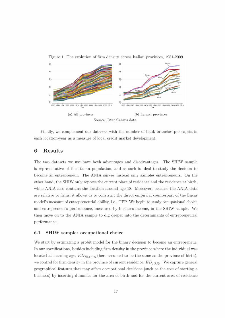
Figure 1: The evolution of firm density across Italian provinces, 1951-2009

.02

.04

.06

.08

.1.1

2

1950 1955 1960 1965 1970 1975 1980 1985 1990 1995 2000 2005 2010Year

(a) All provinces

Florence

Bologna

Milan

Venice

Palermo

Naples

Rome

Bari

Cagliari

Trieste

Genoa

Turin

.02

.04

.06

.08

.1.1

2

1950 1955 1960 1965 1970 1975 1980 1985 1990 1995 2000 2005 2010 2015Year

(b) Largest provinces

Source: Istat Census data

Finally, we complement our datasets with the number of bank branches per capita in

each location-year as a measure of local credit market development.

6 Results

The two datasets we use have both advantages and disadvantages. The SHIW sample

is representative of the Italian population, and as such is ideal to study the decision to

become an entrepreneur. The ANIA survey instead only samples entrepreneurs. On the

other hand, the SHIW only reports the current place of residence and the residence at birth,

while ANIA also contains the location around age 18. Moreover, because the ANIA data

are relative to firms, it allows us to construct the direct empirical counterpart of the Lucas

model’s measure of entrepreneurial ability, i.e., TFP. We begin to study occupational choice

and entrepreneur’s performance, measured by business income, in the SHIW sample. We

then move on to the ANIA sample to dig deeper into the determinants of entrepreneurial

performance.

6.1 SHIW sample: occupational choice

We start by estimating a probit model for the binary decision to become an entrepreneur.

In our specifications, besides including firm density in the province where the individual was

located at learning age, EDj(i,tL)tL(here assumed to be the same as the province of birth),

we control for firm density in the province of current residence, EDj(i,t)t. We capture general

geographical features that may affect occupational decisions (such as the cost of starting a

business) by inserting dummies for the area of birth and for the current area of residence

17

of the individual (either four macro area dummies - North-east, North-west, Center, South-

islands- or 20 regional dummies). In addition, we control for individual demographics such

as gender, age, educational attainment, work experience, a dummy if the parents were

entrepreneurs and family characteristics (whether married, number of earners, and family

size). A key issue in the choice to become an entrepreneur is access to finance. A large

literature argues that liquidity constraints and easiness in raising external capital foster

entrepreneurship (see e.g., Evans and Jovanovic, 1989; Banerjee and Newman, 1994). It

might be that firm density at learning age reflects local financial development as more

firms may be started where capital is easier to raise. To account for this we control for

the number of bank branches per capita in the province at learning age and for the same

variable in the province of residence at the time the survey was run. As shown by Guiso,

Sapienza, and Zingales (2004) the number of bank branches per capita predicts the easiness

in obtaining external finance. All regressions contain (unreported) dummies for education,

year, and sector. Given that our main variable of interest (ED at learning age) varies at the

province-year level, we cluster standard errors accordingly. Results are robust to alternative

clustering schemes.

Results are shown in Table 2 for the broader definition of entrepreneurship, which in-

cludes the self employed, partners of a company and owners that run an incorporated

business. Marginal effects are reported throughout. In column (1) we report the result

of a regression with ED at learning age without controlling for current ED . People who

grew up in provinces with a higher firm density are more likely to become entrepreneurs.

As for the other controls, bank branches per capita at learning age have no statistically

significant effect. Males are more likely to be entrepreneurs, as well as older and married

individuals. Having a parent that was an entrepreneur has a strong positive impact of being

an entrepreneur, consistent with most literature on the determinants of entrepreneurship.

Moreover, the number of income recipients within a household also exerts a positive effect,

arguably because employed family members are at time a source of startup capital and of

income insurance, important to smooth out entrepreneurial income fluctuations.

In column (2) we add current ED . This is a key control, given that, for stayers, current

and learning age ED are correlated, so that the latter might just be proxying for the former.

We also control for current bank branches per capita. As expected the coefficient on learning

age ED decreases, from 1.14 to 0.75, but remains large and statistically significant. Current

ED has a slightly larger coefficient (1.0) and is also significant.15 Increasing ED at learning

15It is worth stressing that while the correlation between the choice to become an entrepreneur and currentED may suffer from the reflection problem (Manski, 1994), our variable of interest - ED at learning age - is

18

age by one standard deviation increases the probability that an individual decides to become

an entrepreneur by 1.5 percentage points, 8% of the sample mean.

Having established this basic pattern, we now check whether it is robust to a number

of potential objections. As discussed in Section 4, there is still the possibility that our

results are driven by unobserved local factors that drive both ED at learning age and en-

trepreneurial outcomes later in life, such as school quality, genetic differences and differences

in culture. Regarding school quality, ideally one would like to control for it at the local

level at the time of learning. Unfortunately there is no source of information on school

quality at the local level over the required time span and thus we cannot control for this

potential confounding factor in the regressions. However, we do observe school quality in

recent years. If, as the objection holds, school quality is higher in high ED areas and this

leads to higher human capital (and thus better entrepreneurs), we should find a positive

correlation between school quality and ED even today (when we have standardized mea-

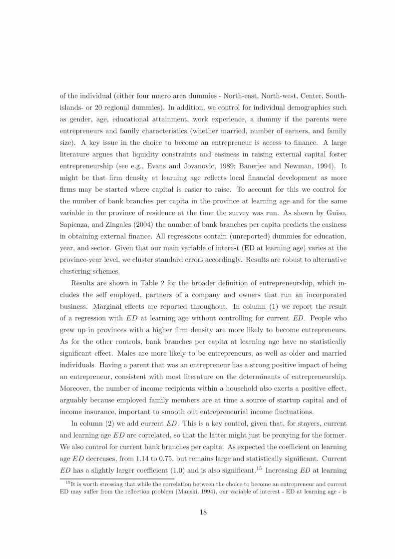
sures of students achievements). We use test scores in fifth grade and run a regression of

average test results at the province level on current ED, after controlling for macro area

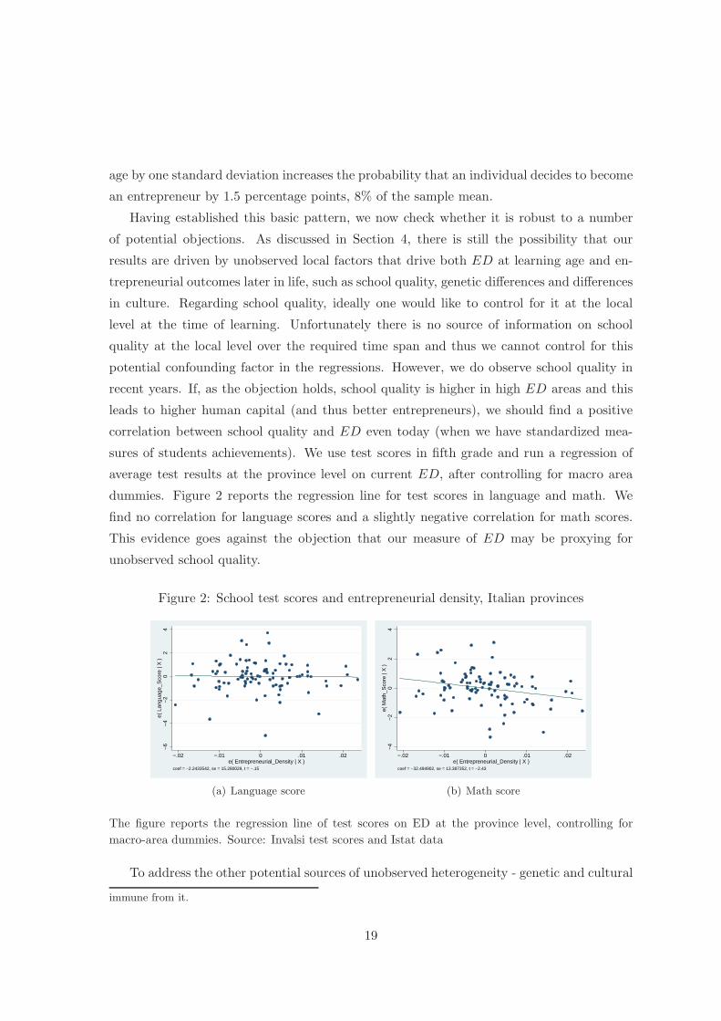
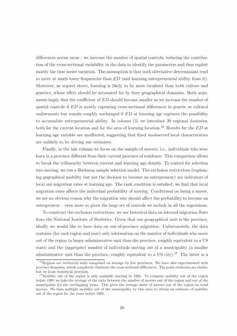
dummies. Figure 2 reports the regression line for test scores in language and math. We

find no correlation for language scores and a slightly negative correlation for math scores.

This evidence goes against the objection that our measure of ED may be proxying for

unobserved school quality.

Figure 2: School test scores and entrepreneurial density, Italian provinces

−6

−4

−2

02

4e(

Lan

guag

e_S

core

| X

)

−.02 −.01 0 .01 .02e( Entrepreneurial_Density | X )

coef = −2.2433542, se = 15.280029, t = −.15

(a) Language score

−4

−2

02

4e(

Mat

h_S

core

| X

)

−.02 −.01 0 .01 .02e( Entrepreneurial_Density | X )

coef = −32.494902, se = 13.387352, t = −2.43

(b) Math score

The figure reports the regression line of test scores on ED at the province level, controlling for

macro-area dummies. Source: Invalsi test scores and Istat data

To address the other potential sources of unobserved heterogeneity - genetic and cultural

immune from it.

19

differences across areas - we increase the number of spatial controls, reducing the contribu-

tion of the cross-sectional variability in the data to identify the parameters and thus exploit

mostly the time series variation. The assumption is that such alternative determinants tend

to move at much lower frequencies than ED (and learning entrepreneurial ability from it).

Moreover, as argued above, learning is likely to be more localized than both culture and

genetics, whose effect should be accounted for by finer geographical dummies. Both argu-

ments imply that the coefficient of ED should become smaller as we increase the number of

spatial controls if ED is mostly capturing cross sectional differences in genetic or cultural

endowments but remain roughly unchanged if ED at learning age captures the possibility

to accumulate entrepreneurial ability. In column (3) we introduce 20 regional dummies,

both for the current location and for the area of learning location.16 Results for the ED at

learning age variable are unaffected, suggesting that fixed unobserved local characteristics

are unlikely to be driving our estimates.

Finally, in the last column we focus on the sample of movers, i.e., individuals who were

born in a province different from their current province of residence. This comparison allows

to break the collinearity between current and learning age density. To control for selection

into moving, we run a Heckman sample selection model. The exclusion restrictions (explain-

ing gegraphical mobility but not the decision to become an entrepreneur) are indicators of

local out-migration rates at learning age. The rank condition is satisfied: we find that local

migration rates affects the individual probability of moving. Conditional on being a mover,

we see no obvious reason why the migration rate should affect the probability to become an

entrepreneur – even more so given the large set of controls we include in all the regressions.

To construct the exclusion restrictions, we use historical data on internal migration flows

from the National Institute of Statistics. Given that our geographical unit is the province,

ideally we would like to have data on out-of-province migration. Unfortunately, the data

contains (for each region and year) only information on the number of individuals who move

out of the region (a larger administrative unit than the province, roughly equivalent to a US

state) and the (aggregate) number of individuals moving out of a municipality (a smaller

administrative unit than the province, roughly equivalent to a US city).17 The latter is a

16Regions are territorial units comprised on average by five provinces. We have also experimented withprovince dummies, which completely eliminate the cross sectional differences. The point estimates are similarbut we loose statistical precision.

17Mobility out of the region is only available starting in 1995. To compute mobility out of the regionbefore 1995 we take the average of the ratio between the number of movers out of the region and out of themunicipality for the overlapping years. This gives the average share of movers out of the region on totalmovers. We then multiply mobility out of the municipality by this ratio to obtain an estimate of mobilityout of the region for the years before 1995.

20

combination of intra- and inter-regional mobility. Since provinces are closer to a region than

a municipality (there are 20 regions, 95 provinces, and 8,100 municipalities in Italy), we

focus on out-of-region migration rates, which we obtain by dividing the annual number of

out of the region migrants and the regional population. Given that we do not know the exact

year of the move (as we only know province of birth and the current province of residence),

we take the average mobility rate in the ten years before and ten years after learning age

and include them in the first stage of the Heckman procedure. We report the first stage in

the appendix. The mobility indicators are statistically significant. Since migration occurs

in waves, we find the intuitive result that the likelihood to move is higher if past migration

out of the region has been low or future mobility is higher. The results of the second stage

are reported in Column (4). The basic result is unchanged but the coefficient becomes

substantially larger, a pattern that will also emerge in the other regressions focusing on

movers.

Table 3 replicates the same regressions using the more stringent definition of entrepreneur-

ship which excludes self employment. This decreases the incidence of entrepreneurship from

19% to 8% (see Table 1). Results are qualitatively confirmed using this alternative defini-

tion. The point estimates are reduced by half (with the exception of the movers sample),

which is expected as the share of entrepreneurs is substantially smaller. According to the

estimates of column (2), increasing density at learning age by one standard deviation in-

creases the probability that an individual becomes an entrepreneur by 0.8 percentage points,

which represents a slightly larger increase relative to the sample mean than in the case of

definition I (10% versus 8%).

6.2 SHIW sample: performance

We next study entrepreneurs’ success, measured by income from business. Since this is

available only for entrepreneurs, we estimate a Heckman selection model to correct for

selection into entrepreneurship and use as an exclusion restriction the number of family

earners, which we assume affects the decision to become an entrepreneur (if other family

earners offer some earnings risk diversification) but not entrepreneurial success. Otherwise

the set of controls is the same as in the probit estimates in Tables 2 and 3. Results are

shown in Table 8 for the broad definition of entrepreneur. ED at learning age has a

positive and strongly significant effect on the (log of) entrepreneur’s earnings. The effect

is slightly smaller but retains fully its statistical significance even after controlling for the

current firms density in the province (column 2). The effect of current ED is positive and

21

significant, consistent with a large literature on agglomeration economies (Rosenthal and

Strange, 2004a; Moretti, 2011), but the effect of ED at learning age is almost twice as large

(5.4 vs. 3.2), and highly statistically significant. In terms of magnitude, the estimate implies

that increasing density at learning age by one standard deviation increases entrepreneurial

income by 11%.

According to these estimates, external effects related to firm density that take place

at learning age are more important for firm profits than current externalities. This is an

important result for the literature on agglomeration economies and the channels through

which they operate. Duranton and Puga (2004b) propose three channels through which

agglomeration economies can affect firm performance: the opportunities to learn from other

firms, the size of the local work force (which can increase the division of labor and the

quality of job-worker matches), and a greater variety of intermediate inputs. Of these three

channels, only learning can have effects that persist once an entrepreneur moves from a high

density area. Our results therefore indicate that learning externalities are at play in the

determination of agglomeration economies.18 Moreover, they also point to a specific channel

of learning externalities, that is, those that get embedded in the individual’s human capital

in the coming of age years, which are distinct from contemporaneous knowledge spillovers

that result from being located in a certain area in the current period.

As for the effect of other controls, we find that male entrepreneurs earn a substantial

premium (more than 40%) over female entrepreneurs. Older entrepreneurs earn more, as

well as those with a parent that was already an entrepreneur19 and who are married.

In column (3) we include regional dummies (both for current and learning age location)

and find no differences in the estimates, in line with the hypothesis that the ED at learning

age is not proxying for other unobservables that determine both ED at learning age and

entrepreneurial success today.

In the last column we focus on the sample of movers, where identification is robust to the

concerns discussed in Section 4. Column (4) corrects for joint selection into entrepreneurship

as well as moving, where the instruments for mobility are the same as in the occupational

choice regressions of the previous tables. We find that the basic conclusions are confirmed,

with the effect becoming slightly larger compared to the whole sample.

18Of course, this does not imply that the other sources of externalities are absent. In fact, ED is a naturalindicator of learning externalities, but not necessarily of the size of the local workforce or of intermediateinput varieties, typically captured by other indicators (Glaeser et al., 1992).

19Growing up in an entrepreneurial family can be an important alternative source of learning. Of course,this cannot be told apart from genetic effects, so that one cannot interpret this coefficient planing as evidencefor learning.

22

Table 5 replicates the estimate using the stricter definition of entrepreneurship. This

reduces the observations from 11,498 to 5,083. The reduction in the sample size reduces

the statistical power so that, in the specification with regional dummies, we loose signifi-

cance. However, the pattern that emerges is fully consistent with that based on the broader

definition of entrepreneurship. We also find that in the movers sample the coefficient is

substantially larger than in the overall sample, arguably because breaking the correlation

between ED at learning age and current ED is more important in the smaller sample of

strictly defined entrepreneurs.

6.3 ANIA sample: performance

To further investigate the effects of ED on entrepreneurial quality, we now turn to the ANIA

sample. We use the same framework as in the SHIW sample, with a few exceptions. First, we

only study entrepreneurial success, as this is a sample of entrepreneurs and therefore cannot

be used to study occupational choice. Following Lucas (1978), we measure entrepreneurial

quality with firm TFP. Second, we measure ED in the location in which the entrepreneur

was actually living at age 18, rather than at birth. This is indeed important, as the two

locations differ for about 15% of cases in our sample. Third, the set of controls is the same

as in the SHIW regressions, with the exception that experience is defined in terms of years

since the individual started managing the firm, an information not avaliable in the SHIW

and that could have an independent effect of performance. As before, we cluster standard

errors at learning age-LSS level and, as before, results are robust to alternative clustering

schemes.

Table 6 shows the results. ED at learning age has a positive and precisely estimated

effect on the firm TFP (column 1). Increasing ED at learning age by one standard devia-

tion (0.02) increases TFP by 8.6%. None of the other controls display a significant effect,

arguably due to the fact that we have a much smaller sample compared to the SHIW one.

It is theorefore remarkable that ED at learning age is statistically significant also in this

dataset. In column (2) we add current ED, finding a positive but statistically insignificant

estimate. The coefficient on ED at learning age increases slightly (to about 5) and remains

statistically significant at the 5% level. As in the SHIW data, therefore, we find the striking

result that learning age externalities play a stronger role than current production external-

ities. We also notice that the elasticity of entrepreneurial quality to ED is very close in

the two datasets, although the sample and the variables used to measure entrepreneurial

quality are different.

23

The remaining columns perform a series of robustness checks. First, we control for ED

at birth (column 3). A growing literature stresses the role of early education on professional

outcomes (Heckman, Pinto, and Savelyev, 2013). Extrapolating from this literature it may

be argued that the economic environment that matters most to accumulate entrepreneurial

ability is the one in the early years of development. In the ANIA sample we have direct

information on place of residence both at birth and at 18. For movers, this breaks the

strong correlation in ED at birth and at learning age that results from assuming that the

two locations are the same, as we are forced to do in the SHIW sample. The estimated

coefficient of ED at birth is not statistically different from zero, while that of ED at learn-

ing age is unaffected, supporting the idea that learning entrepreneurial talents from other

entrepreneurs occurs in the early years or just before the beginning of one’s professional life.

This result also allows us to address a potential competing explanation: genetic differences.

In fact, the birthplace should be a better identifier of genetic influences than the place where

one grows up. The significance of ED at learning age and the lack of significance of ED

at birth allow us to reject the hypothesis that higher entrepreneurial density proxies for

genetic propensity to engage in entrepreneurship.

These findings could still be consistent with a cultural explanation if the culture that

matters for entrepreneurship is not acquired in the early years of life but only later. If

the density where one grows up is a reflection of an underlying entrepreneurial culture, our

measure might just be proxying for it rather than for learning opportunities. To address

this, we rely on the idea that culture evolves slowly and the geographical unit that is covered

by a culture is broader than that where learning entrepreneurial abilities from firms takes

place. Accordingly, in column (4) we expand the number of spatial controls to account for

potential spatially correlated effects. Given that the geographical unit for ED is the LLS,

we can use finer controls than those of the SHIW sample and insert 95 province dummies

(rather than 20 regional dummies). Since provincial governments are in charge of managing

schools, provincial dummies also account for any persistent geographical differences in the

quality of schooling. As before, we use separate dummies for location at learning age and

current location. Again, we find that the point estimates are unchanged – if anything, they

become larger – and that the coefficient is statistically significant at the 5% level.20

Finally, we focus on the the sample of movers employing a Heckman sample selection

20We have also experimented with dummies at the LLS level, thus exploiting for identification of learningeffects only on the time variation in ED. As with the SHIW data, estimates for the effect of ED at learningage are similar in magnitude but with larger standard errors. This is not surprising, given the large numberof dummies (more than 400) and the limited sample size.

24

model. Compared to the SHIW regressions, we introduce two slight modifications given

that we have richer data. First, we use the mobility rate out of the municipality rather

than out the region. In fact, a LLS contains on average 10 municipalities while regions

contain on average around 40 LLS. Mobility out of the municipality is therefore a closer

proxy to mobility out of the LLS than mobility out of the region. Second, we only use the

average mobility rate in the 10 years after learning age. Differently from the SHIW sample

(where we observe the province of birth but not the province of residence at learning age),

in the ANIA data we know that the individual was still resident in the LLS of learning at

18, so we can disregard prior mobility. The first stage, reported in the appendix, shows

that the instrument has the expected positive sign and is statistically significant. Column

(5) shows that, as in the SHIW sample, the effect of ED at learning age becomes stronger

and more precisely estimated.

As a final check, we have used sales per worker to measure entrepreneurial quality.

While TFP is the closest empirical counterpart to ability in the Lucas model, estimating

TFP requires more assumptions than just computing a simple measure of labor productivity.

Results in Table 7 confirm all those obtained with TFP. The coefficient on ED at learning

age tends to be larger and more precisely estimated. Increasing density at learning age by

one standard deviation results in an increase in sales per worker of around 22%. A possible

explanation is that growing up in denser areas not only improves ability, but it also leads

entrepreneurs to increase the capital-labor and intermediate inputs-labor ratio, leading to

an even stronger effect on labor productivity.

Overall, we take this evidence as supportive of the idea that one important channel

through which individuals acquire entrepreneurial abilities is early exposure to a richer

entrepreneurial environment.

7 What features of entrepreneurship are learnable?

Being an entrepreneur requires multiple talents. The entrepreneur develops new ideas,

evaluates their market appeal, organizes production, bears the risk of failure. Sorensen

and Chang (2008) argue that entrepreneurship is defined by three features: risk bearing,

propensity to innovate, and coordination ability. These three features are well rooted in the

economics tradition. The role of the entrepreneur as the bearer of risk dates back to Knight

(1921), who ascribes the very existence of the firm to its role as an insurance provider.

Schumpeter (1911) emphasized the role of the entrepreneur as the carrier of innovation

and creative destruction deriving from innovation as the key source of growth in market

25

economies. But in addition to a propensity to innovate and to bear the risk of such a

process, the entrepreneur also needs to be able to implement an idea, organize production,

and bring the product to the market. Marshall (1890) was the first to stress the importance

of localized spillovers to learn “the mysteries of the trade”.

In this section we offer empirical evidence on how “learnable” these three features are, us-

ing information from the ANIA survey. In the face-to-face interview respondents were asked

a set of questions aimed at eliciting risk preferences and identifying personality traits. We

briefly describe them here and report the full questions in the Appendix. First, respondents

were asked to choose between different investment strategies with decreasing risk-returns

profiles, ranked from 1 (high risk and high return) to 5 (low risk and low return). We use

the answers to this question as a measure of risk aversion. Second, the respondent was

asked to express, on a scale from 1 to 5, their preferences regarding drawing a ball from an

urn with 50 green and 50 yellow balls vs. drawing it from an urn containing an unknown

share of balls of each color. We use this question to measure ambiguity aversion. A mea-

sure of self-confidence was obtained by asking the entrepreneur whether she ranked herself

below, at the same level or above the average ability or other entrepreneurs. Optimism

is measured by the answer (on a scale from 0 to 10) to how much the respondent agrees

with the statement “All things considered I expect more good than bad things in life”. Job

satisfaction was measured from the answer to the question: “Excluding the monetary as-

pects and considering only the other characteristics of your job, can you tell me if they give

you more satisfaction or annoyance?”, again on a scale 0-10. Summary statistics for these

variables are reported in Table 8, Panel A.

The entrepreneur’s propensity to innovate is measured by two (arguably imperfect)

proxies. The first is the share of 2007 sales due to innovative or significantly improved

products or services that were introduced in the market in the 2005-2007 period. The second

is a score of the practices used by the firm to manage the innovation process, collected in the

managerial practices follow up survey described below. Descriptive statistics for all these

variables are in Table 8, Panel B.

The original survey lacks information on the ability to coordinate production or manage

the firm. In the Fall of 2012 we re-contacted the entrepreneurs in the ANIA sample and asked

them to participate in a second round of interviews to assess their managerial practices. We

used the methodology developed by the World Management Survey (WMS, see Bloom and

Van Reenen (2010a,b)). The WMS is based on a telephone double-blind survey technique

and comprises a set of open-ended questions, whose qualitative answers are then recoded

26

into quantitative measures with a score ranging between 1 (worst) to 5 (best managerial

practices). The questionnaire comprises five sections that consider different key areas of

management practices. We investigate three areas. The first section is Monitoring and

focuses on the monitoring of performance and reviewing the results. The second section is

Targets and aims at assessing the respondents’ managerial ability to identify quantitative

and qualitative targets, their interconnection and their temporal cascade. The third section

is People and it is concerned with human resource management, ranging from promoting

and rewarding employees based on performance, removing poor performers, and hiring and

retaining the best workers. The average score of the three areas defines the index of overall

managerial ability.21 Of the original 966 entrepreneurs, we were able to re-interview 388

(details on the data collection methodology are in the appendix, section A.2). Descriptive

statistics are in Table 8, Panel C.

As a first check, in Appendix Table A.3 we regress TFP on personality traits. We

have no a priori on how the degree of risk aversion or optimism should correlate with firm

level TFP. Indeed, the correlation is always insignificant. Next, we check if these traits are

correlated with ED at learning age. Given that what we are trying to measure is more

elusive than occupational choice or performance, and that the number of observations is

smaller, as we only use the cross section rather than the three years of data as with TFP, for

all regressions in this section we start with a parsimonious specification which only includes

macro area and sector dummies, and then add the individual controls. The results are

reported in Table 9. In general, we find no evidence that entrepreneurial traits are affected

by ED at learning age. Growing up in areas with greater firm density seems to lead to

higher risk aversion in the specification with individual controls (column 2), but precision

is low and the estimate changes sign and is not statistically significant controlling only for

sector and area dummies (column 1). Moreover, one would expect that ED at learning

age reduces risk aversion, as risk tolerance is one of the key features of entrepreneurship.

This evidence instead is consistent with the predominant role of the innate component in

explaining individual risk preferences found by Cesarini et al. (2009) using twin studies. All

other traits appear uncorrelated with ED at learning age. Overall, these results suggests

that traits are not affected by the entrepreneurial context at learning age, arguably because

a large component is genetically determined or acquired much earlier, perhaps within the

21The original WMS contains two additional areas, operations and leadership. These areas investigatepractices that are very sector specific, such as the operation of the production unit. Given that we have firmsfrom both manufacturing and services, we only investigated areas where practices are sufficiently similar toallow for the use of the same scheme of interview. In any case, in all regressions we use sector dummies.

27

family or at school (Heckman, Pinto, and Savelyev, 2013).

Next, we run the same exercise for innovation capacity. Table A.3 (column 6) and A.4

(column 5) in the Appendix show that the two measures of innovation are not correlated

with TFP. Consistently, we find no effect of ED at learning age on innovation capacity

(Table 10): the Schumpeterian component of entrepreneurship appears unrelated to ED at

learning age. This is indeed in line with Schumpeter’s original notion of the innovator as

the one that challenges established knowledge with new, unforeseen ideas – something that

is unlikely to be learned from others.

The ability to manage, however, is more likely to be learnable. Indeed, managerial

skills are precisely what one learns in business schools and colleges specialized in teaching

entrepreneurship. But these skills may possibly be learned also before college by direct

observation and exposure to adopted practices by the firms in the place where one grows

up.

We test this potential channel using the measures of managerial practices discussed

above. To first validate these measures, in Table A.4 we report the results of regressions

in which productivity and firm size (measured by the log of the number of employees) are

regressed on the managerial practices scores. As shown by Bloom and Van Reenen (2007)

and Bloom, Sadun, and Van Reenen (2012), managerial practices are strongly correlated

with the size of the firm and its productivity. This holds in our sample too: each type of

managerial practice, as well as the general index, is positively and significantly correlated

with TFP and firm size. Table 11 runs regressions of these measures on ED at learning age

controlling for current density. Interestingly, in the parsimonious specifications in which we

control only for current density and area and sector dummies, density at learning age has

a positive and statistically significant correlation with managerial practices, while current

density has a small and insignificant effect (columns 1, 3, and 5). The exception is People,

where the ED at learning age coefficient has a p-value of 11 percent. When we introduce

the individual controls, the effect of density at learning age retains its positive effect but its

size halves on average and the estimate looses precision, so that none of the coefficient is

statistically significant. This is most likely a reflection of the fact that measuring managerial

practices is a difficult task and that we have a limited number of observations (less than 400),

reducing statistical power. It turns out that the loss of significance of ED learn in Table 11 is

due to the inclusion of the age and experience variables. These variables are mechanically

correlated with ED at learning age, since the latter has a time varying component that

trends similarly to age and experience. The limited statistical power prevents us from

28

identifying separately the two effects.

There is also another, more economic reason that might explain the difficulty in singling

out the aspects of entrepreneurship that can be learned. Lazear (2005) argues that an

entrepreneur is a “Jack-of-all-trades”, i.e., an individual with a balanced set of skills, rather

than one that excels in any particular activity. Using data on Stanford GSB MBAs, he

finds that those who tend to perform uniformly well in (but not necessarily at the top

of) all courses are indeed more likely to become entrepreneurs than those who excel in

specific subjects. Similar conclusions are reached by Bruhn, Karlan, and Schoar (2013) in

their randomized trial in which managerial consulting services are provided to 150 SMEs in

Mexico. They find that managerial consulting does improve overall firm performance, but

no single aspect of managerial practices emerges as a key for the improvement. Profits and

TFP are comprehensive measures of entrepreneurial capability and clearly correlate with

learning opportunities. Singling out specific aspects, such as traits or particular managerial

capabilities, might instead be more difficult, as there is no single component that by itself

can explain entrepreneurial ability. This confirms the elusive nature of what makes a good

entrepreneur.

Overall, we take this evidence as suggesting that managerial capabilities can be learned

from other entrepreneurs, while both traits and innovation capacity might be more innate

components that are less subject to the influence of the economic environment.

8 Conclusions

This paper analyzes the extent to which growing up in a high entrepreneurial area increases

both the likelihood that an individual becomes an entrepreneur and her entrepreneurial

ability or success. We find evidence that this is indeed the case, as would be implied

by models where entrepreneurial ability is socially acquired. Interestingly, the effects of

entrepreneurial density at learning age are stronger than those of current entrepreneurial

density, which captures more traditional spillover effects. A remarkable finding is that the

results we find hold in two distinct datasets and are robust to a large set of controls. More-

over, we find suggestive evidence that individuals growing up in high firm density areas

acquire managerial skills, but that individual traits reflecting risk aversion, aversion to am-

biguity, self-confidence or optimism, and propensity to innovate (which are traditionally

associated to entrepreneurship) are independent of location. This suggests that the “per-

sonality traits” factor of entrepreneurship has a larger innate component, swamping any

effect played by the environment.

29

References

Banerjee, A.V. and A. Newman. 1994. “Poverty, Incentives and Development.” American

Economic Review Papers and Proceedings 84:211–215.

Barlow, R.E. and F. Proschan. 1975. Statistical Theory of Reliability and Life Testing. Holt,

Rinehart and Winston, New York.

Bisin, Alberto and Thierry Verdier. 2001. “The economics of cultural transmission and the

dynamics of preferences.” Journal of Economic Theory 97:298–319.

Bloom, Nicholas, Christos Genakos, Raffaella Sadun, and John Van Reenen. 2012. “Man-

agement practices across firms and countries.” The Academy of Management Perspectives

26:12–33.

Bloom, Nicholas and John Van Reenen. 2007. “Measuring and Explaining Manage-

ment Practices Across Firms and Countries.” The Quarterly Journal of Economics

122 (4):1351–1408.

———. 2010a. “New Approaches to Surveying Organizations.” American Economic Review

100 (2):105–09.

———. 2010b. “Why Do Management Practices Differ across Firms and Countries?” Jour-

nal of Economic Perspectives 24 (1):203–24.

Bloom, Nick, Raffaella Sadun, and John Van Reenen. 2012. “Americans do I.T. Better: US

Multinationals and the Productivity Miracle.” American Economic Review 102:167–201.

Bruhn, Miriam, Dean Karlan, and Antoinette Schoar. 2013. “The Impact of Consulting Ser-

vices on Small and Medium Enterprises: Evidence from a Randomized Trial in Mexico.”

Mimeo, MIT Sloan.

Cavalli Sforza, Luigi and Walter F. Bodmer. 1971. The genetics of human population. W.

H. Freeman and C., San Francisco.

Cesarini, David, Christopher T Dawes, Magnus Johannesson, Paul Lichtenstein, and Bjorn

Wallace. 2009. “Genetic variation in preferences for giving and risk taking.” The Quarterly

Journal of Economics 124:809–842.

Chetty, Raj and Nathaniel Hendren. 2015. “The Impacts of Neighborhoods on Intergen-

erational Mobility: Childhood Exposure Effects and County-Level Estimates.” Mimeo,

Harvard University.

Chinitz, Benjamin. 1961. “Contrasts in agglomeration: New York and Pittsburgh.” The

American Economic Review 51:279–289.

30

Cingano, Federico and Fabiano Schivardi. 2004. “Identifying the sources of local productiv-

ity growth.” Journal of the European Economic Association 2 (June):720–742.

De Figueiredo, Rui J.P., Philipp Meyer-Doyle, and Evan Rawley. 2013. “Inherited agglom-

eration effects in hedge fund spawns.” Strategic Management Journal 34 (7):843–862.

De la Roca, Jorge and Diego Puga. 2013. “Learning by working in big cities.” Mimeo,

CEMFI.

Dohmen, Thomas, Armin Falk, David Huffman, and Uwe Sunde. 2012. “The intergen-

erational transmission of risk and trust attitudes.” The Review of Economic Studies

79:645–677.

Duranton, G. and D. Puga. 2004a. “Micro-foundations of urban agglomeration economies.”

In Handbook of Regional and Urban Economics, vol. 4, edited by V. Henderson and J.F.

Thisse. Amsterdam: North Holland.

Duranton, Gilles and Diego Puga. 2004b. “Micro-foundations of urban agglomeration

economies.” Elsevier, 2063–2117.

Erikson, Erik H. 1968. Identity, Youth and Crisis. New York: WW Norton.

Evans, David S. and Boyan Jovanovic. 1989. “An Estimated Model of Entrepreneurial

Choice under Liquidity Constraints.” Journal of Political Economy 97:808–827.

Giannetti, Mariassunta and Andrei Simonov. 2009. “Social interactions and entrepreneurial

activity.” Journal of Economics & Management Strategy 18:665–709.

Glaeser, E. L., H. D. Kallal, J. A. Scheinkman, and A. Shleifer. 1992. “Growth in Cities.”

Journal of Political Economy 100:1125–1152.

Glaeser, E.L., W.R. Kerr, and G.A.M. Ponzetto. 2010. “Clusters of entrepreneurship.”

Journal of Urban Economics 67:150–168.

Glaeser, E.L. and D.C. Mare. 2001. “Cities and Skills.” Journal of Labor Economics

19:316–342.

Guiso, L., P. Sapienza, and L. Zingales. 2004. “Does Local Financial Development Matter?”

The Quarterly Journal of Economics 119:929–969.

Guiso, Luigi and Fabiano Schivardi. 2011. “What determines entrepreneurial clusters?”

Journal of the European Economic Association 9:61–86.

Harris, Judith Rich. 2011. The nurture assumption: Why children turn out the way they

do. Free Press.

31

Heckman, J., R. Pinto, and P. Savelyev. 2013. “Understanding the mechanisms through

which an influential early childhood program boosted adult outcomes.” American Eco-

nomic Review 103:2052–2086.

Hoang, Ha and Bostjan Antoncic. 2003. “Network-based research in entrepreneurship: A

critical review.” Journal of business venturing 18 (2):165–187.

Hurrelmann, Klaus. 1988. Social structure and personality development: The individual as

a productive processor of reality. Cambridge: Cambridge University Press.

Kihlstrom, Richard and Jean-Jacques Laffont. 1979. “A General Equilibrium Theory of

Firm Formation Based on Risk Aversion.” Journal of Political Economy 87:719–48.

Knight, Frank H. 1921. Risk, Uncertainty and Profit. Houghton Miffin, New York.

Lazear, E. P. 2005. “Entrepreneurship.” Journal of Labor Economics 23:649–680.

Lindquist, Matthew J, Joeri Sol, and Mirjam Van Praag. 2015. “Why Do Entrepreneurial

Parents Have Entrepreneurial Children?” Journal of Labor Economics 33:269–296.

Lucas, Robert E., Jr. 1978. “On the Size Distribution of Business Firms.” Bell Journal of

Economics 2:508–523.

Manski, C. 1994. “Identification of Endogenous Social Effects: the Reflection Problem.”

Review of Economic Studies 60:531–542.

Marshall, A. 1890. Principles of Economics. London:Macmillan.

Matano, Alessia and Paolo Naticchioni. 2012. “What drives the urban wage premium?

evidence along the wage distribution.” Tech. rep. Mimeo, Sapienza University of Rome.

Michelacci, Claudio and Olmo Silva. 2007. “Why so many local entrepreneurs?” The

Review of Economics and Statistics 89 (4):615–633.

Moretti, E. 2011. “Local labor markets.” In Handbook of labor economics, vol. 4, edited by

D. Card and O. Ashenfelter. Elsevier, 1237–1313.

Nicolaou, N. and S. Shane. 2010. “Entrepreneurship and occupational choice: Genetic and

environmental influences.” Journal of Economic Behavior & Organization 76:3–14.

Nicolaou, N., S. Shane, L. Cherkas, J. Hunkin, and T.D. Spector. 2008. “Is the tendency

to engage in entrepreneurship genetic?” Management Science 54:167–179.

Parker, Simon C. 2009. The economics of entrepreneurship. Cambridge University Press.

Rosen, Sherwin. 1982. “Authority, control, and the distribution of earnings.” The Bell

Journal of Economics :311–323.

32

Rosenthal, S. and W. Strange. 2004a. “Evidence on the Nature and Sources of Agglom-

eration Economies.” In Handbook of Regional and Urban Economics, vol. 4, edited by

V. Henderson and J.F. Thisse. Amsterdam: North Holland.

Rosenthal, Stuart S and William C Strange. 2004b. “Evidence on the nature and sources

of agglomeration economies.” Handbook of regional and urban economics 4:2119–2171.

Sacerdote, Bruce. 2011. “Nature and nurture effects on childrens outcomes: What have we

learned from studies of twins and adoptees.” In Handbook of social economics, Volume

1A, vol. 1, edited by Jess Benhabib, Alberto Bisin, and Matthew O Jackson. 1–30.

Schumpeter, Joseph. 1911. The Theory of Economic Development. Harvard University

Press, Cambridge, Mass.

Sorensen, J. and P. Chang. 2008. “Determinants of successful entrepreneurship: A review

of the recent literature.” Report for the Ewing Marion Kauffman Foundation.

Wahba, Jackline and Yves Zenou. 2012. “Out of Sight, out of mind: Migration, en-

trepreneurship and social capital.” Regional Science and Urban Economics 42 (5):890–

903.

Williamson, Oliver E. 2000. “The new institutional economics: taking stock, looking ahead.”

Journal of economic literature :595–613.

Zhang, Z., M.J. Zyphur, J. Narayanan, R.D. Arvey, S. Chaturvedi, B.J. Avolio, P. Lichten-

stein, and G. Larsson. 2009. “The genetic basis of entrepreneurship: Effects of gender and

personality.” Organizational Behavior and Human Decision Processes 110 (2):93–107.

33

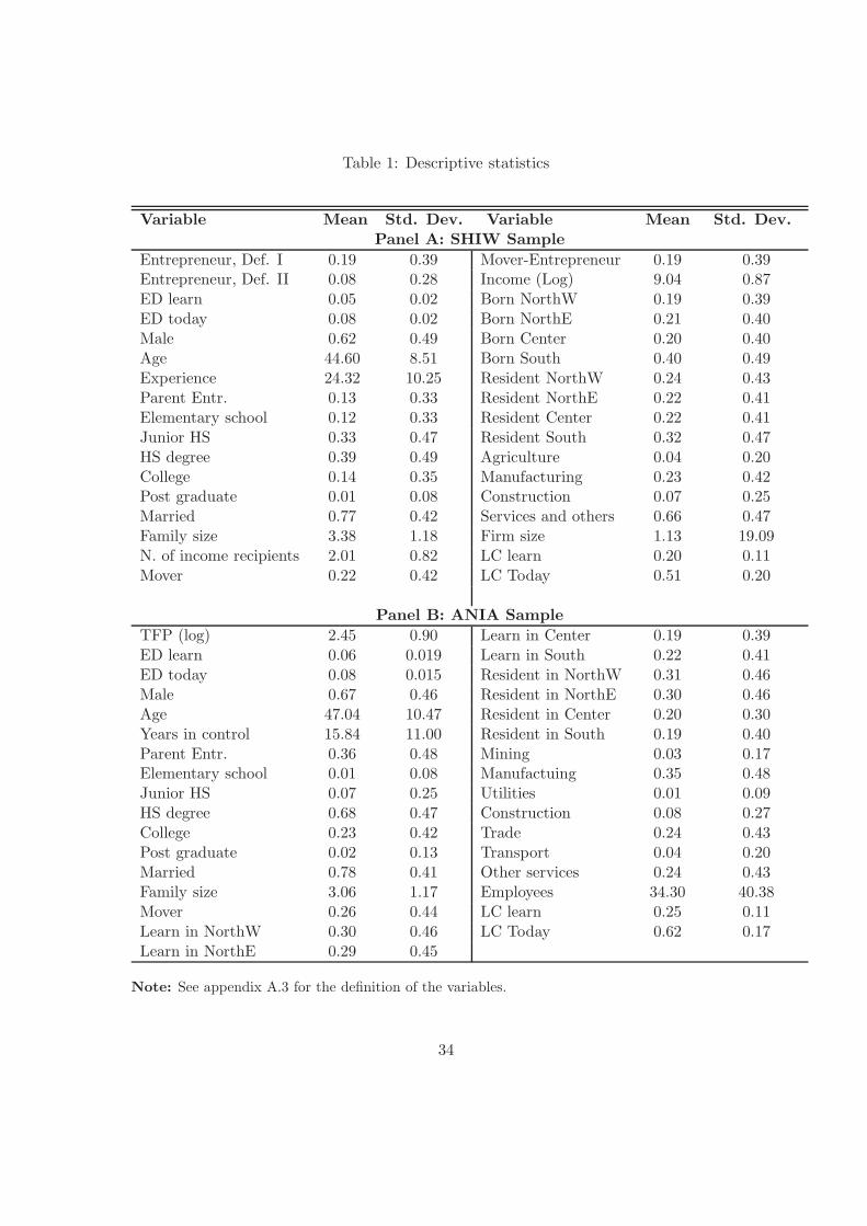
Table 1: Descriptive statistics

Variable Mean Std. Dev. Variable Mean Std. Dev.

Panel A: SHIW Sample

Entrepreneur, Def. I 0.19 0.39 Mover-Entrepreneur 0.19 0.39Entrepreneur, Def. II 0.08 0.28 Income (Log) 9.04 0.87ED learn 0.05 0.02 Born NorthW 0.19 0.39ED today 0.08 0.02 Born NorthE 0.21 0.40Male 0.62 0.49 Born Center 0.20 0.40Age 44.60 8.51 Born South 0.40 0.49Experience 24.32 10.25 Resident NorthW 0.24 0.43Parent Entr. 0.13 0.33 Resident NorthE 0.22 0.41Elementary school 0.12 0.33 Resident Center 0.22 0.41Junior HS 0.33 0.47 Resident South 0.32 0.47HS degree 0.39 0.49 Agriculture 0.04 0.20College 0.14 0.35 Manufacturing 0.23 0.42Post graduate 0.01 0.08 Construction 0.07 0.25Married 0.77 0.42 Services and others 0.66 0.47Family size 3.38 1.18 Firm size 1.13 19.09N. of income recipients 2.01 0.82 LC learn 0.20 0.11Mover 0.22 0.42 LC Today 0.51 0.20

Panel B: ANIA Sample

TFP (log) 2.45 0.90 Learn in Center 0.19 0.39ED learn 0.06 0.019 Learn in South 0.22 0.41ED today 0.08 0.015 Resident in NorthW 0.31 0.46Male 0.67 0.46 Resident in NorthE 0.30 0.46Age 47.04 10.47 Resident in Center 0.20 0.30Years in control 15.84 11.00 Resident in South 0.19 0.40Parent Entr. 0.36 0.48 Mining 0.03 0.17Elementary school 0.01 0.08 Manufactuing 0.35 0.48Junior HS 0.07 0.25 Utilities 0.01 0.09HS degree 0.68 0.47 Construction 0.08 0.27College 0.23 0.42 Trade 0.24 0.43Post graduate 0.02 0.13 Transport 0.04 0.20Married 0.78 0.41 Other services 0.24 0.43Family size 3.06 1.17 Employees 34.30 40.38Mover 0.26 0.44 LC learn 0.25 0.11Learn in NorthW 0.30 0.46 LC Today 0.62 0.17Learn in NorthE 0.29 0.45

Note: See appendix A.3 for the definition of the variables.

34

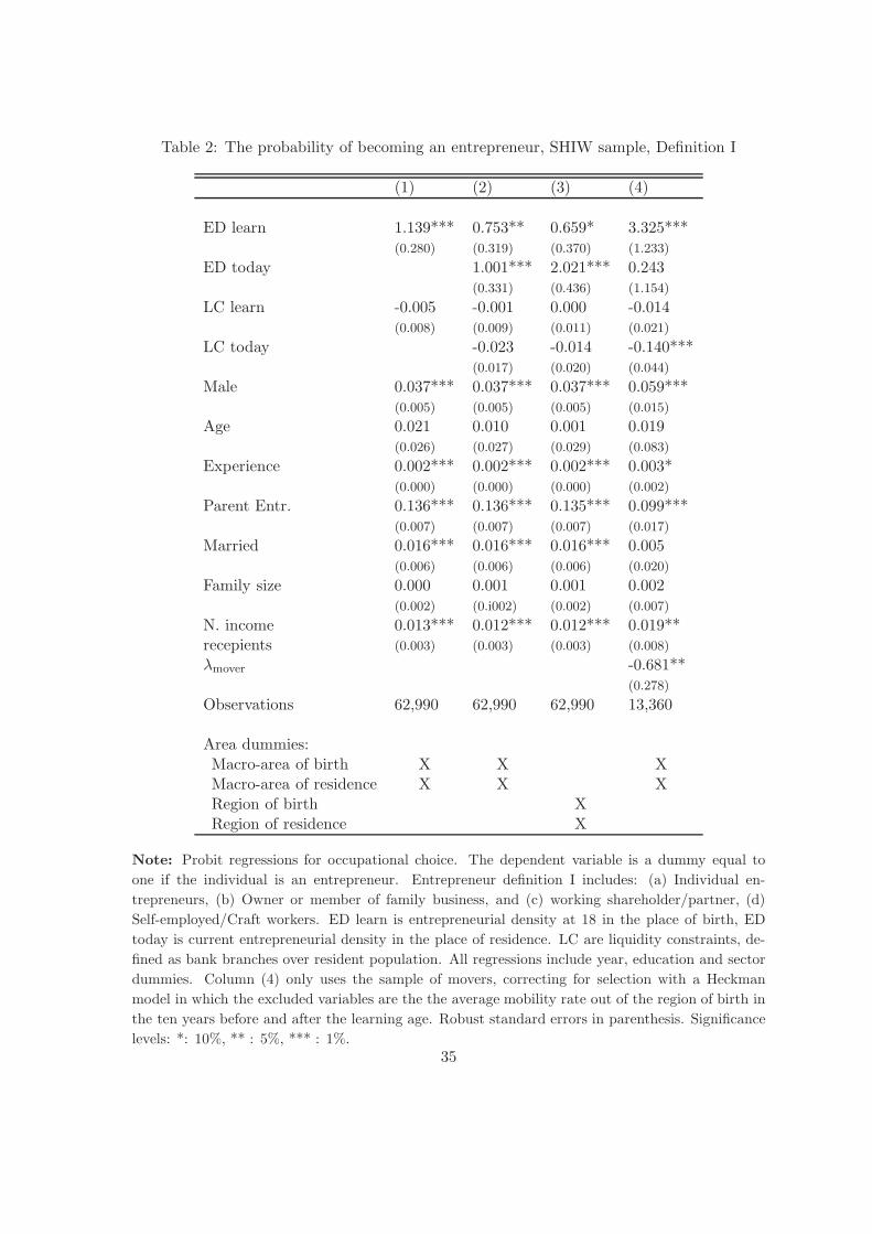
Table 2: The probability of becoming an entrepreneur, SHIW sample, Definition I

(1) (2) (3) (4)

ED learn 1.139*** 0.753** 0.659* 3.325***(0.280) (0.319) (0.370) (1.233)

ED today 1.001*** 2.021*** 0.243(0.331) (0.436) (1.154)

LC learn -0.005 -0.001 0.000 -0.014(0.008) (0.009) (0.011) (0.021)

LC today -0.023 -0.014 -0.140***(0.017) (0.020) (0.044)

Male 0.037*** 0.037*** 0.037*** 0.059***(0.005) (0.005) (0.005) (0.015)

Age 0.021 0.010 0.001 0.019(0.026) (0.027) (0.029) (0.083)

Experience 0.002*** 0.002*** 0.002*** 0.003*(0.000) (0.000) (0.000) (0.002)

Parent Entr. 0.136*** 0.136*** 0.135*** 0.099***(0.007) (0.007) (0.007) (0.017)

Married 0.016*** 0.016*** 0.016*** 0.005(0.006) (0.006) (0.006) (0.020)

Family size 0.000 0.001 0.001 0.002(0.002) (0.i002) (0.002) (0.007)

N. income 0.013*** 0.012*** 0.012*** 0.019**recepients (0.003) (0.003) (0.003) (0.008)

λmover -0.681**(0.278)

Observations 62,990 62,990 62,990 13,360

Area dummies:Macro-area of birth X X XMacro-area of residence X X XRegion of birth XRegion of residence X

Note: Probit regressions for occupational choice. The dependent variable is a dummy equal to

one if the individual is an entrepreneur. Entrepreneur definition I includes: (a) Individual en-

trepreneurs, (b) Owner or member of family business, and (c) working shareholder/partner, (d)

Self-employed/Craft workers. ED learn is entrepreneurial density at 18 in the place of birth, ED

today is current entrepreneurial density in the place of residence. LC are liquidity constraints, de-

fined as bank branches over resident population. All regressions include year, education and sector

dummies. Column (4) only uses the sample of movers, correcting for selection with a Heckman

model in which the excluded variables are the the average mobility rate out of the region of birth in

the ten years before and after the learning age. Robust standard errors in parenthesis. Significance

levels: *: 10%, ** : 5%, *** : 1%.

35

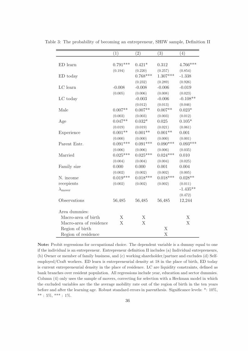
Table 3: The probability of becoming an entrepreneur, SHIW sample, Definition II

(1) (2) (3) (4)

ED learn 0.791*** 0.421* 0.312 4.766***(0.194) (0.220) (0.257) (0.854)

ED today 0.768*** 1.307*** -1.338(0.232) (0.289) (0.926)

LC learn -0.008 -0.008 -0.006 -0.019(0.005) (0.006) (0.008) (0.023)

LC today -0.003 -0.006 -0.108**(0.012) (0.013) (0.046)

Male 0.007** 0.007** 0.007** 0.023*(0.003) (0.003) (0.003) (0.012)

Age 0.047** 0.032* 0.025 0.105*(0.019) (0.019) (0.021) (0.061)

Experience 0.001** 0.001** 0.001** 0.001(0.000) (0.000) (0.000) (0.001)

Parent Entr. 0.091*** 0.091*** 0.090*** 0.093***(0.006) (0.006) (0.006) (0.035)

Married 0.025*** 0.025*** 0.024*** 0.010(0.004) (0.004) (0.004) (0.025)

Family size 0.000 0.000 0.001 0.004(0.002) (0.002) (0.002) (0.005)

N. income 0.019*** 0.018*** 0.018*** 0.028**recepients (0.002) (0.002) (0.002) (0.011)

λmover -1.435**(0.472)

Observations 56,485 56,485 56,485 12,244

Area dummies:Macro-area of birth X X XMacro-area of residence X X XRegion of birth XRegion of residence X

Note: Probit regressions for occupational choice. The dependent variable is a dummy equal to one

if the individual is an entrepreneur. Entrepreneur definition II includes (a) Individual entrepreneurs,

(b) Owner or member of family business, and (c) working shareholder/partner and excludes (d) Self-

employed/Craft workers. ED learn is entrepreneurial density at 18 in the place of birth, ED today

is current entrepreneurial density in the place of residence. LC are liquidity constraints, defined as

bank branches over resident population. All regressions include year, education and sector dummies.

Column (4) only uses the sample of movers, correcting for selection with a Heckman model in which

the excluded variables are the the average mobility rate out of the region of birth in the ten years

before and after the learning age. Robust standard errors in parenthesis. Significance levels: *: 10%,

** : 5%, *** : 1%.

36

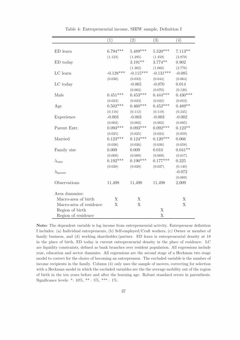
Table 4: Entrepreneurial income, SHIW sample, Definition I

(1) (2) (3) (4)

ED learn 6.794*** 5.489*** 5.520*** 7.113**(1.123) (1.295) (1.459) (2.879)

ED today 3.191** 3.774** 0.902(1.262) (1.660) (2.776)

LC learn -0.128*** -0.115*** -0.131*** -0.085(0.030) (0.033) (0.044) (0.064)

LC today -0.065 -0.070 0.014(0.062) (0.070) (0.120)

Male 0.451*** 0.453*** 0.444*** 0.430***(0.023) (0.023) (0.022) (0.053)

Age 0.502*** 0.460*** 0.452*** 0.489**(0.110) (0.112) (0.119) (0.245)

Experience -0.003 -0.003 -0.003 -0.002(0.002) (0.002) (0.002) (0.005)

Parent Entr. 0.093*** 0.093*** 0.092*** 0.123**(0.025) (0.025) (0.024) (0.059)

Married 0.123*** 0.124*** 0.120*** 0.066(0.026) (0.026) (0.026) (0.058)

Family size 0.009 0.009 0.010 0.041**(0.009) (0.009) (0.009) (0.017)

λentr 0.192*** 0.190*** 0.177*** 0.225(0.028) (0.028) (0.027) (0.140)

λmover -0.072(0.069)

Observations 11,498 11,498 11,498 2,009

Area dummies:Macro-area of birth X X XMacro-area of residence X X XRegion of birth XRegion of residence X

Note: The dependent variable is log income from entrepreneurial activity. Entrepreneur definition

I includes: (a) Individual entrepreneurs, (b) Self-employed/Craft workers, (c) Owner or member of

family business, and (d) working shareholder/partner. ED learn is entrepreneurial density at 18

in the place of birth, ED today is current entrepreneurial density in the place of residence. LC

are liquidity constraints, defined as bank branches over resident population. All regressions include

year, education and sector dummies. All regressions are the second stage of a Heckman two stage

model to correct for the choice of becoming an entrepreneur. The excluded variable is the number of

income recipients in the family. Column (4) only uses the sample of movers, correcting for selection

with a Heckman model in which the excluded variables are the the average mobility out of the region

of birth in the ten years before and after the learning age. Robust standard errors in parenthesis.

Significance levels: *: 10%, ** : 5%, *** : 1%.

37

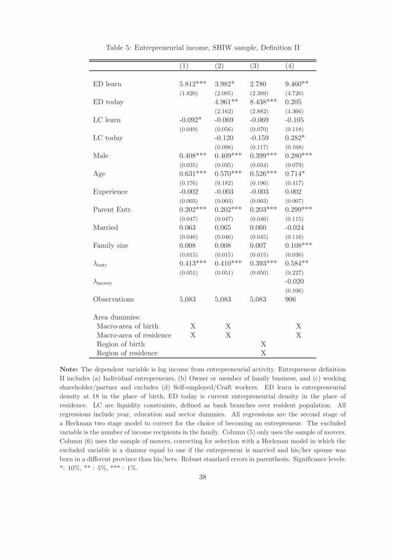
Table 5: Entrepreneurial income, SHIW sample, Definition II

(1) (2) (3) (4)

ED learn 5.812*** 3.982* 2.780 9.460**(1.820) (2.095) (2.389) (4.720)

ED today 4.961** 8.438*** 0.205(2.162) (2.882) (4.366)

LC learn -0.092* -0.069 -0.069 -0.105(0.049) (0.056) (0.070) (0.118)

LC today -0.120 -0.159 0.282*(0.098) (0.117) (0.168)

Male 0.408*** 0.409*** 0.399*** 0.280***(0.035) (0.035) (0.034) (0.079)

Age 0.631*** 0.570*** 0.526*** 0.714*(0.176) (0.182) (0.196) (0.417)

Experience -0.002 -0.003 -0.003 0.002(0.003) (0.003) (0.003) (0.007)

Parent Entr. 0.202*** 0.202*** 0.203*** 0.299***(0.047) (0.047) (0.046) (0.115)

Married 0.063 0.065 0.060 -0.024(0.046) (0.046) (0.045) (0.116)

Family size 0.008 0.008 0.007 0.108***(0.015) (0.015) (0.015) (0.030)

λentr 0.413*** 0.410*** 0.393*** 0.584**(0.051) (0.051) (0.050) (0.227)

λmover -0.020(0.106)

Observations 5,083 5,083 5,083 906

Area dummies:Macro-area of birth X X XMacro-area of residence X X XRegion of birth XRegion of residence X

Note: The dependent variable is log income from entrepreneurial activity. Entrepreneur definition

II includes (a) Individual entrepreneurs, (b) Owner or member of family business, and (c) working

shareholder/partner and excludes (d) Self-employed/Craft workers. ED learn is entrepreneurial

density at 18 in the place of birth, ED today is current entrepreneurial density in the place of

residence. LC are liquidity constraints, defined as bank branches over resident population. All

regressions include year, education and sector dummies. All regressions are the second stage of

a Heckman two stage model to correct for the choice of becoming an entrepreneur. The excluded

variable is the number of income recipients in the family. Column (5) only uses the sample of movers.

Column (6) uses the sample of movers, correcting for selection with a Heckman model in which the

excluded variable is a dummy equal to one if the entrepreneur is married and his/her spouse was

born in a different province than his/hers. Robust standard errors in parenthesis. Significance levels:

*: 10%, ** : 5%, *** : 1%.

38

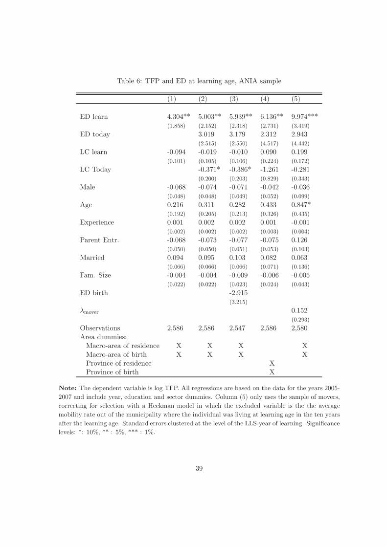
Table 6: TFP and ED at learning age, ANIA sample

(1) (2) (3) (4) (5)

ED learn 4.304** 5.003** 5.939** 6.136** 9.974***(1.858) (2.152) (2.318) (2.731) (3.419)

ED today 3.019 3.179 2.312 2.943(2.515) (2.550) (4.517) (4.442)

LC learn -0.094 -0.019 -0.010 0.090 0.199(0.101) (0.105) (0.106) (0.224) (0.172)

LC Today -0.371* -0.386* -1.261 -0.281(0.200) (0.203) (0.829) (0.343)

Male -0.068 -0.074 -0.071 -0.042 -0.036(0.048) (0.048) (0.049) (0.052) (0.099)

Age 0.216 0.311 0.282 0.433 0.847*(0.192) (0.205) (0.213) (0.326) (0.435)

Experience 0.001 0.002 0.002 0.001 -0.001(0.002) (0.002) (0.002) (0.003) (0.004)

Parent Entr. -0.068 -0.073 -0.077 -0.075 0.126(0.050) (0.050) (0.051) (0.053) (0.103)

Married 0.094 0.095 0.103 0.082 0.063(0.066) (0.066) (0.066) (0.071) (0.136)

Fam. Size -0.004 -0.004 -0.009 -0.006 -0.005(0.022) (0.022) (0.023) (0.024) (0.043)

ED birth -2.915(3.215)

λmover 0.152(0.293)

Observations 2,586 2,586 2,547 2,586 2,580Area dummies:Macro-area of residence X X X XMacro-area of birth X X X XProvince of residence XProvince of birth X

Note: The dependent variable is log TFP. All regressions are based on the data for the years 2005-

2007 and include year, education and sector dummies. Column (5) only uses the sample of movers,

correcting for selection with a Heckman model in which the excluded variable is the the average

mobility rate out of the municipality where the individual was living at learning age in the ten years

after the learning age. Standard errors clustered at the level of the LLS-year of learning. Significance

levels: *: 10%, ** : 5%, *** : 1%.

39

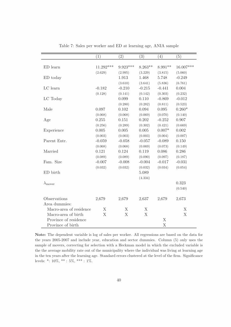
Table 7: Sales per worker and ED at learning age, ANIA sample

(1) (2) (3) (4) (5)

ED learn 11.292*** 9.923*** 8.263** 8.991** 16.007***(2.629) (2.995) (3.229) (3.815) (5.060)

ED today 1.913 1.468 5.748 -0.249(3.610) (3.641) (5.836) (6.761)

LC learn -0.182 -0.210 -0.215 -0.441 0.004(0.128) (0.141) (0.142) (0.303) (0.232)

LC Today 0.099 0.110 -0.869 -0.012(0.280) (0.282) (0.811) (0.523)

Male 0.097 0.102 0.094 0.095 0.260*(0.068) (0.068) (0.069) (0.070) (0.140)

Age 0.255 0.151 0.202 -0.252 0.907(0.256) (0.289) (0.302) (0.421) (0.669)

Experience 0.005 0.005 0.005 0.007* 0.002(0.003) (0.003) (0.003) (0.004) (0.007)

Parent Entr. -0.059 -0.058 -0.057 -0.089 0.150(0.068) (0.068) (0.069) (0.073) (0.149)

Married 0.121 0.124 0.119 0.086 0.286(0.089) (0.089) (0.090) (0.097) (0.187)

Fam. Size -0.007 -0.008 -0.004 -0.017 -0.031(0.032) (0.032) (0.032) (0.034) (0.054)

ED birth 5.089(4.334)

λmover 0.323(0.540)

Observations 2,679 2,679 2,637 2,679 2,673Area dummies:Macro-area of residence X X X XMacro-area of birth X X X XProvince of residence XProvince of birth X

Note: The dependent variable is log of sales per worker. All regressions are based on the data for

the years 2005-2007 and include year, education and sector dummies. Column (5) only uses the

sample of movers, correcting for selection with a Heckman model in which the excluded variable is

the the average mobility rate out of the municipality where the individual was living at learning age

in the ten years after the learning age. Standard errors clustered at the level of the firm. Significance

levels: *: 10%, ** : 5%, *** : 1%.

40

Table 8: Descriptive statistics, traits, managerial practices and innovation

Variable Obs Mean Std. Dev. Min MaxPanel A: Traits

Risk aversion 966 2.70 .67 1 4Ambiguity aversion 954 3.40 1.44 1 5Confidence 944 2.18 .40 1 3Optimism 946 7.33 1.76 0 10Satisfaction 935 7.47 1.67 0 10

Panel B: Innovation

Share innov. 736 17.43 24.46 0 100Innov. practices 388 2.09 1.2 1 5

Panel C: Managerial practices

Management 388 2.41 .66 1 4.41Monitoring 388 2.67 .82 1 5Targets 388 2.41 .90 1 5People 388 2.33 .64 1 5

Note: See appendix A.3 for the definition of the variables.

41

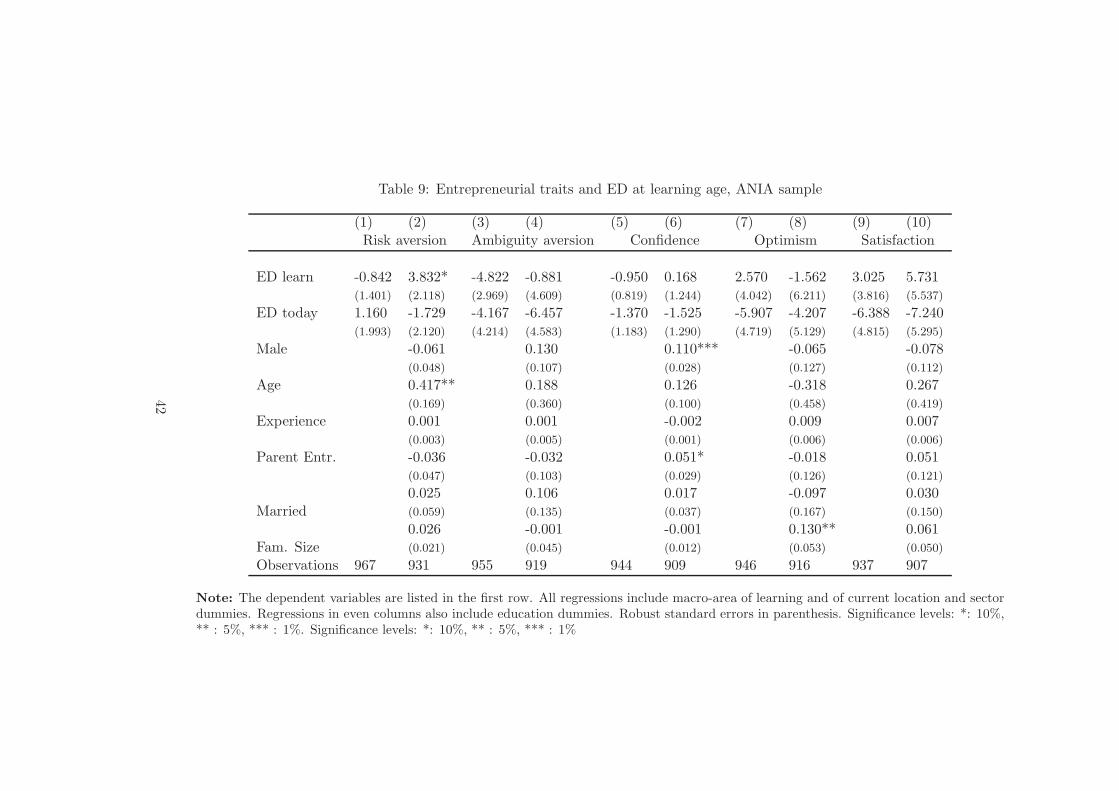
Table 9: Entrepreneurial traits and ED at learning age, ANIA sample

(1) (2) (3) (4) (5) (6) (7) (8) (9) (10)Risk aversion Ambiguity aversion Confidence Optimism Satisfaction

ED learn -0.842 3.832* -4.822 -0.881 -0.950 0.168 2.570 -1.562 3.025 5.731(1.401) (2.118) (2.969) (4.609) (0.819) (1.244) (4.042) (6.211) (3.816) (5.537)

ED today 1.160 -1.729 -4.167 -6.457 -1.370 -1.525 -5.907 -4.207 -6.388 -7.240(1.993) (2.120) (4.214) (4.583) (1.183) (1.290) (4.719) (5.129) (4.815) (5.295)

Male -0.061 0.130 0.110*** -0.065 -0.078(0.048) (0.107) (0.028) (0.127) (0.112)

Age 0.417** 0.188 0.126 -0.318 0.267(0.169) (0.360) (0.100) (0.458) (0.419)

Experience 0.001 0.001 -0.002 0.009 0.007(0.003) (0.005) (0.001) (0.006) (0.006)

Parent Entr. -0.036 -0.032 0.051* -0.018 0.051(0.047) (0.103) (0.029) (0.126) (0.121)

0.025 0.106 0.017 -0.097 0.030Married (0.059) (0.135) (0.037) (0.167) (0.150)

0.026 -0.001 -0.001 0.130** 0.061Fam. Size (0.021) (0.045) (0.012) (0.053) (0.050)

Observations 967 931 955 919 944 909 946 916 937 907

Note: The dependent variables are listed in the first row. All regressions include macro-area of learning and of current location and sectordummies. Regressions in even columns also include education dummies. Robust standard errors in parenthesis. Significance levels: *: 10%,** : 5%, *** : 1%. Significance levels: *: 10%, ** : 5%, *** : 1%

42

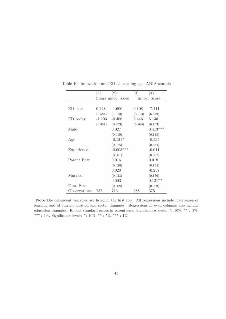
Table 10: Innovation and ED at learning age, ANIA sample

(1) (2) (3) (4)Share innov. sales Innov. Score

ED learn 0.248 -1.600 0.108 -7.111(0.584) (1.010) (3.913) (6.379)

ED today -1.103 -0.466 2.446 6.130(0.851) (0.973) (5.768) (6.153)

Male 0.027 0.413***(0.019) (0.148)

Age -0.131* -0.535(0.075) (0.484)

Experience -0.003*** -0.011(0.001) (0.007)

Parent Entr. 0.016 0.018(0.020) (0.134)

0.020 -0.257Married (0.023) (0.176)

0.003 0.121**Fam. Size (0.008) (0.059)

Observations 737 713 388 375

Note:The dependent variables are listed in the first row. All regressions include macro-area of

learning and of current location and sector dummies. Regressions in even columns also include

education dummies. Robust standard errors in parenthesis. Significance levels: *: 10%, ** : 5%,

*** : 1%. Significance levels: *: 10%, ** : 5%, *** : 1%

43

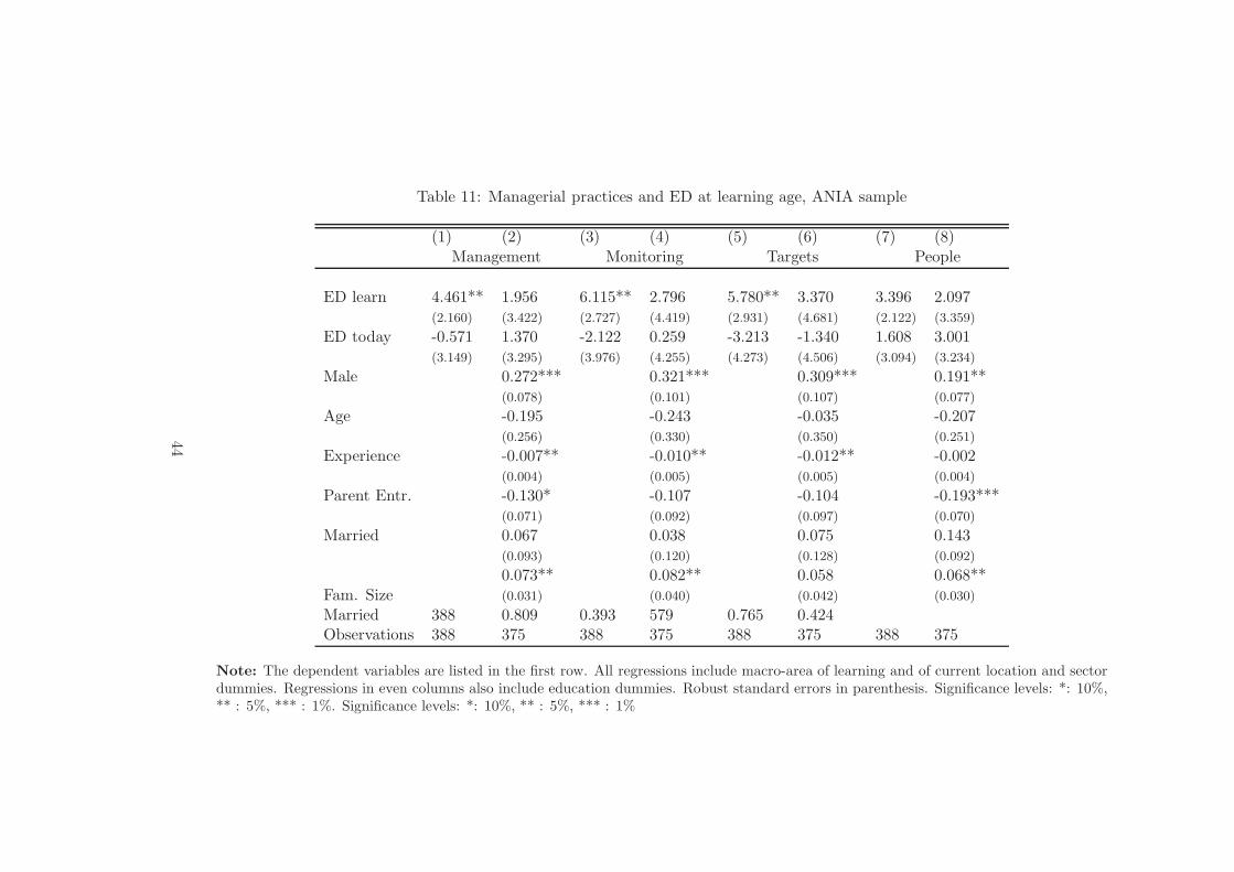
Table 11: Managerial practices and ED at learning age, ANIA sample

(1) (2) (3) (4) (5) (6) (7) (8)Management Monitoring Targets People

ED learn 4.461** 1.956 6.115** 2.796 5.780** 3.370 3.396 2.097(2.160) (3.422) (2.727) (4.419) (2.931) (4.681) (2.122) (3.359)

ED today -0.571 1.370 -2.122 0.259 -3.213 -1.340 1.608 3.001(3.149) (3.295) (3.976) (4.255) (4.273) (4.506) (3.094) (3.234)

Male 0.272*** 0.321*** 0.309*** 0.191**(0.078) (0.101) (0.107) (0.077)

Age -0.195 -0.243 -0.035 -0.207(0.256) (0.330) (0.350) (0.251)

Experience -0.007** -0.010** -0.012** -0.002(0.004) (0.005) (0.005) (0.004)

Parent Entr. -0.130* -0.107 -0.104 -0.193***(0.071) (0.092) (0.097) (0.070)

Married 0.067 0.038 0.075 0.143(0.093) (0.120) (0.128) (0.092)

0.073** 0.082** 0.058 0.068**Fam. Size (0.031) (0.040) (0.042) (0.030)

Married 388 0.809 0.393 579 0.765 0.424Observations 388 375 388 375 388 375 388 375

Note: The dependent variables are listed in the first row. All regressions include macro-area of learning and of current location and sectordummies. Regressions in even columns also include education dummies. Robust standard errors in parenthesis. Significance levels: *: 10%,** : 5%, *** : 1%. Significance levels: *: 10%, ** : 5%, *** : 1%

44

A Appendix: Data details

A.1 The ANIA survey

The ANIA Survey for Small Business Companies collects data on a sample of 2,295 Italian

firms and their top manager. The survey was conducted on a sample of small Italian firms,

having up to a maximum of 250 employees, extracted from the total number of companies

registered with CERVED - a business information agency operating in Italy which collects

companies balance sheet data. The survey was conducted between October 2008 and July

2009.

Compared to the initial target set at the completion of 2,300 interviews, the investigation

closed with 2,295 completed interviews. Participation in the survey entails the willingness

to provide detailed information regarding many aspects of the firm’s operations and char-

acteristics as well as the willingness of the CEO/owner of the company to take part in a

face-to-face interview with a professional interviewer. The first type of data was collected

through a questionnaire filled out by each company, while the second type was obtained

through an interview using the Computer Assisted Personal Interviewing method. Partly

because the survey took place during the financial crisis and partly because interviews tar-

geted the CEO of the firm, the drop out rate was relatively high particularly among firms

in the larger size categories. To account for this the survey design was slightly reviewed to

include a larger number of smaller firms (with less than 20 employees) which were easier

targets. This has caused the sample to be somewhat biased towards smaller firms than the

population of businesses with up to 250 employees.

A.2 The managerial practices survey

The data collection is based on a telephone double-blind survey technique and comprises

a set of open-ended questions that are subsequently evaluated using a scoring grid. Qual-

itative answers are then recoded into quantitative measures with a score ranging between

1 (worst) to 5 (best managerial practices). We first set up a group of interviewers, trained

them with a specific program and then had them run the survey. The data collection pro-

cess was carried out using the methodology of the World Management Survey,

http://www.worldmanagementsurvey.com/See Bloom and Van Reenen (2010a) and Bloom

et al. (2012) for a full exposition of the survey characteristics and the data collection method.

Not all firms that were re-contacted participated to the management survey. A com-

parison of the observable characteristics of those who refused to participate and those who

participated shows no systematic differences in terms of firm characteristics, sector, area of

location and of learning. Some small but statistically significant differences emerge in terms

of entrepreneurs’ characteristics, such as education and having at least one parent that was

an entrepreneur (see Table A.2.

45

A.3 Variables definition

Here we provide a detailed description of the variables used in the paper whose definitions

are not obvious.

• Entrepreneur, Def. I This is a broaded definition which includes: self employed,

partners of a company and owners that run an incorporated business.

• Entrepreneur, Def. II This is a narrowed definition that only include partners of a

company and owners that run an incorporated business.

• ED learn Entrepreneurial density (number of firms per capita) in the location where

the entrepreneur was living at age 18.

• ED today Current entrepreneurial density (number of firms per capita) in the location

where the entrepreneur (or the firm in the case of the ANIA sample) is located.

• LC learn Log of bank branches per capita in the location where the entrepreneur was

living at age 18. In Table 1 we report the mean and standard deviation of the level

(rather than the log) of branches per 1000 inhabitants.

• LC today Log of current bank branches per capita in the location where the en-

trepreneur (or the firm in the case of the ANIA sample) is located. In Table 1 we

report the mean and standard deviation of the level (rather than the log) of branches

per 1000 inhabitants.

• Number of income recipients Members of the household who receive some income.

• Mover A dummy equal to 1 if current location of the individual is different from

that in which she was born (SHIW sample) or was living at 18 (ANIA sample). In

the SHIW sample, we distinguish between all individuals (Mover) and Entrepreneurs

(Mover-Entrepreneur).

• Years in control : Number of years since the entrepreneur has acquired the responsi-

bility of the management of the firm.

• Risk aversion: Indicator obtained using the answers to the question: “If the in-

vestment strategy of the firm depends only on you, among the following alternative

strategies which one would you pick up? One that yields a) Low profits but no risk of

losses; b) Decent profits and rare losses; c) Good profits with some chances of incur-

ring losses; d) Very high profits with a high risk of significant losses.” The indicator

is coded between 1 and 4, increasing in risk aversion.

• Ambiguity aversion Indicator obtained using the answers to the question: “Think

about two urns, each containing 100 balls, either green or yellow. You win 1,000 euros

if you draw an urn of the color of your choice. Choose the color. Urn 1 contains both

46

green and yellow balls, in unknown proportion. Urn 2 contains 50 green and 50 yellow

balls. From which urn would you rather draw the ball? a) Strong preference for urn

1; b) slight preference for urn 1; c) indifferent; d) slight preference for urn 2; e) strong

preference for urn 2.” The indicator is coded between 1 and 5, increasing in ambiguity

aversion.

• Confidence Indicator obtained using the answers to the question: “With respect to

the average ability of other entrepreneurs, in your job, do you believe to be: a) below

average; b) average; c) above average.” The indicator is coded between 1 and 3,

increasing in self confidence.

• Optimism: answers to the question borrowed from a standard Life Orientation Test

(Scheier et al., 1994): “How much do you agree with the statement: Overall I expect

more good things than bad things to happen to me”. Coded between 0 and 10, with

a higher number indicating more optimism.

• Satisfaction: Indicator obtained from the following question: “Notwithstanding the

profits motive and only considering the other characteristics of your job, can you tell

me if they give you more satisfaction or dissatisfaction?” Coded between 0 and 10,

with a higher number indicating more satisfaction.

• Share of innov.: Log of 1+ the share of sales in 2007 due to products or services either

new or substantially improved, introduced to the market between 2005 and 2007.

47

Table A.1: First stage regressions for movers

SHIW ANIA

ED learn -4.743*** 6.484(0.546) (5.121)

ED today 3.022*** -0.732(0.661) (5.563)

LC learn -0.020 0.101(0.014) (0.221)

LC today 0.063* 0.527(0.036) (0.0411)

Male -0.015** 0.010(0.007) (0.103)

Age -0.137*** 0.864**(0.041) (0.440)

Experience 0.001 -0.004(0.001) (0.005)

Parent Entr. -0.019** -0.129(0.008) (0.100)

Married 0.036*** -0.286**(0.007) (0.124)

Family size -0.007** 0.023(0.003) (0.044)

N. income -0.010***recepients (0.004)

Local mobility 8.324*** 29.607**next 10 years (2.597) (14.594)

Local mobility -6.336***past 10 years (2.365)

Observations 60,318 2,580

Note: the table reports the first stage probit regression in the Heckman selection model forthe SHIW and ANIA sample. The dependent variable is a dummy equal to 1 for individualsthat are currently resident in a province different form that of birth (SHIW) or in a LLSdifferent from that in which the individual was living at 18 (ANIA). Local Mobility is themobility rate out of the region (SHIW) or out of the municipality (ANIA). Next ten or pastten years refer to the average mobility at the local level in the ten years before or after theyear in which the individual was 18. Both regressions include dummies for year, education,sector, macro area of birth (SHIW)/of learning (ANIA) and of current residence.

48

Table A.2: Comparison between re-interviewed and non re-interviewed entrepreneurs

Re-interviewed Non re-interviewed

N. Obs. Mean Std. Dev. N. Obs. Mean Std. Dev. Difference

TFP 388 2.511 0.836 579 2.416 0.948 0.096Sales per worker 388 4.941 1.069 575 4.867 1.245 0.074Employees 388 36.503 40.175 579 32.824 40.477 3.679Dumsect1 388 0.036 0.187 579 0.024 0.154 0.012Dumsect2 388 0.381 0.486 579 0.337 0.473 0.045Dumsect3 388 0.010 0.101 579 0.009 0.093 0.002Dumsect4 388 0.046 0.211 579 0.098 0.298 -0.052***Dumsect5 388 0.240 0.427 579 0.247 0.432 0.007Dumsect6 388 0.034 0.180 579 0.048 0.215 -0.015Dumsect7 388 0.253 0.435 579 0.237 0.425 0.016Dumarea1 388 0.307 0.462 579 0.316 0.465 -0.009Dumarea2 388 0.302 0.460 579 0.297 0.457 0.004Dumarea3 388 0.209 0.407 579 0.192 0.394 0.017Dumarea4 388 0.183 0.387 579 0.195 0.397 -0.012Dumarealearn1 388 0.291 0.455 579 0.314 0.465 -0.023Dumarealearn2 388 0.291 0.455 579 0.287 0.453 0.005Dumarealearn3 388 0.216 0.412 579 0.174 0.380 0.042Dumarealearn4 388 0.201 0.401 579 0.225 0.418 -0.023Education 388 14.031 2.570 579 13.377 2.547 0.654***Age 388 51.716 11.107 579 50.421 10.119 1.295*Male 388 0.722 0.449 579 0.663 0.473 0.058*Parent Entr. 388 0.451 0.498 579 0.359 0.480 0.092***Experience 388 20.649 11.301 579 19.036 10.868 1.613**Married 388 0.809 0.393 579 0.765 0.424 0.044Family size 375 3.093 1.197 556 3.043 1.159 0.050

Note: the table reports means and standard deviations of key variables for the sample of en-

trepreneurs that were re-interviewed and that were not. The last column report differences in mean.∗∗∗ indicates significantly different at 1%, ∗∗ at 5%, ∗ at 10%.

49

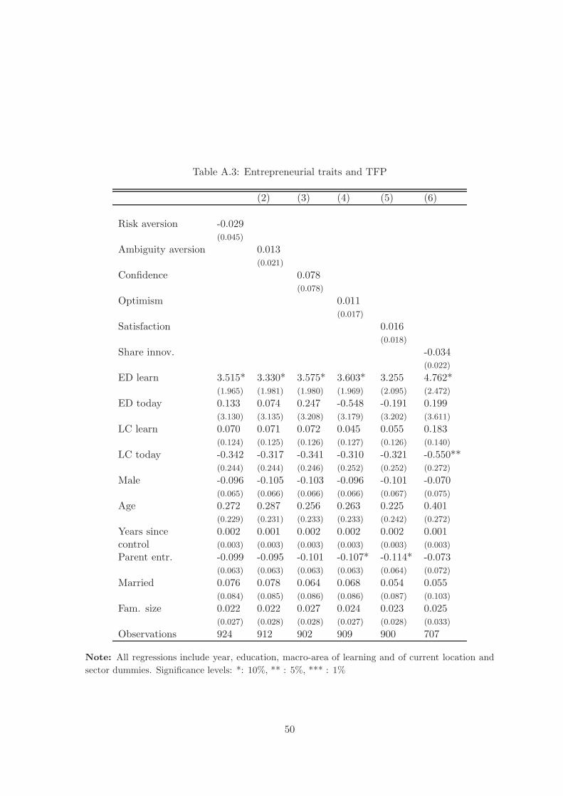
Table A.3: Entrepreneurial traits and TFP

(2) (3) (4) (5) (6)

Risk aversion -0.029(0.045)

Ambiguity aversion 0.013(0.021)

Confidence 0.078(0.078)

Optimism 0.011(0.017)

Satisfaction 0.016(0.018)

Share innov. -0.034(0.022)

ED learn 3.515* 3.330* 3.575* 3.603* 3.255 4.762*(1.965) (1.981) (1.980) (1.969) (2.095) (2.472)

ED today 0.133 0.074 0.247 -0.548 -0.191 0.199(3.130) (3.135) (3.208) (3.179) (3.202) (3.611)

LC learn 0.070 0.071 0.072 0.045 0.055 0.183(0.124) (0.125) (0.126) (0.127) (0.126) (0.140)

LC today -0.342 -0.317 -0.341 -0.310 -0.321 -0.550**(0.244) (0.244) (0.246) (0.252) (0.252) (0.272)

Male -0.096 -0.105 -0.103 -0.096 -0.101 -0.070(0.065) (0.066) (0.066) (0.066) (0.067) (0.075)

Age 0.272 0.287 0.256 0.263 0.225 0.401(0.229) (0.231) (0.233) (0.233) (0.242) (0.272)

Years since 0.002 0.001 0.002 0.002 0.002 0.001control (0.003) (0.003) (0.003) (0.003) (0.003) (0.003)

Parent entr. -0.099 -0.095 -0.101 -0.107* -0.114* -0.073(0.063) (0.063) (0.063) (0.063) (0.064) (0.072)

Married 0.076 0.078 0.064 0.068 0.054 0.055(0.084) (0.085) (0.086) (0.086) (0.087) (0.103)

Fam. size 0.022 0.022 0.027 0.024 0.023 0.025(0.027) (0.028) (0.028) (0.027) (0.028) (0.033)

Observations 924 912 902 909 900 707

Note: All regressions include year, education, macro-area of learning and of current location and

sector dummies. Significance levels: *: 10%, ** : 5%, *** : 1%

50

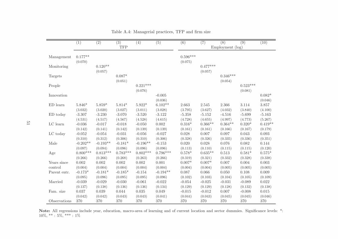
Table A.4: Managerial practices, TFP and firm size

(1) (2) (3) (4) (5) (6) (7) (8) (9) (10)TFP Employment (log)

Management 0.177** 0.596***(0.070) (0.075)

Monitoring 0.120** 0.477***(0.057) (0.057)

Targets 0.087* 0.346***(0.051) (0.054)

People 0.221*** 0.523***(0.076) (0.081)

Innovation -0.005 0.082*(0.036) (0.046)

ED learn 5.846* 5.859* 5.814* 5.922* 6.102** 2.663 2.545 2.366 3.114 3.857(3.032) (3.020) (3.027) (3.011) (3.028) (3.795) (3.627) (4.032) (3.840) (4.100)

ED today -3.307 -3.230 -3.070 -3.520 -3.122 -5.358 -5.152 -4.516 -5.699 -5.163(4.531) (4.517) (4.567) (4.528) (4.615) (4.728) (4.655) (4.997) (4.773) (5.267)

LC learn -0.036 -0.017 -0.018 -0.050 0.002 0.316* 0.366** 0.364** 0.320* 0.419**(0.142) (0.141) (0.142) (0.139) (0.139) (0.161) (0.161) (0.166) (0.167) (0.179)

LC today -0.052 -0.054 -0.031 -0.056 -0.027 0.028 0.007 0.097 0.043 0.093(0.310) (0.312) (0.306) (0.310) (0.306) (0.328) (0.326) (0.335) (0.336) (0.351)

Male -0.202** -0.193** -0.181* -0.196** -0.153 0.020 0.028 0.076 0.082 0.144(0.097) (0.094) (0.096) (0.096) (0.096) (0.113) (0.110) (0.115) (0.115) (0.120)

Age 0.800*** 0.813*** 0.783*** 0.802*** 0.796*** 0.578* 0.635** 0.513 0.581* 0.575*(0.266) (0.266) (0.268) (0.263) (0.266) (0.319) (0.321) (0.332) (0.328) (0.338)

Years since 0.002 0.002 0.002 0.002 0.001 0.007* 0.007* 0.007 0.004 0.003control (0.004) (0.004) (0.004) (0.004) (0.004) (0.004) (0.004) (0.005) (0.005) (0.005)

Parent entr. -0.173* -0.181* -0.185* -0.154 -0.194** 0.087 0.066 0.050 0.108 0.009(0.095) (0.096) (0.095) (0.095) (0.096) (0.102) (0.103) (0.104) (0.105) (0.109)

Married -0.039 -0.029 -0.030 -0.061 -0.022 -0.054 -0.025 -0.031 -0.089 0.022(0.137) (0.138) (0.136) (0.136) (0.134) (0.129) (0.129) (0.128) (0.132) (0.138)

Fam. size 0.037 0.039 0.044 0.035 0.049 -0.015 -0.012 0.007 -0.008 0.015(0.042) (0.042) (0.043) (0.043) (0.041) (0.044) (0.043) (0.045) (0.045) (0.046)

Observations 370 370 370 370 370 370 370 370 370 370

Note: All regressions include year, education, macro-area of learning and of current location and sector dummies. Significance levels: *:10%, ** : 5%, *** : 1%

51