Learning Discriminative Models with Incomplete

Data

by

Ashish Kapoor

B. Tech., Indian Institute of Technology, Delhi (2000)S. M., Massachusetts Institute of Technology (2002)

Submitted to the Program in Media Arts and Sciences,School of Architecture and Planning

in partial fulfillment of the requirements for the degree of

Doctor of Philosophy in Media Arts and Sciences

at the

MASSACHUSETTS INSTITUTE OF TECHNOLOGY

February 2006

c© Massachusetts Institute of Technology 2006. All rights reserved.

Author . . . . . . . . . . . . . . . . . . . . . . . . . . . . . . . . . . . . . . . . . . . . . . . . . . . . . . . . . . . . . .Program in Media Arts and Sciences,School of Architecture and Planning

January 13, 2006

Certified by. . . . . . . . . . . . . . . . . . . . . . . . . . . . . . . . . . . . . . . . . . . . . . . . . . . . . . . . . .Rosalind W. Picard

Professor of Media Arts and SciencesThesis Supervisor

Accepted by . . . . . . . . . . . . . . . . . . . . . . . . . . . . . . . . . . . . . . . . . . . . . . . . . . . . . . . . .Andrew B. Lippman

ChairmanDepartment Committee on Graduate Students

2

Learning Discriminative Models with Incomplete Databy

Ashish Kapoor

Submitted to the Program in Media Arts and Sciences,School of Architecture and Planning

on January 13, 2006, in partial fulfillment of therequirements for the degree of

Doctor of Philosophy in Media Arts and Sciences

Abstract

Many practical problems in pattern recognition require making inferences using mul-tiple modalities, e.g. sensor data from video, audio, physiological changes etc. Oftenin real-world scenarios there can be incompleteness in the training data. There canbe missing channels due to sensor failures in multi-sensory data and many data pointsin the training set might be unlabeled. Further, instead of having exact labels wemight have easy to obtain coarse labels that correlate with the task. Also, there canbe labeling errors, for example human annotation can lead to incorrect labels in thetraining data.

The discriminative paradigm of classification aims to model the classificationboundary directly by conditioning on the data points; however, discriminative mod-els cannot easily handle incompleteness since the distribution of the observations isnever explicitly modeled. We present a unified Bayesian framework that extends thediscriminative paradigm to handle four different kinds of incompleteness. First, asolution based on a mixture of Gaussian processes is proposed for achieving sensorfusion under the problematic conditions of missing channels. Second, the frameworkaddresses incompleteness resulting from partially labeled data using input dependentregularization. Third, we introduce the located hidden random field (LHRF) thatlearns finer level labels when only some easy to obtain coarse information is avail-able. Finally the proposed framework can handle incorrect labels, the fourth case ofincompleteness. One of the advantages of the framework is that we can use differentmodels for different kinds of label errors, providing a way to encode prior knowledgeabout the process.

The proposed extensions are built on top of Gaussian process classification andresult in a modular framework where each component is capable of handling differentkinds of incompleteness. These modules can be combined in many different ways,resulting in many different algorithms within one unified framework. We demonstratethe effectiveness of the framework on a variety of problems such as multi-sensor affectrecognition, image classification and object detection and segmentation.

Thesis Supervisor: Rosalind W. PicardTitle: Professor of Media Arts and Sciences

3

4

Learning Discriminative Models with Incomplete Databy

Ashish Kapoor

Thesis Committee:

Advisor . . . . . . . . . . . . . . . . . . . . . . . . . . . . . . . . . . . . . . . . . . . . . . . . . . . . . . . . . . . . . . . . . . . . . . . . . . . .Rosalind W. Picard

Professor of Media Arts and SciencesMassachusetts Institute of Technology

Thesis Reader . . . . . . . . . . . . . . . . . . . . . . . . . . . . . . . . . . . . . . . . . . . . . . . . . . . . . . . . . . . . . . . . . . . . .Eric Horvitz

Senior ResearcherMicrosoft Research

Thesis Reader . . . . . . . . . . . . . . . . . . . . . . . . . . . . . . . . . . . . . . . . . . . . . . . . . . . . . . . . . . . . . . . . . . . . .Joshua Tenenbaum

Paul E. Newton Assistant Professor of Computational Cognitive ScienceMassachusetts Institute of Technology

5

6

Acknowledgments

I would like to thank Rosalind W. Picard, my wonderful advisor and a great sourceof inspiration. Thank you Roz for bringing me to MIT in the first place and for beingso patient and supportive all these years. I thank Eric Horvitz and Josh Tenenbaumfor being readers for this thesis. Thanks to Eric for his inspiring ideas, enthusiasmand critique about the work. Thanks to Josh for his insight, motivation and support.

I wish to thank all the folks who helped with this thesis. Special thanks to JohnWinn, my mentor and collaborator at Microsoft Research, Cambridge. It was John’sinsight and guidance that led to the work on Located Hidden Random Fields forobject detection and segmentation. Thanks to Yuan (Alan) Qi for his guidance andinsight with much of the work on semi-supervised learning mentioned in this thesis.Thanks to Yuri Ivanov, whose work on classifier combination inspired the work onmultimodal affect recognition. Also, many thanks to Tom Minka who has tirelesslyanswered all my stupid and not so stupid questions on machine learning. I especiallywish to thank Sumit Basu and Tanzeem Choudhury, my mentors, collaborators andfriends. Thank you Sumit for the best summer internship I ever had. Thank youTanzeem for being such a great friend and a mentor. There have been many othercollaborators including Hyungil Ahn and Rana El Kaliouby whom I’d like to thank.There have been many UROPs who have burnt their midnight oil: Yue-Hann Chin,Timothy Heidel, Heather Knight, David Lafferty, Christine Lin, Louis Lopez andDavid Lopez Mateos. I’d also like to thank Sandy Pentland and Trevor Darrell whohave inspired and motivated me with their advice, guidance and council.

Thanks to Rgrads past and present: Tim Bickmore, Win Burleson, Shani Daily,Raul Fernandez, Karen Liu, Akshay Mohan, Selene Mota, Yuan Qi, Seth Raphael,Carson Reynolds, Jay Silver and Alea Teeters. It was a great group to work with.Thanks to the friends at the Media Lab and CSAIL who have enriched my graduatestudent life with their insight and invaluable council. I mention a few of them here:Juan Carlos Barahona, Neal Checka, Brian Clarkson, Nathan Eagle, Mary Farbood,Tony Jebara, Aisling Kelliher, Vikram Sheel Kumar, Hyun-Yeul Lee, Andrea LockerdThomaz, Louis-Philippe Morency, Paul Nemirovsky, Ali Rahimi, Ben Recht, GregoryShakhnarovich and Kevin Wilson.

Thanks to all my friends who stood by me all the time. Special thanks to theBoston mafia: Vishwanath Anantraman, Aarthi Chandrasekaran, Rupa Das, ManishDeopura, Joyce George, Vipin Gupta, Mahesh Kumar, Ashish Nimgaonkar, AnandRajgopal, Anoop Rao, Neha Soni, Kunal Surana, Kushan Surana, Sapna Tyagi, Chin-tan Vaishnav, Hetal Vaishnav and Charuleka Varadharajan. I cant imagine how mylife for the past six years would have been without them. Also, I was lucky to meetJulian Lange, Anurag Chandra, Ayla Ergun, Kate Lesnaia, Erin Maneri and AnshulSood, my first friends in Boston. It was they who help me adjust to the Americanlifestyle when I first moved and have influenced my life in many great ways. Spe-cial thanks to Lucy Wong for being a constant source of enthusiasm and inspiration(and also for letting me take 402B). Also, special thanks to Jon Kennell, my apart-ment mate for two years. The days with Mango Lazy were the best. Thanks toMatt Lehman and Helana, our Gwen Stefani during Mango Lazy’s early days. I also

7

wish to thank my close friends from IIT Delhi: Ankit Bal, Rohit Dube, Nikhil Garg,Dhaval Gothi, Sachin Jain, Hatinder Madan, Saurabh Mahajan, Dheeraj Malhotra,Ankur Mani and Alok Ranjan. Thank you guys for being with me always. Its theywho made a punster out of me so that I could see the funnier side of life.

A very special thanks to my aunt Maya Das and my uncle Dilip Das. They weremy family and took care of my well being all these years. A visit to Bedford was likea visit to home. Thanks to Geeta jaithai, Mukut jetpeha and Bipu dada, my earliestinspirations. Thanks to my family and friends back from home in India and thereare so many others I wish to thank. Finally, thanks to Ma, Baba and my little sisterAakashi for their unconditional love and support. It was their strength and prayersthat always carried me through the toughest times.

8

Contents

1 Introduction 191.1 Types of Incompleteness . . . . . . . . . . . . . . . . . . . . . . . . . 20

1.1.1 Other Types of Incompleteness . . . . . . . . . . . . . . . . . 211.2 Contributions of the Thesis . . . . . . . . . . . . . . . . . . . . . . . 221.3 Thesis Outline . . . . . . . . . . . . . . . . . . . . . . . . . . . . . . . 25

2 Gaussian Process Classification with Noisy Labels 292.1 Gaussian Process Classification . . . . . . . . . . . . . . . . . . . . . 29

2.1.1 Gaussian Process Priors . . . . . . . . . . . . . . . . . . . . . 312.1.2 Classification Likelihoods to Handle Noisy Labels . . . . . . . 31

2.2 Approximate Bayesian Inference . . . . . . . . . . . . . . . . . . . . . 352.2.1 Expectation Propagation for Gaussian Process Classification . 362.2.2 Representing the Posterior Mean and the Covariance . . . . . 38

2.3 Hyperparameter Learning . . . . . . . . . . . . . . . . . . . . . . . . 382.4 Experiments . . . . . . . . . . . . . . . . . . . . . . . . . . . . . . . . 402.5 Conclusions and Extensions . . . . . . . . . . . . . . . . . . . . . . . 46

3 Mixture of Gaussian Processes for Combining Multiple Modalities 493.1 Previous Work . . . . . . . . . . . . . . . . . . . . . . . . . . . . . . 503.2 Our Approach . . . . . . . . . . . . . . . . . . . . . . . . . . . . . . . 52

3.2.1 Gaussian Process Classification . . . . . . . . . . . . . . . . . 533.2.2 Mixture of Gaussian Processes for Sensor Fusion . . . . . . . . 553.2.3 A Toy Example . . . . . . . . . . . . . . . . . . . . . . . . . . 58

3.3 Multimodal Affect Recognition in Learning Environments . . . . . . . 593.3.1 System Overview . . . . . . . . . . . . . . . . . . . . . . . . . 603.3.2 Empirical Evaluation . . . . . . . . . . . . . . . . . . . . . . . 62

3.4 Conclusions and Future Work . . . . . . . . . . . . . . . . . . . . . . 66

4 Gaussian Process Classification with Partially Labeled Data 694.1 Previous Work . . . . . . . . . . . . . . . . . . . . . . . . . . . . . . 72

4.1.1 Semi-supervised Classification . . . . . . . . . . . . . . . . . . 724.1.2 Hyperparameter and Kernel Learning . . . . . . . . . . . . . . 73

4.2 Bayesian Semi-Supervised Learning . . . . . . . . . . . . . . . . . . . 744.2.1 Priors and Regularization on Graphs . . . . . . . . . . . . . . 744.2.2 The Likelihood . . . . . . . . . . . . . . . . . . . . . . . . . . 75

9

4.2.3 Approximate Inference . . . . . . . . . . . . . . . . . . . . . . 764.3 Hyperparameter Learning . . . . . . . . . . . . . . . . . . . . . . . . 76

4.3.1 Classifying New Points . . . . . . . . . . . . . . . . . . . . . . 774.4 Experiments . . . . . . . . . . . . . . . . . . . . . . . . . . . . . . . . 784.5 Connections to Gaussian Processes . . . . . . . . . . . . . . . . . . . 844.6 Connections to Other Approaches . . . . . . . . . . . . . . . . . . . . 864.7 Conclusion and Future Work . . . . . . . . . . . . . . . . . . . . . . . 88

5 Located Hidden Random Fields to Learn Discriminative Parts 895.1 Relation to Gaussian Process Classification . . . . . . . . . . . . . . . 905.2 Learning Discriminative Parts for Object Detection and Segmentation 905.3 Related Work . . . . . . . . . . . . . . . . . . . . . . . . . . . . . . . 915.4 Discriminative Models for Object Detection . . . . . . . . . . . . . . 92

5.4.1 Located Hidden Random Field . . . . . . . . . . . . . . . . . 945.5 Inference and Learning . . . . . . . . . . . . . . . . . . . . . . . . . . 955.6 Experiments and Results . . . . . . . . . . . . . . . . . . . . . . . . . 995.7 Conclusions and Future Work . . . . . . . . . . . . . . . . . . . . . . 102

6 Conclusion and Future Work 1056.1 Summary . . . . . . . . . . . . . . . . . . . . . . . . . . . . . . . . . 1056.2 Application Scenarios . . . . . . . . . . . . . . . . . . . . . . . . . . . 1076.3 Future Work . . . . . . . . . . . . . . . . . . . . . . . . . . . . . . . . 108

A Feature Extraction for Affect Recognition 111A.1 Facial Features & Head Gestures . . . . . . . . . . . . . . . . . . . . 111A.2 The Posture Sensing Chair . . . . . . . . . . . . . . . . . . . . . . . . 112A.3 Detecting Interest: Final Set of Features . . . . . . . . . . . . . . . . 113

10

List of Figures

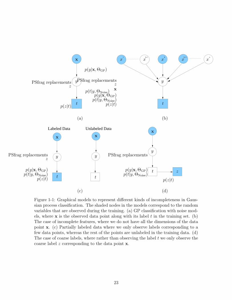
1-1 Graphical models to represent different kinds of incompleteness inGaussian process classification. The shaded nodes in the models corre-spond to the random variables that are observed during the training.(a) GP classification with noise models, where x is the observed datapoint along with its label t in the training set. (b) The case of incom-plete features, where we do not have all the dimensions of the datapoint x. (c) Partially labeled data where we only observe labels cor-responding to a few data points, whereas the rest of the points areunlabeled in the training data. (d) The case of coarse labels, whererather than observing the label t we only observe the coarse label zcorresponding to the data point x. . . . . . . . . . . . . . . . . . . . 23

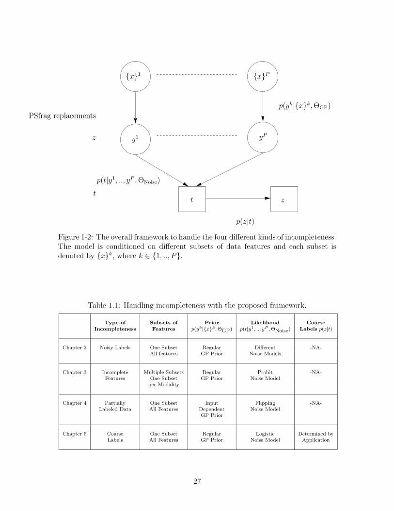
1-2 The overall framework to handle the four different kinds of incomplete-ness. The model is conditioned on different subsets of data featuresand each subset is denoted by {x}k, where k ∈ {1, .., P}. . . . . . . . 27

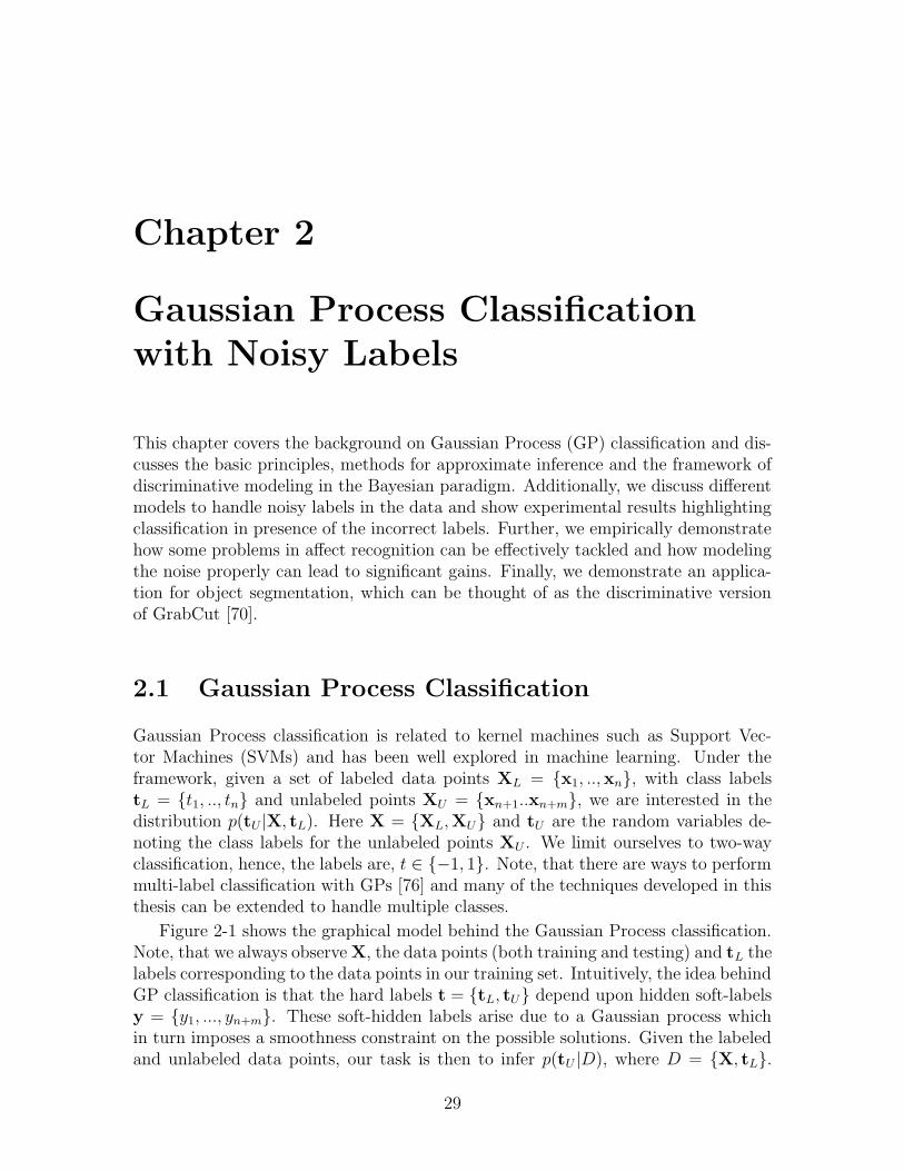
2-1 Graphical model for Gaussian process classification. Note that, X ={XL,XU} and is observed for both training and test data points. Alsot = {tL, tU}; however, only tL corresponding to the labeled data pointsare observed. . . . . . . . . . . . . . . . . . . . . . . . . . . . . . . . 30

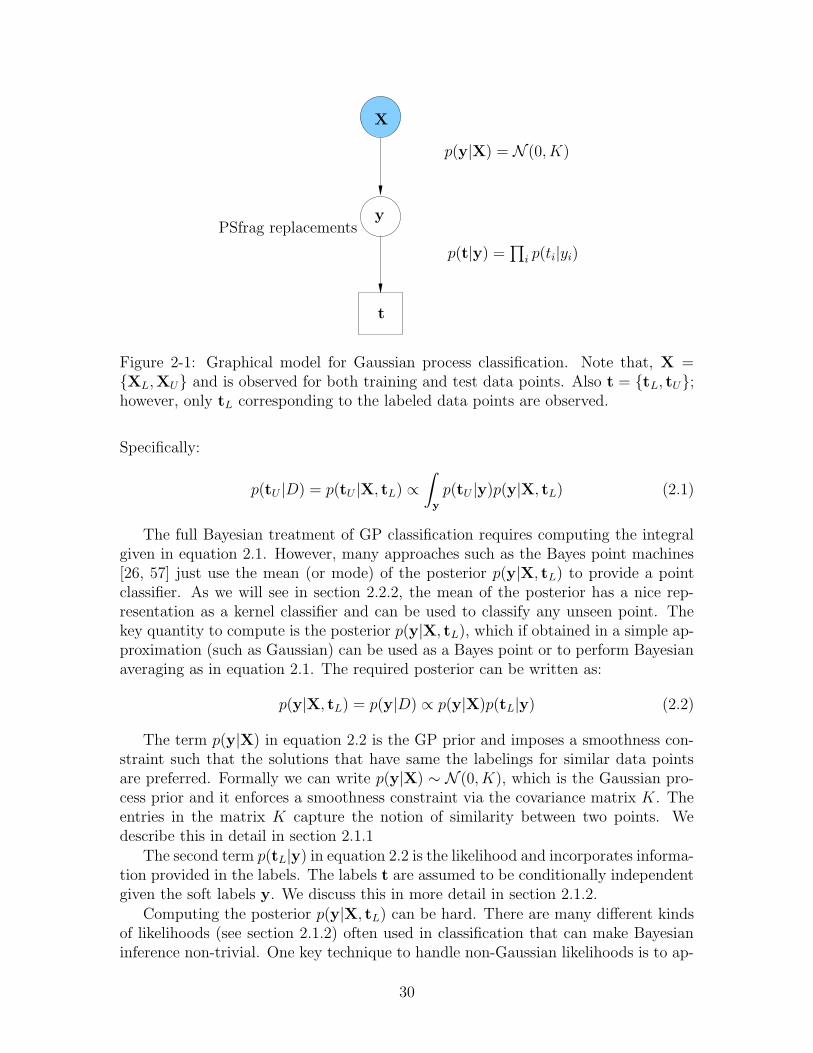
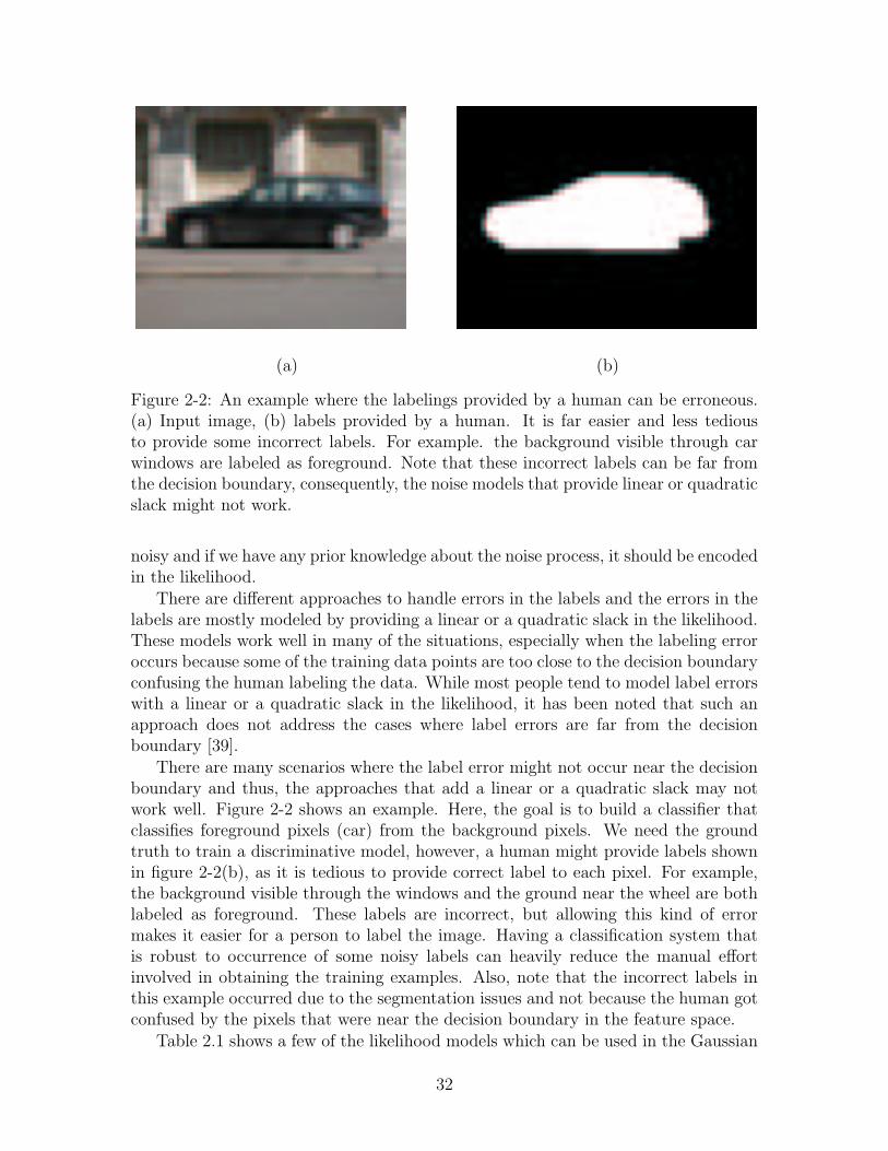
2-2 An example where the labelings provided by a human can be erroneous.(a) Input image, (b) labels provided by a human. It is far easier and lesstedious to provide some incorrect labels. For example. the backgroundvisible through car windows are labeled as foreground. Note that theseincorrect labels can be far from the decision boundary, consequently,the noise models that provide linear or quadratic slack might not work. 32

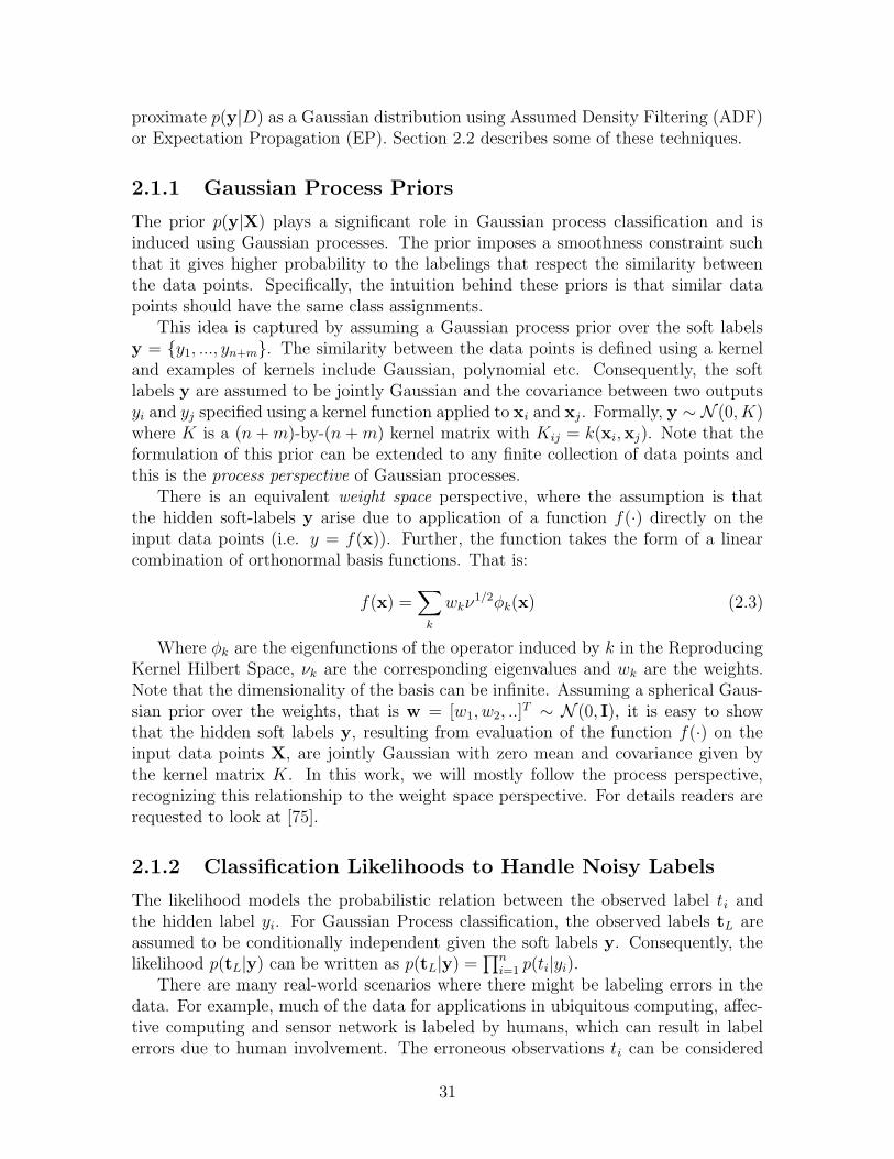
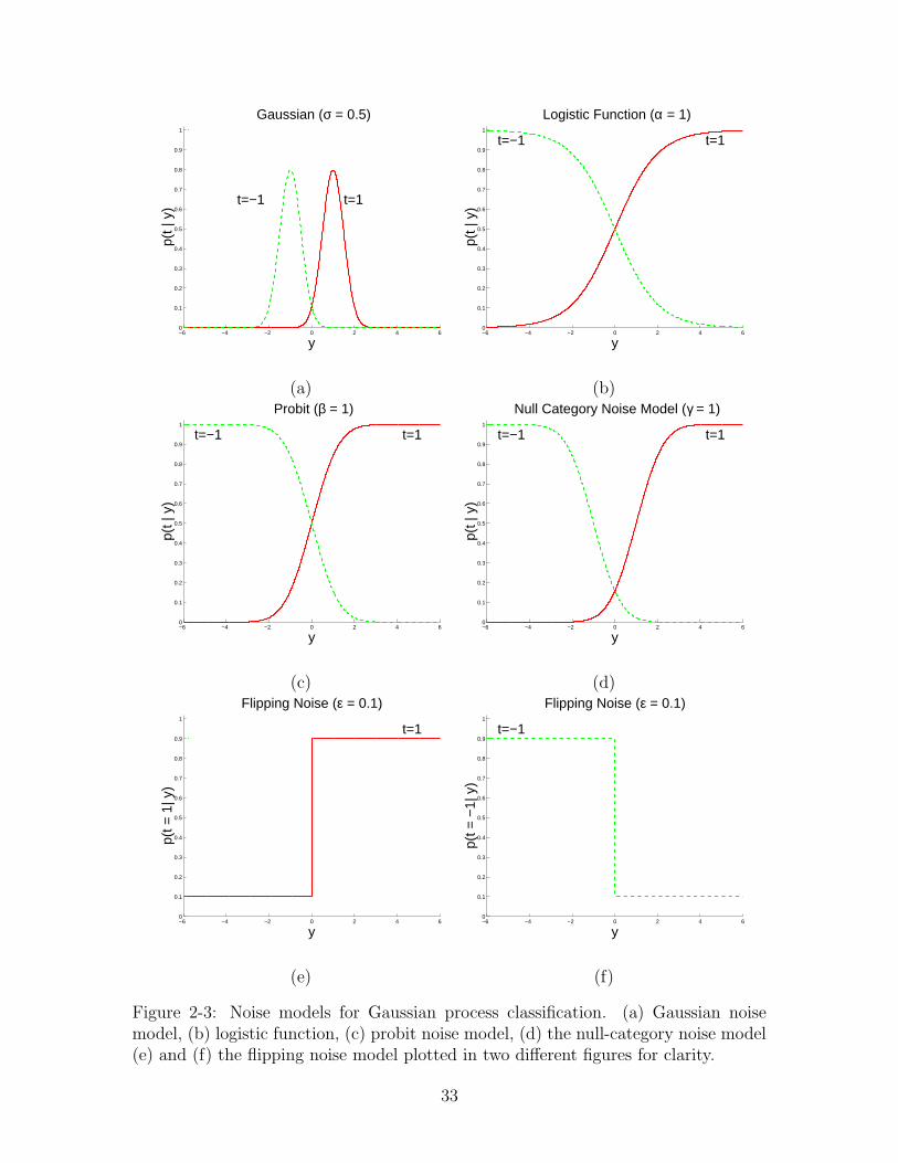
2-3 Noise models for Gaussian process classification. (a) Gaussian noisemodel, (b) logistic function, (c) probit noise model, (d) the null-categorynoise model (e) and (f) the flipping noise model plotted in two differentfigures for clarity. . . . . . . . . . . . . . . . . . . . . . . . . . . . . . 33

2-4 The outline for approximate inference using Expectation Propagationfor Gaussian process classification. . . . . . . . . . . . . . . . . . . . . 37

2-5 The architecture for detecting quitters in learning environments. . . . 41

2-6 Effect of different noise models for Gaussian process classification. (a)Training data with one noisy label. Bayes point classification boundaryusing (b) the probit noise model and (c) the flipping noise model. . . 43

11

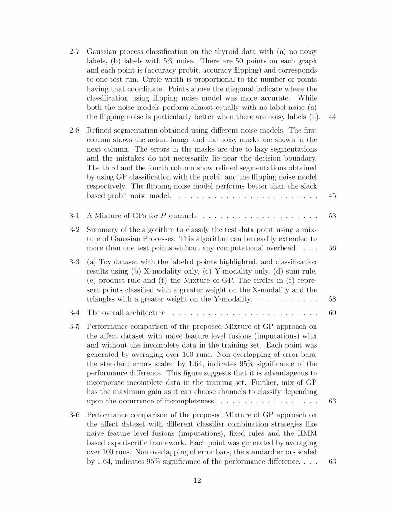
2-7 Gaussian process classification on the thyroid data with (a) no noisylabels, (b) labels with 5% noise. There are 50 points on each graphand each point is (accuracy probit, accuracy flipping) and correspondsto one test run. Circle width is proportional to the number of pointshaving that coordinate. Points above the diagonal indicate where theclassification using flipping noise model was more accurate. Whileboth the noise models perform almost equally with no label noise (a)the flipping noise is particularly better when there are noisy labels (b). 44

2-8 Refined segmentation obtained using different noise models. The firstcolumn shows the actual image and the noisy masks are shown in thenext column. The errors in the masks are due to lazy segmentationsand the mistakes do not necessarily lie near the decision boundary.The third and the fourth column show refined segmentations obtainedby using GP classification with the probit and the flipping noise modelrespectively. The flipping noise model performs better than the slackbased probit noise model. . . . . . . . . . . . . . . . . . . . . . . . . 45

3-1 A Mixture of GPs for P channels . . . . . . . . . . . . . . . . . . . . 53

3-2 Summary of the algorithm to classify the test data point using a mix-ture of Gaussian Processes. This algorithm can be readily extended tomore than one test points without any computational overhead. . . . 56

3-3 (a) Toy dataset with the labeled points highlighted, and classificationresults using (b) X-modality only, (c) Y-modality only, (d) sum rule,(e) product rule and (f) the Mixture of GP. The circles in (f) repre-sent points classified with a greater weight on the X-modality and thetriangles with a greater weight on the Y-modality. . . . . . . . . . . . 58

3-4 The overall architecture . . . . . . . . . . . . . . . . . . . . . . . . . 60

3-5 Performance comparison of the proposed Mixture of GP approach onthe affect dataset with naive feature level fusions (imputations) withand without the incomplete data in the training set. Each point wasgenerated by averaging over 100 runs. Non overlapping of error bars,the standard errors scaled by 1.64, indicates 95% significance of theperformance difference. This figure suggests that it is advantageous toincorporate incomplete data in the training set. Further, mix of GPhas the maximum gain as it can choose channels to classify dependingupon the occurrence of incompleteness. . . . . . . . . . . . . . . . . . 63

3-6 Performance comparison of the proposed Mixture of GP approach onthe affect dataset with different classifier combination strategies likenaive feature level fusions (imputations), fixed rules and the HMMbased expert-critic framework. Each point was generated by averagingover 100 runs. Non overlapping of error bars, the standard errors scaledby 1.64, indicates 95% significance of the performance difference. . . . 63

12

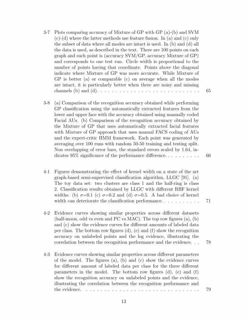
3-7 Plots comparing accuracy of Mixture of GP with GP (a)-(b) and SVM(c)-(d) where the latter methods use feature fusion. In (a) and (c) onlythe subset of data where all modes are intact is used. In (b) and (d) allthe data is used, as described in the text. There are 100 points on eachgraph and each point is (accuracy SVM/GP, accuracy Mixture of GP)and corresponds to one test run. Circle width is proportional to thenumber of points having that coordinate. Points above the diagonalindicate where Mixture of GP was more accurate. While Mixture ofGP is better (a) or comparable (c) on average when all the modesare intact, it is particularly better when there are noisy and missingchannels (b) and (d). . . . . . . . . . . . . . . . . . . . . . . . . . . . 65

3-8 (a) Comparison of the recognition accuracy obtained while performingGP classification using the automatically extracted features from thelower and upper face with the accuracy obtained using manually codedFacial AUs. (b) Comparison of the recognition accuracy obtained bythe Mixture of GP that uses automatically extracted facial featureswith Mixture of GP approach that uses manual FACS coding of AUsand the expert-critic HMM framework. Each point was generated byaveraging over 100 runs with random 50-50 training and testing split.Non overlapping of error bars, the standard errors scaled by 1.64, in-dicates 95% significance of the performance difference. . . . . . . . . . 66

4-1 Figures demonstrating the effect of kernel width on a state of the artgraph-based semi-supervised classification algorithm, LLGC [91]. (a)The toy data set: two clusters are class 1 and the half-ring is class2. Classification results obtained by LLGC with different RBF kernelwidths: (b) σ=0.1 (c) σ=0.2 and (d) σ=0.5. A bad choice of kernelwidth can deteriorate the classification performance. . . . . . . . . . . 71

4-2 Evidence curves showing similar properties across different datasets(half-moon, odd vs even and PC vs MAC). The top row figures (a), (b)and (c) show the evidence curves for different amounts of labeled dataper class. The bottom row figures (d), (e) and (f) show the recognitionaccuracy on unlabeled points and the log evidence, illustrating thecorrelation between the recognition performance and the evidence. . . 78

4-3 Evidence curves showing similar properties across different parametersof the model. The figures (a), (b) and (c) show the evidence curvesfor different amount of labeled data per class for the three differentparameters in the model. The bottom row figures (d), (e) and (f)show the recognition accuracy on unlabeled points and the evidence,illustrating the correlation between the recognition performance andthe evidence. . . . . . . . . . . . . . . . . . . . . . . . . . . . . . . . 79

13

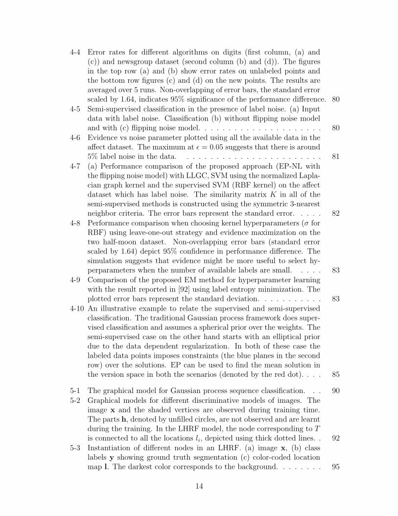
4-4 Error rates for different algorithms on digits (first column, (a) and(c)) and newsgroup dataset (second column (b) and (d)). The figuresin the top row (a) and (b) show error rates on unlabeled points andthe bottom row figures (c) and (d) on the new points. The results areaveraged over 5 runs. Non-overlapping of error bars, the standard errorscaled by 1.64, indicates 95% significance of the performance difference. 80

4-5 Semi-supervised classification in the presence of label noise. (a) Inputdata with label noise. Classification (b) without flipping noise modeland with (c) flipping noise model. . . . . . . . . . . . . . . . . . . . . 80

4-6 Evidence vs noise parameter plotted using all the available data in theaffect dataset. The maximum at ε = 0.05 suggests that there is around5% label noise in the data. . . . . . . . . . . . . . . . . . . . . . . . 81

4-7 (a) Performance comparison of the proposed approach (EP-NL withthe flipping noise model) with LLGC, SVM using the normalized Lapla-cian graph kernel and the supervised SVM (RBF kernel) on the affectdataset which has label noise. The similarity matrix K in all of thesemi-supervised methods is constructed using the symmetric 3-nearestneighbor criteria. The error bars represent the standard error. . . . . 82

4-8 Performance comparison when choosing kernel hyperparameters (σ forRBF) using leave-one-out strategy and evidence maximization on thetwo half-moon dataset. Non-overlapping error bars (standard errorscaled by 1.64) depict 95% confidence in performance difference. Thesimulation suggests that evidence might be more useful to select hy-perparameters when the number of available labels are small. . . . . 83

4-9 Comparison of the proposed EM method for hyperparameter learningwith the result reported in [92] using label entropy minimization. Theplotted error bars represent the standard deviation. . . . . . . . . . . 83

4-10 An illustrative example to relate the supervised and semi-supervisedclassification. The traditional Gaussian process framework does super-vised classification and assumes a spherical prior over the weights. Thesemi-supervised case on the other hand starts with an elliptical priordue to the data dependent regularization. In both of these case thelabeled data points imposes constraints (the blue planes in the secondrow) over the solutions. EP can be used to find the mean solution inthe version space in both the scenarios (denoted by the red dot). . . . 85

5-1 The graphical model for Gaussian process sequence classification. . . 90

5-2 Graphical models for different discriminative models of images. Theimage x and the shaded vertices are observed during training time.The parts h, denoted by unfilled circles, are not observed and are learntduring the training. In the LHRF model, the node corresponding to Tis connected to all the locations li, depicted using thick dotted lines. . 92

5-3 Instantiation of different nodes in an LHRF. (a) image x, (b) classlabels y showing ground truth segmentation (c) color-coded locationmap l. The darkest color corresponds to the background. . . . . . . . 95

14

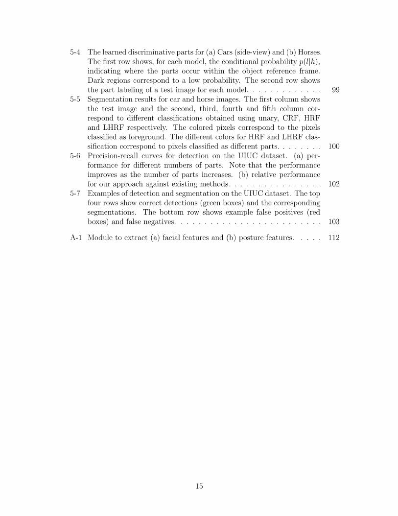
5-4 The learned discriminative parts for (a) Cars (side-view) and (b) Horses.The first row shows, for each model, the conditional probability p(l|h),indicating where the parts occur within the object reference frame.Dark regions correspond to a low probability. The second row showsthe part labeling of a test image for each model. . . . . . . . . . . . . 99

5-5 Segmentation results for car and horse images. The first column showsthe test image and the second, third, fourth and fifth column cor-respond to different classifications obtained using unary, CRF, HRFand LHRF respectively. The colored pixels correspond to the pixelsclassified as foreground. The different colors for HRF and LHRF clas-sification correspond to pixels classified as different parts. . . . . . . . 100

5-6 Precision-recall curves for detection on the UIUC dataset. (a) per-formance for different numbers of parts. Note that the performanceimproves as the number of parts increases. (b) relative performancefor our approach against existing methods. . . . . . . . . . . . . . . . 102

5-7 Examples of detection and segmentation on the UIUC dataset. The topfour rows show correct detections (green boxes) and the correspondingsegmentations. The bottom row shows example false positives (redboxes) and false negatives. . . . . . . . . . . . . . . . . . . . . . . . . 103

A-1 Module to extract (a) facial features and (b) posture features. . . . . 112

15

16

List of Tables

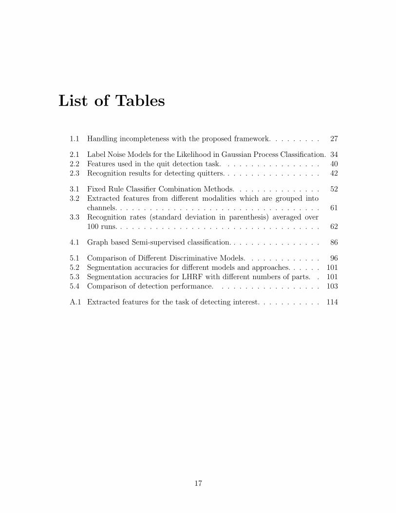
1.1 Handling incompleteness with the proposed framework. . . . . . . . . 27

2.1 Label Noise Models for the Likelihood in Gaussian Process Classification. 342.2 Features used in the quit detection task. . . . . . . . . . . . . . . . . 402.3 Recognition results for detecting quitters. . . . . . . . . . . . . . . . . 42

3.1 Fixed Rule Classifier Combination Methods. . . . . . . . . . . . . . . 523.2 Extracted features from different modalities which are grouped into

channels. . . . . . . . . . . . . . . . . . . . . . . . . . . . . . . . . . . 613.3 Recognition rates (standard deviation in parenthesis) averaged over

100 runs. . . . . . . . . . . . . . . . . . . . . . . . . . . . . . . . . . . 62

4.1 Graph based Semi-supervised classification. . . . . . . . . . . . . . . . 86

5.1 Comparison of Different Discriminative Models. . . . . . . . . . . . . 965.2 Segmentation accuracies for different models and approaches. . . . . . 1015.3 Segmentation accuracies for LHRF with different numbers of parts. . 1015.4 Comparison of detection performance. . . . . . . . . . . . . . . . . . 103

A.1 Extracted features for the task of detecting interest. . . . . . . . . . . 114

17

18

Chapter 1

Introduction

Classification is one of the key tasks in many domains including affective computingand machine perception. For example, consider a computerized affective learningcompanion, a pro-active companion of a child working on an analytic task that aimsto be sensitive to the emotional and cognitive aspects of the learning experience inan unobtrusive way. The affective learning companion [33] needs to reason aboutthe emotional state of the learner based on facial expressions, the posture and othercontext information. The extracted information form the face, the posture and thecontext are called observations, which are sensed through sensors such as a videocamera, a posture sensing chair and other hardware devices or a software. One ofthe main goals of the pattern recognition system is to associate a class-label withdifferent observations, where the class-labels correspond to different affective statessuch as interest, boredom etc. Similarly, there are activity recognition scenarios,where the aim is to recognize different activities happening in the surroundings usinga variety of sensors. For example, using these sensors we can obtain observations thatdescribe the position information using a global positioning system (GPS), status ofthe cellular phone (that is what cell towers are visible), pedometer readings etc. Basedon these observations, the task in an activity recognition scenario can be to identifyactivities, such as driving to the office, sitting, walking home. The same analogy canbe extended to low-level vision tasks such as object detection. Given an image, theobject detection and the segmentation task can be posed as a classification problem,where the aim is to classify each individual pixel as a background or a part belongingto the foreground. The observations in all of these scenarios are multi-dimensionaland each dimension is considered as a feature. Note, that different modalities, suchas face, posture etc contribute to many features in the observations.

Traditional models of supervised classification aim to learn a decision boundarygiven a set of observations, X = {x1, ..,xn}, and the corresponding class labels,t = {t1, ..tn}. However, there are many scenarios that far exceed this simplisticmodel. Often the training data is plagued by incompleteness: there is only partialinformation available about the observations (incompleteness in X) or about the labels(incompleteness in t).

There are many scenarios that can result in incomplete data. For example, manyapplications in affect recognition, activity recognition and machine perception can

19

encounter incompleteness in observations X, especially where multimodal informationis used, and where information from multiple sensors needs to be fused to recover thevariable of interest. Some of the hardware and algorithms associated with some of themodes might fail occasionally, leading to missing features and making the standardpattern recognition machinery unusable on that chunk of data. Similarly there aremany scenarios which can result in incompleteness in the labels t. For instance, manypractical applications have the characteristic of having very little labeled trainingdata. They usually have lots of data (e.g. video), but most of it is unlabeled (becauseit is tedious, costly, and error-prone to have people label it). Further, the problembecomes even more challenging when there is labeling noise; that is, some data pointshave incorrect labels. Note that the noisy labels can be considered as a special caseof incompleteness, where we only observe a transformed version of the true label. Inmany applications like emotion recognition, there is usually some uncertainty aboutthe true labels of the data; thus, a principled approach is required to handle anylabeling noise in the data. Another case of incompleteness occurs when the datapoints are categorized into easy to label high level classes, instead of much harder toobtain labels of interest. In these scenarios the actual labels of interest might be hardor very expensive to obtain and usually it is much easier and quicker to obtain coarseror auxiliary labels that co-occur with the labels of interest. For instance, in activityrecognition it is usually very tiresome to collect labels corresponding to individuallow-level activities such as walking, sleeping etc. However, it is quicker and far moreconvenient to obtain labels that describe your location (for example, outdoors vs.indoors).

Traditionally incompleteness has been addressed in a generative framework, whichaims to jointly model the observations X together with the labels t and where the in-completeness is treated as a hidden or a latent variable. These generative approacheslearn by integrating or marginalizing over the incompleteness. However, the genera-tive approaches can run into problems when the dimensionality of observations is largeor when there are very few samples in the training data; thus, making it impossibleto learn the underlying probability distribution of the observations.

On the other hand, the discriminative approaches model the distribution of thelabels conditioned on the observations; thus, the distribution of the input data Xis never explicitly modeled. This alleviates some of the problems encountered withthe generative model; however, now it becomes non-trivial to extend the frameworkto handle incomplete data. Some of the recent successes of discriminative modelsover generative models makes a strong case to develop methods that can handleincompleteness in the discriminative setting.

1.1 Types of Incompleteness

This thesis addresses four different types of incompleteness:

• Incomplete Features: This kind of incompleteness results when there areobservations xi ∈ X with some features unobserved or missing. One example

20

where this kind of incompleteness might occur is multimodal pattern classifi-cation. There are a growing number of scenarios in affective computing andactivity recognition where multimodal information is used. However, the sen-sors might often fail and result in missing or bad data, a frequent problem inmany multimodal systems.

• Partially Labeled Data: Often in affect and activity recognition scenarios itmight be expensive or difficult to obtain the labels. This problem is addressedin semi-supervised classification, where only a part of the available data is an-notated. Specifically, given a set of data points, among which few are labeled,the goal in semi-supervised learning is to predict the labels of the unlabeledpoints using the complete set of data points. By looking at both the labeledand the unlabeled data, the learning algorithm can exploit the distribution ofdata points to learn the classification boundary.

• Coarse Labels: In most activity recognition scenarios, each activity can bebroken down into sub-activities, which often form a hierarchy. Also, in manycases it is easier to build robust classifiers to recognize sub-activities lower inthis hierarchy. Similarly in object recognition from static images, the objectscan be broken down into parts and often it is easier to build robust partsclassifiers than a single object detector. Further, in affect recognition scenariosit is often easier to get high level labels for emotions such as positive/negative orexcited/calm instead of labels such as interest/frustration/surprise. However,fully supervised training of these hierarchical activity/object/affect recognitionsystem is difficult as it is very expensive to obtain training data annotated forall the sub-classes. Also, note that in many scenarios it might be unclear howto select these sub-classes. Thus, the training data might be just annotated forthe higher level classes and the challenge with this kind of data is to train apattern recognition system that exploits the hierarchical structure using onlythe available coarse or auxiliary labelings.

• Noisy Labels: Finally, the machine learning system needs labeled data andthere are many scenarios where the labels provided might be incorrect. Forexample in the domain of affect recognition, getting the ground truth of labelsin natural data is a challenging task. There is always some uncertainty aboutthe true labels of the data. There might be labeling noise; that is, some datapoints might have incorrect labels. We wish to develop a principled approachto handle this type of incompleteness as well as all the other types mentionedabove

1.1.1 Other Types of Incompleteness

The kinds of incompleteness are not limited to the ones described in the previoussection. For example, multiple instance learning [19], solves a different kind of in-completeness where labels are provided to a collection of observations instead of eachindividual observation. Further, the labels in multiple instance learning just indicate

21

whether there is at least one observation in the collection with the label of interest.Thus, multiple instance learning is very different from the kinds of incompleteness de-scribed earlier and is mostly used in applications such as information retrieval. In ourwork we focus mainly on the problems arising in affective computing, activity recog-nition and other machine perception tasks and these applications mostly encounterthe four kinds of incompleteness handled in this document.

1.2 Contributions of the Thesis

This thesis provides a Bayesian framework for learning discriminative models withincomplete data. The framework extends many different approaches to handle differ-ent kinds of incompleteness and provides insights and connections to many existingmethods in semi-supervised learning, sensor-fusion and discriminative modeling. Onemajor advantage of viewing different methods in a single Bayesian framework is thatfirst we can use the Bayesian framework to perform model selection tasks, which werenon-trivial earlier. Second, we can now derive new methods for discriminative model-ing, such as semi-supervised learning and sensor-fusion by exploiting the modularityin the proposed unified framework.

The highly challenging problem addressed in this work is motivated by real-worldproblems in affective computing, activity recognition and machine perception andincludes the scenarios described above: there is often multi-sensory data, channelsare frequently missing, most of the training data is unlabeled, there might be labelingerrors in the data and the available labels might be only loosely related to the desiredones. We present a Bayesian framework that extends the discriminative paradigmof classification to handle these four types of incompleteness. The framework buildsupon Gaussian process classification and the learning and inference in this class ofmodels is performed using a variety of Bayesian inference techniques, like ExpectationPropagation [56], variational approximate inference and Monte-Carlo.

Figure 1-1 graphically depicts the Gaussian process classification and the differentcases of incompleteness. The GP classification is a Bayesian framework for discrimi-native modeling and the aim is to model the distribution of the labels conditioned onthe data points. The model assumes hidden real-valued random variable y that im-poses a smoothness constraint on the solution via a Gaussian process with parametersΘGP (denoted by p(y|x,ΘGP) in figure 1-1(a)). The relationship between the hiddenrandom variable y and the observed label t is captured by the term p(t|y,ΘNoise) andcan be used to encode the noise process to handle noisy labels. Figures 1-1(b), (c)and (d) show the rest of the cases of incompleteness. In figure 1-1(d) the distribu-tion p(t, z) models the relationship between the label t and the coarse label z. TheGP classification framework has the capability to express the different scenarios ofincompleteness and our aim in this thesis is to exploit the flexibility of the Bayesianframework to handle incomplete data in the discriminative setting. The followingbriefly describes the basic principles of the approach derived in this thesis:

• Incomplete Features: The incompleteness in features is addressed using amixture of Gaussian processes [32]. The idea is to first train multiple classifiers

22

PSfrag replacementsz

y

x

t

p(y|x,ΘGP)

p(t|y,ΘNoise)

p(z|t)

k1 k-1 k+1 n

PSfrag replacementsz

y

x

t

p(y|x,ΘGP)p(t|y,ΘNoise)

p(z|t)

xxxx x

(a) (b)

Labeled Data Unlabeled Data

PSfrag replacementsz

yy

xx

tt

p(y|x,ΘGP)p(t|y,ΘNoise)

p(z|t)

PSfrag replacements

z

y

x

tp(y|x,ΘGP)p(t|y,ΘNoise)

p(z|t)

(c) (d)

Figure 1-1: Graphical models to represent different kinds of incompleteness in Gaus-sian process classification. The shaded nodes in the models correspond to the randomvariables that are observed during the training. (a) GP classification with noise mod-els, where x is the observed data point along with its label t in the training set. (b)The case of incomplete features, where we do not have all the dimensions of the datapoint x. (c) Partially labeled data where we only observe labels corresponding to afew data points, whereas the rest of the points are unlabeled in the training data. (d)The case of coarse labels, where rather than observing the label t we only observe thecoarse label z corresponding to the data point x.

23

based on different subsets of features and then combine decisions from thesemultiple classifiers depending upon what channels are missing or erroneous.The framework extends the Gaussian Process classification to the mixture ofGaussian Processes, where the classification using each channel is learned viaExpectation Propagation (EP), a technique for approximate Bayesian inference.The resulting posterior over each classification function is a product of Gaus-sians and can be updated very quickly. We evaluate the multi-sensor classifica-tion scheme on the challenging task of detecting the affective state of interestin children trying to solve a puzzle, combining sensory information from theface, the postures and the state of the puzzle task, to infer the student’s state.The proposed unified approach achieves a significantly better recognition accu-racy than classification based on individual channels and the standard classifiercombination methods.

• Partially Labeled Data: The incompleteness due to partially labeled datais handled using input-dependent regularization [74]. The proposed Bayesianframework is an extension of the Gaussian Process classification and connectsmany recent graph-based semi-supervised learning work [79, 91, 92, 94]. We useExpectation Propagation that provides better approximations than previouslyused Laplace [94], with an additional benefit of deriving an algorithm that learnsthe kernel and the hyperparameters for graph based semi-supervised classifica-tion methods, while adhering to a Bayesian framework. An algorithm based onExpectation Maximization (EM) is used to maximize the evidence for simulta-neously tuning the hyperparameters that define the structure of the similaritygraph, the parameters that determine the transformation of the graph Lapla-cian, and any other parameters of the model. An additional advantage of theBayesian framework is that we can explicitly model and estimate the differenttypes of label noise in the data.

• Coarse Labels: The case of coarse label can be solved using the techniquesthat are used in generative modeling and have been earlier explored in analysisof hand-written diagrams using hidden random fields (HRF) [81]. Specifically,since we explicitly model the distribution of labels conditioned on X, we canmarginalize over the hidden variables that correspond to unknown but desiredlabels. The advantage of modeling sub-activities discriminatively is that theirrelevant sources of variability do not need to be modeled, whereas the gen-erative alternative has to allow for all sources of variability in the data. Onekey contribution of the work mentioned in this thesis is the extension of HRFto model long range spatial dependencies. These models are specially effectiveon computer vision tasks and we use the proposed framework to address theproblem of part-based object detection and recognition. By introducing theglobal position of the object as a latent variable, we can model the long-rangespatial configuration of parts, as well as their local interactions. Experimentson benchmark datasets show that the use of discriminative parts leads to state-of-the-art detection and segmentation performance, with the additional benefit

24

of obtaining a labeling of the object’s component parts.

• Noisy Labels: We propose to handle the noise in the data by using differentkinds of noise models that allow different kinds of errors. The challenge here is tochoose a good model that agrees with the training data. One of the advantagesof this Bayesian framework is that we can use evidence maximization criteriato select the noise model and its parameters.

Figure 1-2 shows the overall framework to handle different kinds of incompleteness.The model is conditioned on different subsets of features denoted by {x}k in the figure.The model assumes that the hidden soft labels yk arise due to a Gaussian processconditioned on the subset of features. The label of interest is denoted by t and zis the coarse label. Depending upon the kind of incompleteness, different randomvariable are observed during the training time (see figure 1-1). Further, the model ischaracterized using p(yk|{x}k,ΘGP), p(t|y1, .., yP ,ΘNoise) and p(z|t) corresponding tothe smoothness constraint (parameterized by ΘGP), the noise model (parameterizedby ΘNoise) and the statistical relationship between the label and the coarse labelrespectively. All the solutions proposed in this thesis can be combined into a singleframework by considering different choices of these quantities and the different subsetsof the features. Table 1.1 depicts these choices and highlights the relationship to theoverall framework.

1.3 Thesis Outline

The chapters of the thesis are organized as follows:

• Chapter 2: Gaussian Process Classification with Noisy Labels

Gaussian Process classification, which is the basic building block of the thesisis reviewed. Learning with noisy labels is addressed and a number of differentnoise models are discussed. Further, we demonstrate how various techniques forGaussian process classification can be exploited to solve the challenging problemof affect recognition and object segmentation when only the noisy masks areavailable.

• Chapter 3: Mixture of Gaussian Processes to Combine Multiple Modalities

The incompleteness due to missing channels and features is addressed in thischapter and we specifically focus on when there is limited labeled data available.The mixture of Gaussian Process classifiers is introduced and an approximateinference procedure for joint training is proposed, which results in a frameworkcapable of quickly re-learning the classification given updated label associations.

• Chapter 4: Gaussian Process Classification with Partially Labeled Data

This chapter discusses how the basic Gaussian Process classification frameworkcan be extended to semi-supervised classification. The proposed framework

25

exploits input dependent regularization to handle the incompleteness arisingdue to partially labeled data and has connections to recently proposed graphbased semi-supervised classification.

• Chapter 5: Located Hidden Random Fields to Learn Discriminative Parts

This chapter extends the discriminative paradigm of classification to handlecoarse and auxiliary labels. Rather than using the generative paradigm wherethe model tries to explain all the variability in the data, the focus here is onlearning sub-classes discriminatively; thus, ultimately helping in explaining theprovided coarse labels well.

• Chapter 6: Conclusion and Future Work

This chapter summarizes the contributions and concludes the thesis by propos-ing extensions and future work.

26

PSfrag replacements

z

z y1 yP

{x}1 {x}P

tt

p(yk|{x}k,ΘGP)

p(t|y1, .., yP ,ΘNoise)

p(z|t)

Figure 1-2: The overall framework to handle the four different kinds of incompleteness.The model is conditioned on different subsets of data features and each subset isdenoted by {x}k, where k ∈ {1, .., P}.

Table 1.1: Handling incompleteness with the proposed framework.

Type of Subsets of Prior Likelihood Coarse

Incompleteness Features p(yk|{x}k, ΘGP) p(t|y1, .., yP , ΘNoise) Labels p(z|t)

Chapter 2 Noisy Labels One Subset Regular Different -NA-All features GP Prior Noise Models

Chapter 3 Incomplete Multiple Subsets Regular Probit -NA-Features One Subset GP Prior Noise Model

per Modality

Chapter 4 Partially One Subset Input Flipping -NA-Labeled Data All Features Dependent Noise Model

GP Prior

Chapter 5 Coarse One Subset Regular Logistic Determined byLabels All Features GP Prior Noise Model Application

27

28

Chapter 2

Gaussian Process Classificationwith Noisy Labels

This chapter covers the background on Gaussian Process (GP) classification and dis-cusses the basic principles, methods for approximate inference and the framework ofdiscriminative modeling in the Bayesian paradigm. Additionally, we discuss differentmodels to handle noisy labels in the data and show experimental results highlightingclassification in presence of the incorrect labels. Further, we empirically demonstratehow some problems in affect recognition can be effectively tackled and how modelingthe noise properly can lead to significant gains. Finally, we demonstrate an applica-tion for object segmentation, which can be thought of as the discriminative versionof GrabCut [70].

2.1 Gaussian Process Classification

Gaussian Process classification is related to kernel machines such as Support Vec-tor Machines (SVMs) and has been well explored in machine learning. Under theframework, given a set of labeled data points XL = {x1, ..,xn}, with class labelstL = {t1, .., tn} and unlabeled points XU = {xn+1..xn+m}, we are interested in thedistribution p(tU |X, tL). Here X = {XL,XU} and tU are the random variables de-noting the class labels for the unlabeled points XU . We limit ourselves to two-wayclassification, hence, the labels are, t ∈ {−1, 1}. Note, that there are ways to performmulti-label classification with GPs [76] and many of the techniques developed in thisthesis can be extended to handle multiple classes.

Figure 2-1 shows the graphical model behind the Gaussian Process classification.Note, that we always observe X, the data points (both training and testing) and tL thelabels corresponding to the data points in our training set. Intuitively, the idea behindGP classification is that the hard labels t = {tL, tU} depend upon hidden soft-labelsy = {y1, ..., yn+m}. These soft-hidden labels arise due to a Gaussian process whichin turn imposes a smoothness constraint on the possible solutions. Given the labeledand unlabeled data points, our task is then to infer p(tU |D), where D = {X, tL}.

29

PSfrag replacementsy

X

t

p(y|X) = N (0, K)

p(t|y) =∏

i p(ti|yi)

Figure 2-1: Graphical model for Gaussian process classification. Note that, X ={XL,XU} and is observed for both training and test data points. Also t = {tL, tU};however, only tL corresponding to the labeled data points are observed.

Specifically:

p(tU |D) = p(tU |X, tL) ∝

∫

y

p(tU |y)p(y|X, tL) (2.1)

The full Bayesian treatment of GP classification requires computing the integralgiven in equation 2.1. However, many approaches such as the Bayes point machines[26, 57] just use the mean (or mode) of the posterior p(y|X, tL) to provide a pointclassifier. As we will see in section 2.2.2, the mean of the posterior has a nice rep-resentation as a kernel classifier and can be used to classify any unseen point. Thekey quantity to compute is the posterior p(y|X, tL), which if obtained in a simple ap-proximation (such as Gaussian) can be used as a Bayes point or to perform Bayesianaveraging as in equation 2.1. The required posterior can be written as:

p(y|X, tL) = p(y|D) ∝ p(y|X)p(tL|y) (2.2)

The term p(y|X) in equation 2.2 is the GP prior and imposes a smoothness con-straint such that the solutions that have same the labelings for similar data pointsare preferred. Formally we can write p(y|X) ∼ N (0, K), which is the Gaussian pro-cess prior and it enforces a smoothness constraint via the covariance matrix K. Theentries in the matrix K capture the notion of similarity between two points. Wedescribe this in detail in section 2.1.1

The second term p(tL|y) in equation 2.2 is the likelihood and incorporates informa-tion provided in the labels. The labels t are assumed to be conditionally independentgiven the soft labels y. We discuss this in more detail in section 2.1.2.

Computing the posterior p(y|X, tL) can be hard. There are many different kindsof likelihoods (see section 2.1.2) often used in classification that can make Bayesianinference non-trivial. One key technique to handle non-Gaussian likelihoods is to ap-

30

proximate p(y|D) as a Gaussian distribution using Assumed Density Filtering (ADF)or Expectation Propagation (EP). Section 2.2 describes some of these techniques.

2.1.1 Gaussian Process Priors

The prior p(y|X) plays a significant role in Gaussian process classification and isinduced using Gaussian processes. The prior imposes a smoothness constraint suchthat it gives higher probability to the labelings that respect the similarity betweenthe data points. Specifically, the intuition behind these priors is that similar datapoints should have the same class assignments.

This idea is captured by assuming a Gaussian process prior over the soft labelsy = {y1, ..., yn+m}. The similarity between the data points is defined using a kerneland examples of kernels include Gaussian, polynomial etc. Consequently, the softlabels y are assumed to be jointly Gaussian and the covariance between two outputsyi and yj specified using a kernel function applied to xi and xj. Formally, y ∼ N (0, K)where K is a (n +m)-by-(n +m) kernel matrix with Kij = k(xi,xj). Note that theformulation of this prior can be extended to any finite collection of data points andthis is the process perspective of Gaussian processes.

There is an equivalent weight space perspective, where the assumption is thatthe hidden soft-labels y arise due to application of a function f(·) directly on theinput data points (i.e. y = f(x)). Further, the function takes the form of a linearcombination of orthonormal basis functions. That is:

f(x) =∑

k

wkν1/2φk(x) (2.3)

Where φk are the eigenfunctions of the operator induced by k in the ReproducingKernel Hilbert Space, νk are the corresponding eigenvalues and wk are the weights.Note that the dimensionality of the basis can be infinite. Assuming a spherical Gaus-sian prior over the weights, that is w = [w1, w2, ..]

T ∼ N (0, I), it is easy to showthat the hidden soft labels y, resulting from evaluation of the function f(·) on theinput data points X, are jointly Gaussian with zero mean and covariance given bythe kernel matrix K. In this work, we will mostly follow the process perspective,recognizing this relationship to the weight space perspective. For details readers arerequested to look at [75].

2.1.2 Classification Likelihoods to Handle Noisy Labels

The likelihood models the probabilistic relation between the observed label ti andthe hidden label yi. For Gaussian Process classification, the observed labels tL areassumed to be conditionally independent given the soft labels y. Consequently, thelikelihood p(tL|y) can be written as p(tL|y) =

∏ni=1 p(ti|yi).

There are many real-world scenarios where there might be labeling errors in thedata. For example, much of the data for applications in ubiquitous computing, affec-tive computing and sensor network is labeled by humans, which can result in labelerrors due to human involvement. The erroneous observations ti can be considered

31

(a) (b)

Figure 2-2: An example where the labelings provided by a human can be erroneous.(a) Input image, (b) labels provided by a human. It is far easier and less tediousto provide some incorrect labels. For example. the background visible through carwindows are labeled as foreground. Note that these incorrect labels can be far fromthe decision boundary, consequently, the noise models that provide linear or quadraticslack might not work.

noisy and if we have any prior knowledge about the noise process, it should be encodedin the likelihood.

There are different approaches to handle errors in the labels and the errors in thelabels are mostly modeled by providing a linear or a quadratic slack in the likelihood.These models work well in many of the situations, especially when the labeling erroroccurs because some of the training data points are too close to the decision boundaryconfusing the human labeling the data. While most people tend to model label errorswith a linear or a quadratic slack in the likelihood, it has been noted that such anapproach does not address the cases where label errors are far from the decisionboundary [39].

There are many scenarios where the label error might not occur near the decisionboundary and thus, the approaches that add a linear or a quadratic slack may notwork well. Figure 2-2 shows an example. Here, the goal is to build a classifier thatclassifies foreground pixels (car) from the background pixels. We need the groundtruth to train a discriminative model, however, a human might provide labels shownin figure 2-2(b), as it is tedious to provide correct label to each pixel. For example,the background visible through the windows and the ground near the wheel are bothlabeled as foreground. These labels are incorrect, but allowing this kind of errormakes it easier for a person to label the image. Having a classification system thatis robust to occurrence of some noisy labels can heavily reduce the manual effortinvolved in obtaining the training examples. Also, note that the incorrect labels inthis example occurred due to the segmentation issues and not because the human gotconfused by the pixels that were near the decision boundary in the feature space.

Table 2.1 shows a few of the likelihood models which can be used in the Gaussian

32

−6 −4 −2 0 2 4 60

0.1

0.2

0.3

0.4

0.5

0.6

0.7

0.8

0.9

1

Gaussian (σ = 0.5)

t=−1 t=1

p(t |

y)

y−6 −4 −2 0 2 4 60

0.1

0.2

0.3

0.4

0.5

0.6

0.7

0.8

0.9

1

Logistic Function (α = 1)

t=−1 t=1

p(t |

y)

y

(a) (b)

−6 −4 −2 0 2 4 60

0.1

0.2

0.3

0.4

0.5

0.6

0.7

0.8

0.9

1

Probit (β = 1)

t=−1 t=1

p(t |

y)

y−6 −4 −2 0 2 4 60

0.1

0.2

0.3

0.4

0.5

0.6

0.7

0.8

0.9

1

Null Category Noise Model (γ = 1)

t=−1 t=1

p(t |

y)

y

(c) (d)

−6 −4 −2 0 2 4 60

0.1

0.2

0.3

0.4

0.5

0.6

0.7

0.8

0.9

1

Flipping Noise (ε = 0.1)

t=1

p(t =

1| y

)

y−6 −4 −2 0 2 4 60

0.1

0.2

0.3

0.4

0.5

0.6

0.7

0.8

0.9

1

Flipping Noise (ε = 0.1)

t=−1

p(t =

−1|

y)

y

(e) (f)

Figure 2-3: Noise models for Gaussian process classification. (a) Gaussian noisemodel, (b) logistic function, (c) probit noise model, (d) the null-category noise model(e) and (f) the flipping noise model plotted in two different figures for clarity.

33

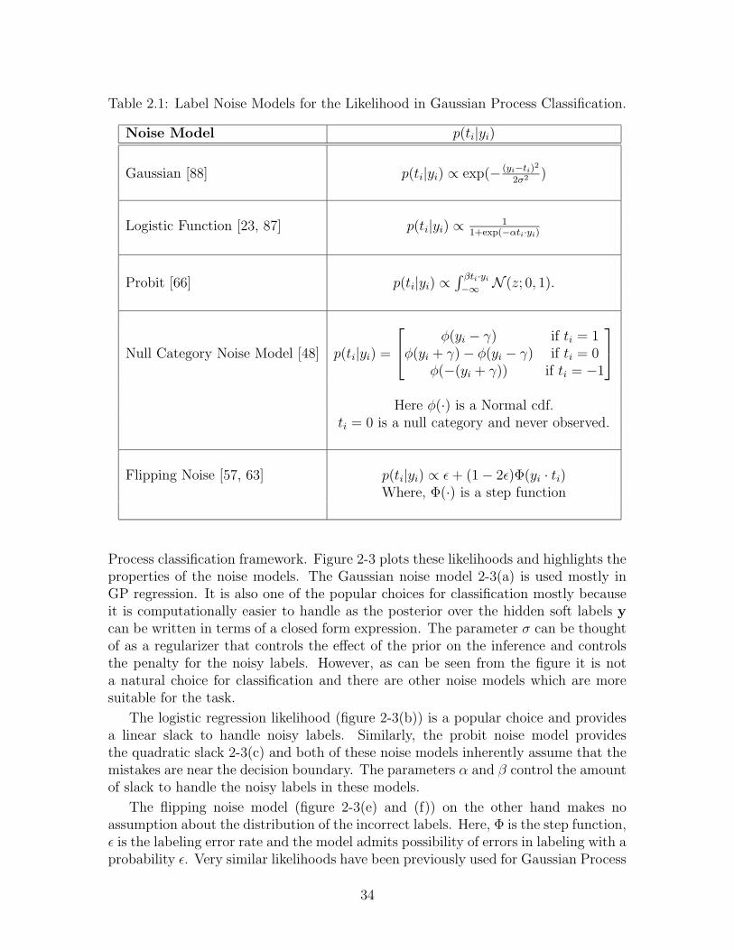
Table 2.1: Label Noise Models for the Likelihood in Gaussian Process Classification.

Noise Model p(ti|yi)

Gaussian [88] p(ti|yi) ∝ exp(− (yi−ti)2

2σ2 )

Logistic Function [23, 87] p(ti|yi) ∝1

1+exp(−αti·yi)

Probit [66] p(ti|yi) ∝∫ βti·yi

−∞N (z; 0, 1).

Null Category Noise Model [48] p(ti|yi) =

φ(yi − γ) if ti = 1φ(yi + γ) − φ(yi − γ) if ti = 0

φ(−(yi + γ)) if ti = −1

Here φ(·) is a Normal cdf.ti = 0 is a null category and never observed.

Flipping Noise [57, 63] p(ti|yi) ∝ ε+ (1 − 2ε)Φ(yi · ti)Where, Φ(·) is a step function

Process classification framework. Figure 2-3 plots these likelihoods and highlights theproperties of the noise models. The Gaussian noise model 2-3(a) is used mostly inGP regression. It is also one of the popular choices for classification mostly becauseit is computationally easier to handle as the posterior over the hidden soft labels ycan be written in terms of a closed form expression. The parameter σ can be thoughtof as a regularizer that controls the effect of the prior on the inference and controlsthe penalty for the noisy labels. However, as can be seen from the figure it is nota natural choice for classification and there are other noise models which are moresuitable for the task.

The logistic regression likelihood (figure 2-3(b)) is a popular choice and providesa linear slack to handle noisy labels. Similarly, the probit noise model providesthe quadratic slack 2-3(c) and both of these noise models inherently assume that themistakes are near the decision boundary. The parameters α and β control the amountof slack to handle the noisy labels in these models.

The flipping noise model (figure 2-3(e) and (f)) on the other hand makes noassumption about the distribution of the incorrect labels. Here, Φ is the step function,ε is the labeling error rate and the model admits possibility of errors in labeling with aprobability ε. Very similar likelihoods have been previously used for Gaussian Process

34

classification [63] and Bayes-point machines [56]. The above described likelihoodexplicitly models the labeling error rate; thus, the model is robust to label noise evenif the mistakes are far from the decision boundary. However, the likelihood function isdiscontinuous; thus, it can cause problems when using optimization techniques suchas gradient descent.

Recently, Lawrence and Jordan [48] introduced the null category noise model (fig-ure 2-3(d)) that tries to imitate the SVM hinge loss function. The biggest advantageof this model appears to be in the semi-supervised cases (see chapter 4). Similar tothe spirit of the SVM the likelihood also assumes that the label errors occur near thedecision boundary.

Except for the case of the Gaussian likelihood, computing the posterior p(y|D) isnon-trivial. The next section discusses how to use approximate inference techniquesto perform GP classification with non-Gaussian likelihoods.

2.2 Approximate Bayesian Inference

As mentioned earlier, the key step in Gaussian process classification is to evaluatethe posterior p(y|D) ∝ p(y|X)p(tL|y). Although the prior p(y|X) is a Gaussiandistribution, the exact posterior may not be a Gaussian and depends on the form ofp(tL|y).

When the noise model is Gaussian, the posterior is just a product of Gaussianterms and has a closed form expression. However, for all other non Gaussian likeli-hoods we have to resort to approximate inference techniques.

There have been a number of approaches for approximate inference for Gaussianprocess classification. There are sampling based techniques such as Markov ChainMonte Carlo and the billiard algorithm [72, 26], which resembles Gibbs sampling. Thesampling based methods can provide very good approximations to the posteriors; how-ever, they are computationally expensive. The deterministic approximation methodson the other hand can be faster and examples include variational approximations,Expectation Propagation, assumed density filtering and the Laplace approximation.Gibbs and Mackay [23] have described how to perform Gaussian process classifica-tion using the variational bounds and similarly, Opper and Winther have used themean field approximation [63]. Another choice is the Laplace approximation, wherethe idea is to use a Taylor series expansion around the mode of the exact posteriorto fit a Gaussian distribution. Assumed density filtering (ADF) and EP, which isa generalization of ADF, have been the most popular methods for deterministic ap-proximate inference in Gaussian process classification [56, 47, 51]. Recently, Kuss andRasmussen [45] compared the Laplace approximation with EP for Gaussian processclassification and the results indicate that EP provides much better approximationsof the posterior. In this thesis we use EP for approximate Bayesian inference forGaussian process classification and the next subsection describes the main principlesbehind the method.

35

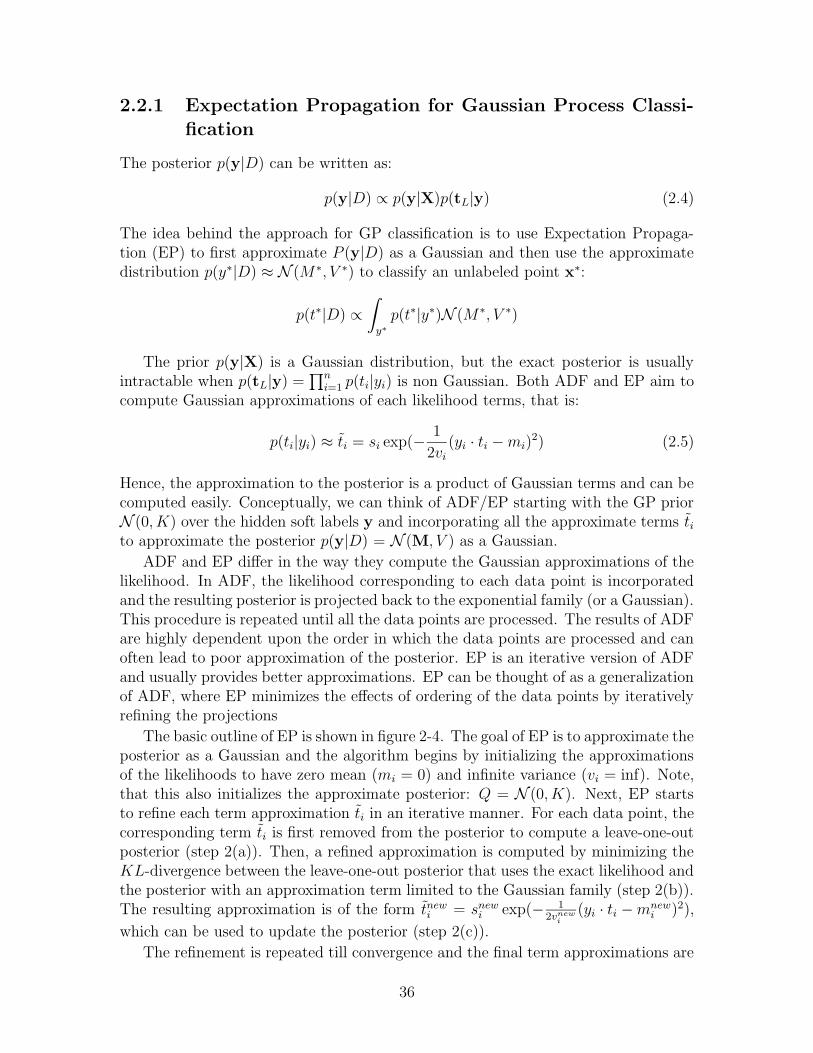
2.2.1 Expectation Propagation for Gaussian Process Classi-fication

The posterior p(y|D) can be written as:

p(y|D) ∝ p(y|X)p(tL|y) (2.4)

The idea behind the approach for GP classification is to use Expectation Propaga-tion (EP) to first approximate P (y|D) as a Gaussian and then use the approximatedistribution p(y∗|D) ≈ N (M ∗, V ∗) to classify an unlabeled point x∗:

p(t∗|D) ∝

∫

y∗

p(t∗|y∗)N (M ∗, V ∗)

The prior p(y|X) is a Gaussian distribution, but the exact posterior is usuallyintractable when p(tL|y) =

∏ni=1 p(ti|yi) is non Gaussian. Both ADF and EP aim to

compute Gaussian approximations of each likelihood terms, that is:

p(ti|yi) ≈ ti = si exp(−1

2vi

(yi · ti −mi)2) (2.5)

Hence, the approximation to the posterior is a product of Gaussian terms and can becomputed easily. Conceptually, we can think of ADF/EP starting with the GP priorN (0, K) over the hidden soft labels y and incorporating all the approximate terms tito approximate the posterior p(y|D) = N (M, V ) as a Gaussian.

ADF and EP differ in the way they compute the Gaussian approximations of thelikelihood. In ADF, the likelihood corresponding to each data point is incorporatedand the resulting posterior is projected back to the exponential family (or a Gaussian).This procedure is repeated until all the data points are processed. The results of ADFare highly dependent upon the order in which the data points are processed and canoften lead to poor approximation of the posterior. EP is an iterative version of ADFand usually provides better approximations. EP can be thought of as a generalizationof ADF, where EP minimizes the effects of ordering of the data points by iterativelyrefining the projections

The basic outline of EP is shown in figure 2-4. The goal of EP is to approximate theposterior as a Gaussian and the algorithm begins by initializing the approximationsof the likelihoods to have zero mean (mi = 0) and infinite variance (vi = inf). Note,that this also initializes the approximate posterior: Q = N (0, K). Next, EP startsto refine each term approximation ti in an iterative manner. For each data point, thecorresponding term ti is first removed from the posterior to compute a leave-one-outposterior (step 2(a)). Then, a refined approximation is computed by minimizing theKL-divergence between the leave-one-out posterior that uses the exact likelihood andthe posterior with an approximation term limited to the Gaussian family (step 2(b)).The resulting approximation is of the form tnew

i = snewi exp(− 1

2vnewi

(yi · ti −mnewi )2),

which can be used to update the posterior (step 2(c)).

The refinement is repeated till convergence and the final term approximations are

36

1. Initialization:

• Initialize si = 1, vi = inf, mi = 0.

• The approximation to the likelihoods:For all i : p(ti|yi) ≈ ti = si exp(− 1

2vi(yi · ti −mi)

2) = 1

• The approximate posterior is Q = N (0, K).

2. Refinement:Loop till Convergence

For i from 1 to n

(a) Deletion: Divide the approximate term ti from the approximate posteriorQ to obtain the leave-one-out posterior Q/i.

(b) Projection: tnewi = arg minq∈GaussianKL[Q/ip(ti|yi)||Q

/iq]

(c) Inclusion: Set ti = tnewi and update the posterior Q = Q/i · tnew

i

3. Output:

• The Gaussian approximation to the posterior:Q = N (0, K)

∏ni=1 ti = N (M, V ).

• The Gaussian approximations to the likelihoods:p(ti|yi) ≈ ti = si exp(− 1

2vi(yi · ti −mi)

2)

• The evidence: p(tL|X) ≈ |V |1/2

|K|1/2 exp(B/2)∏n

i=1 si

where B = MTV −1M −∑n

i=1m2

i

vi

Figure 2-4: The outline for approximate inference using Expectation Propagation forGaussian process classification.

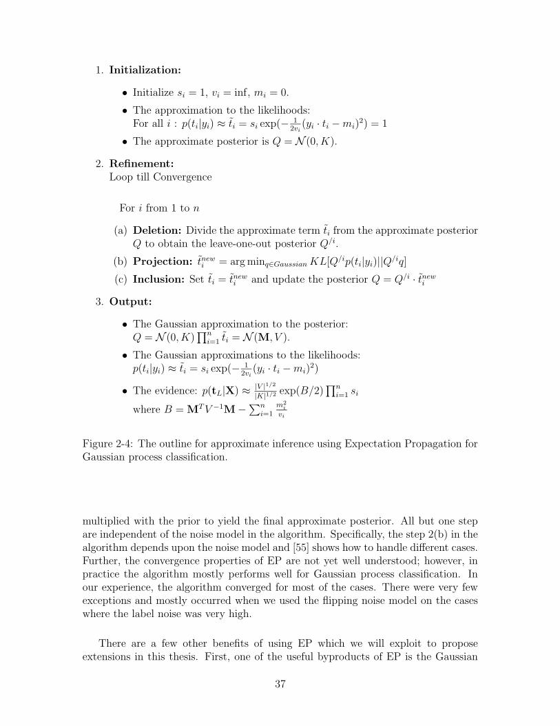
multiplied with the prior to yield the final approximate posterior. All but one stepare independent of the noise model in the algorithm. Specifically, the step 2(b) in thealgorithm depends upon the noise model and [55] shows how to handle different cases.Further, the convergence properties of EP are not yet well understood; however, inpractice the algorithm mostly performs well for Gaussian process classification. Inour experience, the algorithm converged for most of the cases. There were very fewexceptions and mostly occurred when we used the flipping noise model on the caseswhere the label noise was very high.

There are a few other benefits of using EP which we will exploit to proposeextensions in this thesis. First, one of the useful byproducts of EP is the Gaussian

37

approximations of the likelihoods p(ti|yi):

p(ti|yi) ≈ ti = si exp(−1

2vi

(yi · ti −mi)2) (2.6)

Note, that if we wish to exclude (include) a data point from the training set all weneed to do is divide (multiply) the posterior by the Gaussian approximation termcorresponding to the sample, which can be done efficiently. We will exploit this trickto train a mixture of Gaussian processes in chapter 3. Second, EP automaticallyprovides the normalization constant p(tL|X) for the posterior. This constant is calledthe evidence or the marginalized likelihood and can be used to learn hyperparametersof the model. We will use evidence maximization for hyperparameter and kernellearning in chapter 4 for semi-supervised scenarios.

2.2.2 Representing the Posterior Mean and the Covariance

As mentioned earlier, the full Bayesian treatment requires computing the integralgiven in equation 2.1 and it might seem that we need to perform Bayesian inferenceevery time we need to classify a test point. However, there is a nice representation ofthe posterior mean as well as the covariance in terms of the kernel, which allows usto express the Bayes point as a kernel classifier. Details of the proof can be found in[17].

Specifically, given a prior distribution p(y|X) ∼ N (0, K), for any data point xthe corresponding mean and the covariance of the posterior p(y|D), can be writtenas:

E[yx] = yx =n

∑

i=1

αi · k(xi,x) where, αi ∈ IR

E[(yx − yx)(yx′ − yx′ )] = k(x,x′

) +n

∑

i,j=1

k(x,xi) · βij · k(xj,x′

) where, βij ∈ IR

We can either use the the mean as a point classifier or use equation 2.1 to classifyany test points easily by using the representations mentioned above.

2.3 Hyperparameter Learning

The performance of the Gaussian process classification depends upon the kernel. Thenotion of similarity is captured using a kernel matrix and the performance is highlydependent upon the hyperparameters that describe the kernel. Further, there areparameters in the noise model (for example the slack penalty) and finding the rightset of all these parameters can be a challenge. Many discriminative models, includingSVMs often use cross-validation, which is a robust measure but can be prohibitively

38

expensive for real-world problems and problematic when we have few labeled datapoints.

Ideally we should be able to marginalize over these hyperparameters and therehave been approaches based on Hybrid Monte Carlo [87]. However, these approachesare expensive and empirical Bayes provides a computationally cheaper alternative.The idea here is to maximize the marginal likelihood or the evidence, which is noth-ing but the constant p(tL|X) that normalizes the posterior. This methodology oftuning the hyperparameter is often called evidence maximization and has been oneof the favorite tools for performing model selection. Evidence is a numerical quantityand signifies how well a model fits the given data. By comparing the evidence corre-sponding to the different models (or hyperparameters that determine the model), wecan choose the model and the hyperparameters suitable for the task.

Let us denote the hyperparameters of the model as Θ, which contains all thehyperparameters of the kernel as well as the parameter of the noise model. Formally,the idea behind evidence maximization is to choose a set of hyperparameters thatmaximize the evidence. That is, Θ = arg maxΘ log[p(tL|X,Θ)].

Note that we get evidence as a byproduct when using EP (see figure 2-4). Whenthe parameter space is small then a simple line search or the Matlab function fminbnd,based on golden section search and parabolic interpolation, can be used. However,in the case of a large parameter space exhaustive search is not feasible. In thosecases, non-linear optimization techniques, such as gradient descent or ExpectationMaximization (EM) can be used to optimize the evidence. However, the gradients ofevidence are not easy to compute despite the fact that the evidence is a byproductof EP.

In the past, there have been a few approaches that learn hyperparameters usingevidence maximization. Notable among them are [18, 23], which are based on vari-ational lower bounds and saddle point approximations. The EM-EP algorithm [39]is an alternative suitable when EP is used for approximate inference. The algorithmmaximizes evidence based on the variational lower bound and similar ideas have beenalso outlined by Seeger [75]. In the E-step of the algorithm EP is used to infer theposterior q(y) over the soft labels. The M-step consists of maximizing the variationallower bound:

F =

∫

y

q(y) logp(y|X, Θ)p(tL|y, Θ)

q(y)

= −

∫

y

q(y) log q(y) +

∫

y

q(y) logN (y; 0, K)

+n

∑

i=1

∫

yi

q(yi) log p(ti|yi) ≤ p(tL|X, Θ)

The EM procedure alternates between the E-step and the M-step until convergence.

• E-Step: Given the current parameters Θi, approximate the posterior q(y) ∼N (y,Σy) by EP.

• M-Step: Update Θi+1 = arg maxΘ

∫

yq(y) log p(y|X,Θ)p(tL|y,Θ)

q(y)

39

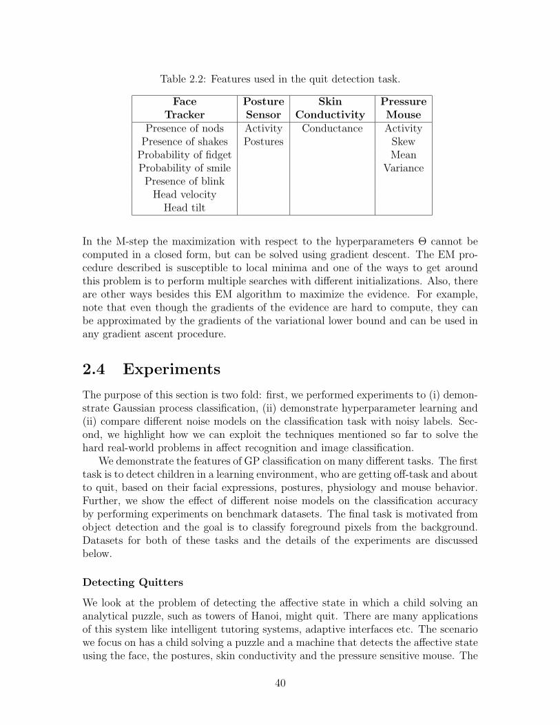
Table 2.2: Features used in the quit detection task.

Face Posture Skin PressureTracker Sensor Conductivity Mouse

Presence of nods Activity Conductance ActivityPresence of shakes Postures Skew

Probability of fidget MeanProbability of smile VariancePresence of blink

Head velocityHead tilt

In the M-step the maximization with respect to the hyperparameters Θ cannot becomputed in a closed form, but can be solved using gradient descent. The EM pro-cedure described is susceptible to local minima and one of the ways to get aroundthis problem is to perform multiple searches with different initializations. Also, thereare other ways besides this EM algorithm to maximize the evidence. For example,note that even though the gradients of the evidence are hard to compute, they canbe approximated by the gradients of the variational lower bound and can be used inany gradient ascent procedure.

2.4 Experiments

The purpose of this section is two fold: first, we performed experiments to (i) demon-strate Gaussian process classification, (ii) demonstrate hyperparameter learning and(ii) compare different noise models on the classification task with noisy labels. Sec-ond, we highlight how we can exploit the techniques mentioned so far to solve thehard real-world problems in affect recognition and image classification.

We demonstrate the features of GP classification on many different tasks. The firsttask is to detect children in a learning environment, who are getting off-task and aboutto quit, based on their facial expressions, postures, physiology and mouse behavior.Further, we show the effect of different noise models on the classification accuracyby performing experiments on benchmark datasets. The final task is motivated fromobject detection and the goal is to classify foreground pixels from the background.Datasets for both of these tasks and the details of the experiments are discussedbelow.

Detecting Quitters

We look at the problem of detecting the affective state in which a child solving ananalytical puzzle, such as towers of Hanoi, might quit. There are many applicationsof this system like intelligent tutoring systems, adaptive interfaces etc. The scenariowe focus on has a child solving a puzzle and a machine that detects the affective stateusing the face, the postures, skin conductivity and the pressure sensitive mouse. The

40

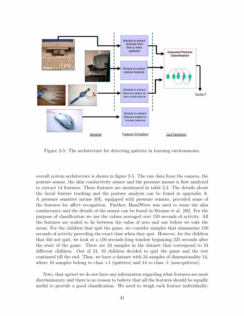
Figure 2-5: The architecture for detecting quitters in learning environments.

overall system architecture is shown in figure 2-5. The raw data from the camera, theposture sensor, the skin conductivity sensor and the pressure mouse is first analyzedto extract 14 features. These features are mentioned in table 2.2. The details aboutthe facial feature tracking and the posture analysis can be found in appendix A.A pressure sensitive mouse [69], equipped with pressure sensors, provided some ofthe features for affect recognition. Further, HandWave was used to sense the skinconductance and the details of the sensor can be found in Strauss et al. [80]. For thepurpose of classification we use the values averaged over 150 seconds of activity. Allthe features are scaled to lie between the value of zero and one before we take themean. For the children that quit the game, we consider samples that summarize 150seconds of activity preceding the exact time when they quit. However, for the childrenthat did not quit, we look at a 150 seconds long window beginning 225 seconds afterthe start of the game. There are 24 samples in the dataset that correspond to 24different children. Out of 24, 10 children decided to quit the game and the restcontinued till the end. Thus, we have a dataset with 24 samples of dimensionality 14,where 10 samples belong to class +1 (quitters) and 14 to class -1 (non-quitters).

Note, that apriori we do not have any information regarding what features are mostdiscriminatory and there is no reason to believe that all the features should be equallyuseful to provide a good classification. We need to weigh each feature individually;

41

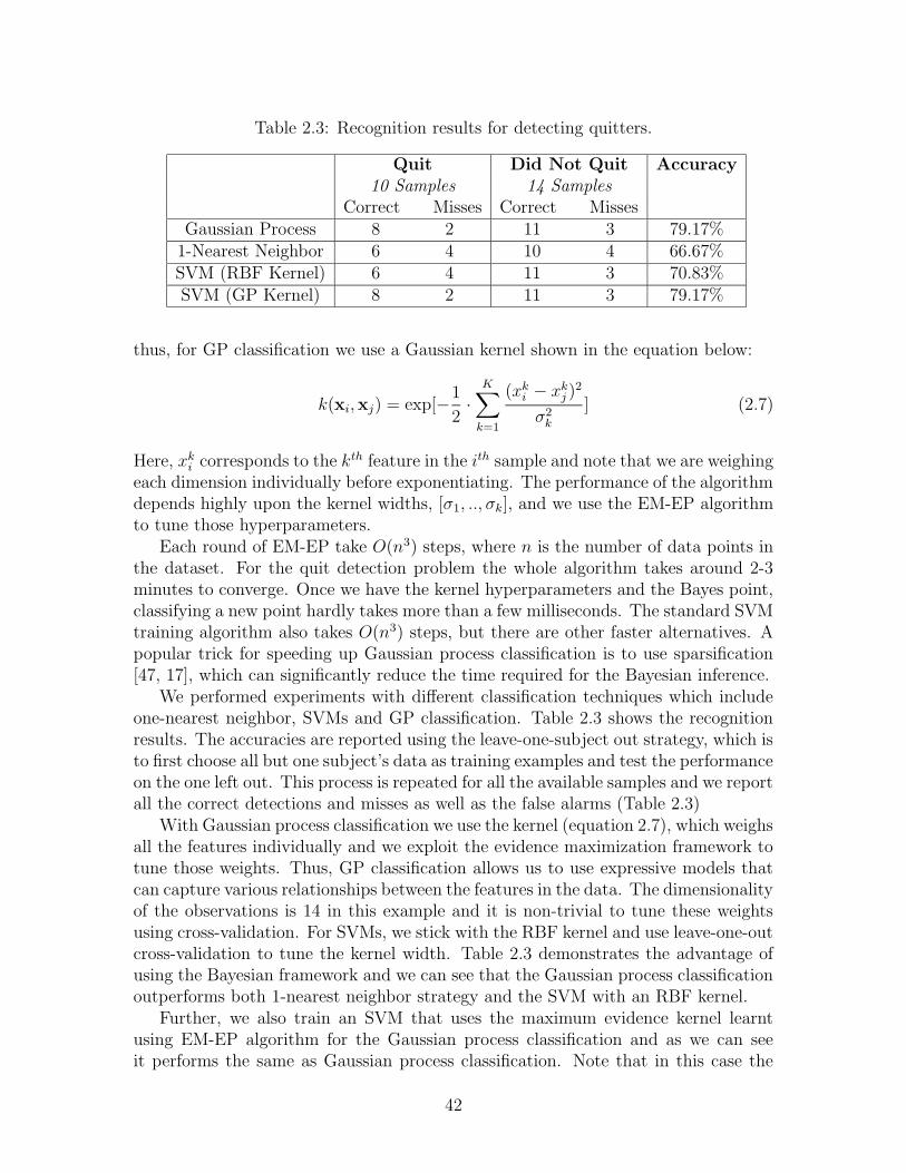
Table 2.3: Recognition results for detecting quitters.

Quit Did Not Quit Accuracy10 Samples 14 Samples

Correct Misses Correct MissesGaussian Process 8 2 11 3 79.17%

1-Nearest Neighbor 6 4 10 4 66.67%SVM (RBF Kernel) 6 4 11 3 70.83%SVM (GP Kernel) 8 2 11 3 79.17%

thus, for GP classification we use a Gaussian kernel shown in the equation below:

k(xi,xj) = exp[−1

2·

K∑

k=1

(xki − xk

j )2

σ2k

] (2.7)

Here, xki corresponds to the kth feature in the ith sample and note that we are weighing

each dimension individually before exponentiating. The performance of the algorithmdepends highly upon the kernel widths, [σ1, .., σk], and we use the EM-EP algorithmto tune those hyperparameters.

Each round of EM-EP take O(n3) steps, where n is the number of data points inthe dataset. For the quit detection problem the whole algorithm takes around 2-3minutes to converge. Once we have the kernel hyperparameters and the Bayes point,classifying a new point hardly takes more than a few milliseconds. The standard SVMtraining algorithm also takes O(n3) steps, but there are other faster alternatives. Apopular trick for speeding up Gaussian process classification is to use sparsification[47, 17], which can significantly reduce the time required for the Bayesian inference.

We performed experiments with different classification techniques which includeone-nearest neighbor, SVMs and GP classification. Table 2.3 shows the recognitionresults. The accuracies are reported using the leave-one-subject out strategy, which isto first choose all but one subject’s data as training examples and test the performanceon the one left out. This process is repeated for all the available samples and we reportall the correct detections and misses as well as the false alarms (Table 2.3)

With Gaussian process classification we use the kernel (equation 2.7), which weighsall the features individually and we exploit the evidence maximization framework totune those weights. Thus, GP classification allows us to use expressive models thatcan capture various relationships between the features in the data. The dimensionalityof the observations is 14 in this example and it is non-trivial to tune these weightsusing cross-validation. For SVMs, we stick with the RBF kernel and use leave-one-outcross-validation to tune the kernel width. Table 2.3 demonstrates the advantage ofusing the Bayesian framework and we can see that the Gaussian process classificationoutperforms both 1-nearest neighbor strategy and the SVM with an RBF kernel.

Further, we also train an SVM that uses the maximum evidence kernel learntusing EM-EP algorithm for the Gaussian process classification and as we can seeit performs the same as Gaussian process classification. Note that in this case the

42

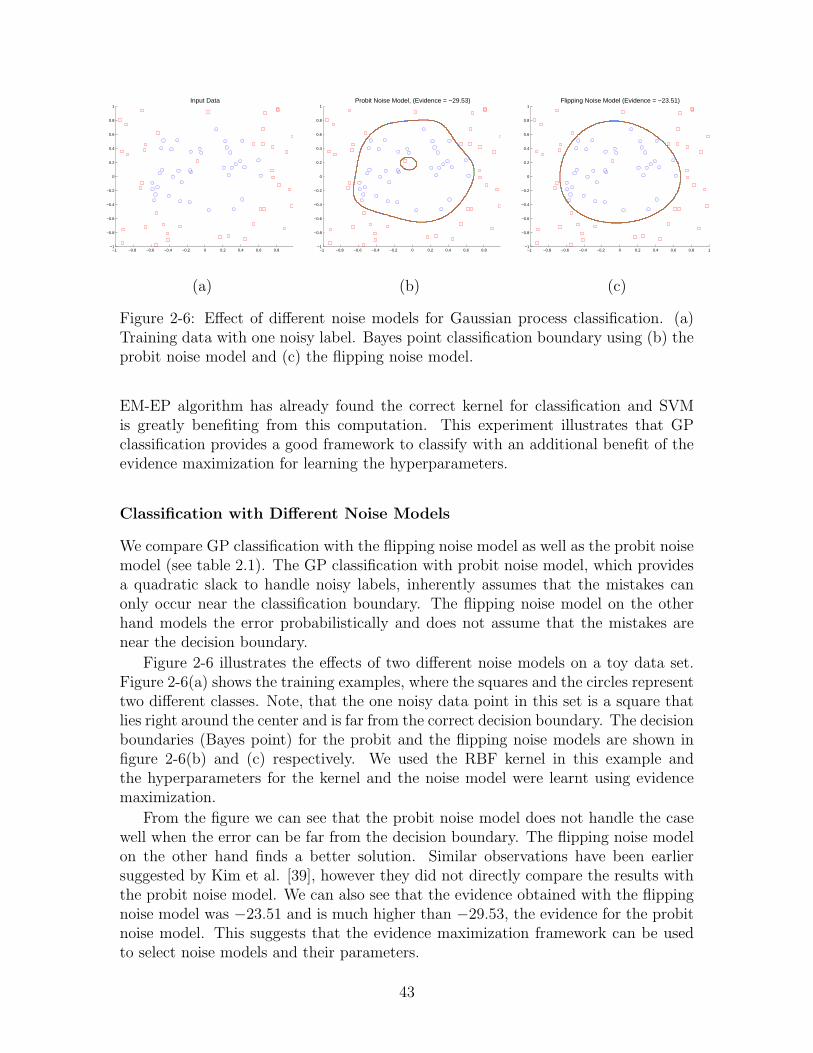
−1 −0.8 −0.6 −0.4 −0.2 0 0.2 0.4 0.6 0.8 1−1

−0.8

−0.6

−0.4

−0.2

0

0.2

0.4

0.6

0.8

1Input Data

−1 −0.8 −0.6 −0.4 −0.2 0 0.2 0.4 0.6 0.8 1−1

−0.8

−0.6

−0.4

−0.2

0

0.2

0.4

0.6

0.8

1Probit Noise Model, (Evidence = −29.53)

−1 −0.8 −0.6 −0.4 −0.2 0 0.2 0.4 0.6 0.8 1−1

−0.8

−0.6

−0.4

−0.2

0

0.2

0.4

0.6

0.8

1Flipping Noise Model (Evidence = −23.51)

(a) (b) (c)

Figure 2-6: Effect of different noise models for Gaussian process classification. (a)Training data with one noisy label. Bayes point classification boundary using (b) theprobit noise model and (c) the flipping noise model.

EM-EP algorithm has already found the correct kernel for classification and SVMis greatly benefiting from this computation. This experiment illustrates that GPclassification provides a good framework to classify with an additional benefit of theevidence maximization for learning the hyperparameters.

Classification with Different Noise Models

We compare GP classification with the flipping noise model as well as the probit noisemodel (see table 2.1). The GP classification with probit noise model, which providesa quadratic slack to handle noisy labels, inherently assumes that the mistakes canonly occur near the classification boundary. The flipping noise model on the otherhand models the error probabilistically and does not assume that the mistakes arenear the decision boundary.

Figure 2-6 illustrates the effects of two different noise models on a toy data set.Figure 2-6(a) shows the training examples, where the squares and the circles representtwo different classes. Note, that the one noisy data point in this set is a square thatlies right around the center and is far from the correct decision boundary. The decisionboundaries (Bayes point) for the probit and the flipping noise models are shown infigure 2-6(b) and (c) respectively. We used the RBF kernel in this example andthe hyperparameters for the kernel and the noise model were learnt using evidencemaximization.

From the figure we can see that the probit noise model does not handle the casewell when the error can be far from the decision boundary. The flipping noise modelon the other hand finds a better solution. Similar observations have been earliersuggested by Kim et al. [39], however they did not directly compare the results withthe probit noise model. We can also see that the evidence obtained with the flippingnoise model was −23.51 and is much higher than −29.53, the evidence for the probitnoise model. This suggests that the evidence maximization framework can be usedto select noise models and their parameters.

43

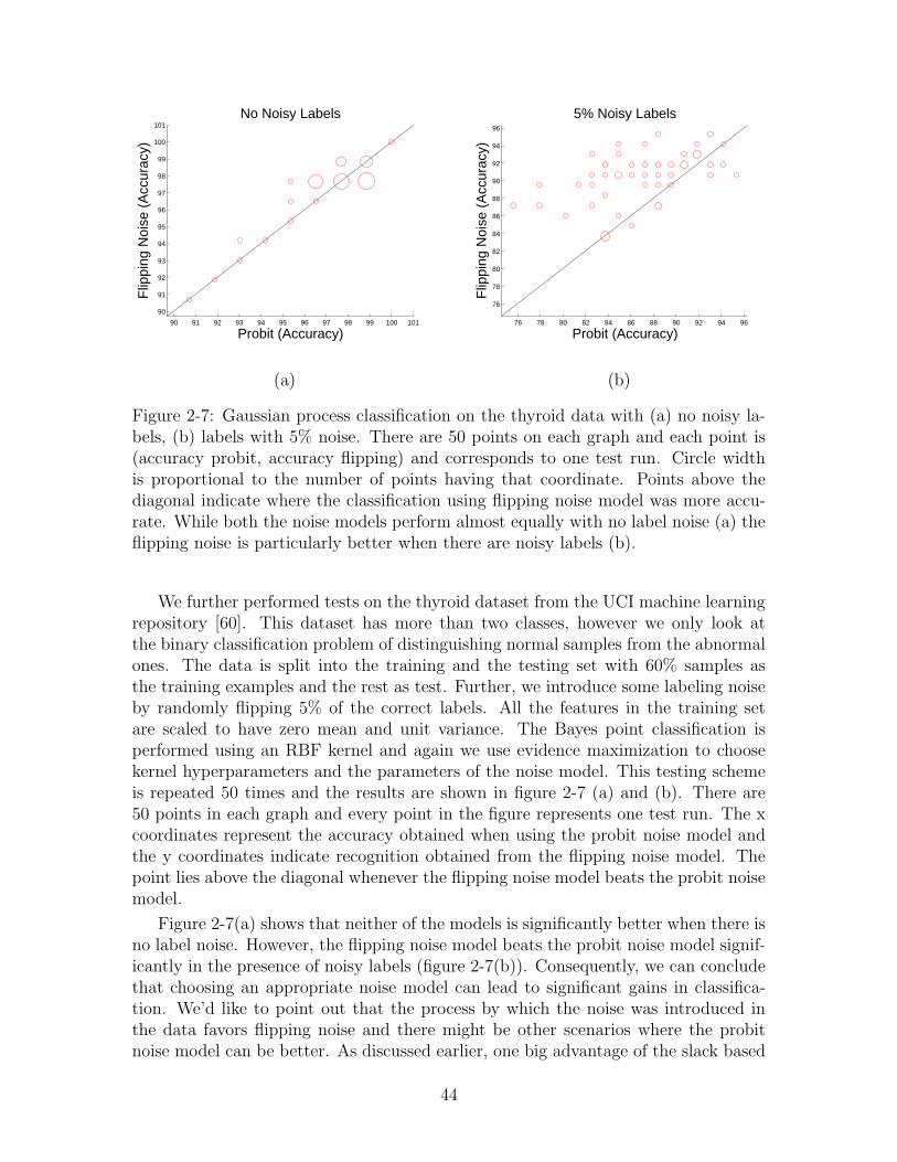
90 91 92 93 94 95 96 97 98 99 100 101

90

91

92

93

94

95

96

97

98

99

100

101

Flip

ping

Noi

se (

Acc

urac

y)

Probit (Accuracy)

No Noisy Labels

76 78 80 82 84 86 88 90 92 94 96

76

78

80

82

84

86

88

90

92

94

96

Flip

ping

Noi

se (

Acc

urac

y)

Probit (Accuracy)

5% Noisy Labels

(a) (b)

Figure 2-7: Gaussian process classification on the thyroid data with (a) no noisy la-bels, (b) labels with 5% noise. There are 50 points on each graph and each point is(accuracy probit, accuracy flipping) and corresponds to one test run. Circle widthis proportional to the number of points having that coordinate. Points above thediagonal indicate where the classification using flipping noise model was more accu-rate. While both the noise models perform almost equally with no label noise (a) theflipping noise is particularly better when there are noisy labels (b).

We further performed tests on the thyroid dataset from the UCI machine learningrepository [60]. This dataset has more than two classes, however we only look atthe binary classification problem of distinguishing normal samples from the abnormalones. The data is split into the training and the testing set with 60% samples asthe training examples and the rest as test. Further, we introduce some labeling noiseby randomly flipping 5% of the correct labels. All the features in the training setare scaled to have zero mean and unit variance. The Bayes point classification isperformed using an RBF kernel and again we use evidence maximization to choosekernel hyperparameters and the parameters of the noise model. This testing schemeis repeated 50 times and the results are shown in figure 2-7 (a) and (b). There are50 points in each graph and every point in the figure represents one test run. The xcoordinates represent the accuracy obtained when using the probit noise model andthe y coordinates indicate recognition obtained from the flipping noise model. Thepoint lies above the diagonal whenever the flipping noise model beats the probit noisemodel.

Figure 2-7(a) shows that neither of the models is significantly better when there isno label noise. However, the flipping noise model beats the probit noise model signif-icantly in the presence of noisy labels (figure 2-7(b)). Consequently, we can concludethat choosing an appropriate noise model can lead to significant gains in classifica-tion. We’d like to point out that the process by which the noise was introduced inthe data favors flipping noise and there might be other scenarios where the probitnoise model can be better. As discussed earlier, one big advantage of the slack based

44

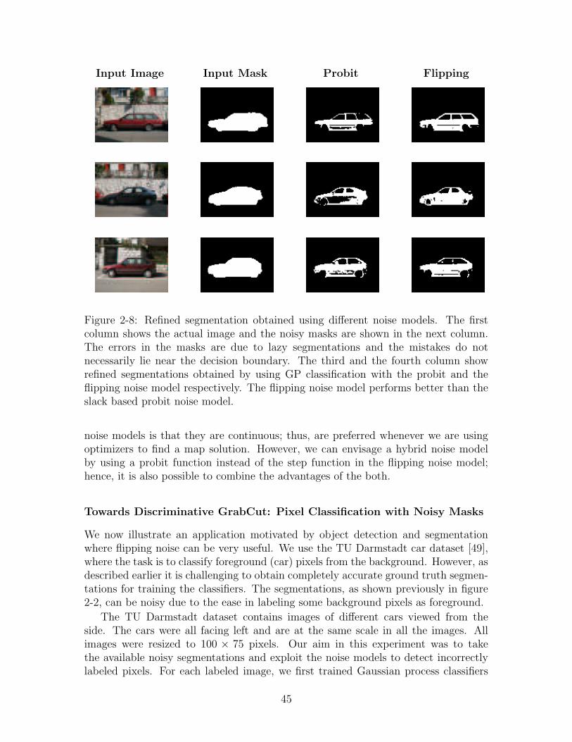
Input Image Input Mask Probit Flipping

Figure 2-8: Refined segmentation obtained using different noise models. The firstcolumn shows the actual image and the noisy masks are shown in the next column.The errors in the masks are due to lazy segmentations and the mistakes do notnecessarily lie near the decision boundary. The third and the fourth column showrefined segmentations obtained by using GP classification with the probit and theflipping noise model respectively. The flipping noise model performs better than theslack based probit noise model.

noise models is that they are continuous; thus, are preferred whenever we are usingoptimizers to find a map solution. However, we can envisage a hybrid noise modelby using a probit function instead of the step function in the flipping noise model;hence, it is also possible to combine the advantages of the both.

Towards Discriminative GrabCut: Pixel Classification with Noisy Masks

We now illustrate an application motivated by object detection and segmentationwhere flipping noise can be very useful. We use the TU Darmstadt car dataset [49],where the task is to classify foreground (car) pixels from the background. However, asdescribed earlier it is challenging to obtain completely accurate ground truth segmen-tations for training the classifiers. The segmentations, as shown previously in figure2-2, can be noisy due to the ease in labeling some background pixels as foreground.

The TU Darmstadt dataset contains images of different cars viewed from theside. The cars were all facing left and are at the same scale in all the images. Allimages were resized to 100 × 75 pixels. Our aim in this experiment was to takethe available noisy segmentations and exploit the noise models to detect incorrectlylabeled pixels. For each labeled image, we first trained Gaussian process classifiers

45

with the different noise models using the available segmentations. The pixel featuresused in classification were the rgb values. We use a linear kernel for all of thesemethods and the only difference is the noise model. Once trained, we apply theclassifier to the training image itself to obtain a refined labeling. This procedure canbe iterated to obtain better segmentations. Note, that this scheme can be thoughtof as a discriminative version of grabcut [70]. Grabcut is an object segmentationscheme that aims to classify the foreground pixels from the background given animage annotated for a region that contains most of the foreground. The grabcutuses generative models together with spatial smoothness constraints to provide therequired segmentation. Note, that the scheme described in this section is a simplerversion as there are no spatial constraints that impose spatial smoothness; however,these constraints can be easily introduced using a Conditional Random Field (CRF)formulation (see Chapter 5).

Figure 2-8 shows segmentation results using the GP classification with differentnoise models. GP classification with the flipping noise model provides the mostconvincing segmentation as the labels provided for training are noisy due to lazysegmentation of the training images. The GP classification with the probit modelthat provides quadratic slack do not do that well as it assumes that the mistakesare near the decision boundary. There are other salt and pepper noise in the finalsegmentations, which we remove by multiplying the classification result with theoriginal training mask. We can also tackle this problem using spatial smoothing andimposing long range dependencies. Further, our choice of features is pretty simple inthis experiment. In chapter 5 we will see how to address many of these issues.

2.5 Conclusions and Extensions

In this chapter we introduced Gaussian process classification with different noisemodels, together with the basic ideas behind the approximate Bayesian inferenceand hyperparameter learning. We demonstrated hyperparameter learning and clas-sification on an affect recognition task, where the goal was to detect quitters usingobservations recorded from face, posture, pressure and skin conductivity. Further, wedemonstrated using synthetic examples, benchmark datasets and a pixel classificationtask that choosing a good noise model can improve recognition performance.

Gaussian Process Classification with Incomplete Data

Gaussian process classification aims to directly model the decision boundary giventhe training data and it is not trivial to handle all cases of incompleteness in the datawith these models. Out of the four cases of incompleteness handled in this thesis, theclassic GP classification has capabilities to handle only one of them. As discussed insection 2.1.2, we have shown how to use different noise models to handle the case ofincorrect labels. We briefly describe difficulties associated with the rest of the casesas a roadmap for the rest of this thesis:

46

• Incomplete Features: One never models the underlying data density p(x) inGP classification; thus, handling the case of missing features in the observationsis not straight forward. The smoothness constraint in GP classification dependsupon the kernel matrix K, which is hard to compute with incomplete features.In Chapter 3 we will provide extensions to GP classification using a mixture ofGaussian processes.

• Partially Labeled Data: As shown in this chapter, GP classifiers first assumea smoothness constraint (the GP prior) and then incorporate information fromthe labeled data only. The smoothness constraint only encodes the assumptionthat similar data points should have the same label and is independent of theunderlying data density. Hence, any information from the unlabeled data isunused. In Chapter 4, we will show how to use data dependent regularizationto tackle this case of incompleteness.

• Coarse Labels: Gaussian process classification provides a nice framework forprobabilistic discrimination of the data but in the original form is just limitedto the supervised classification scenarios. In Chapter 5 we will show how we canexploit the flexibility provided by the Bayesian discriminative models to encodeprior knowledge about the problem using various graphical models.

47

48

Chapter 3

Mixture of Gaussian Processes forCombining Multiple Modalities

This chapter1 describes a unified approach based on Gaussian Processes for achievingsensor fusion under the problematic conditions of missing channels and noisy labels.There are a growing number of scenarios in pattern recognition where multimodalinformation is used, and where information from multiple sensors needs to be fusedto recover the variable of interest. Multi-sensor classification is a problem that hasbeen addressed previously by using either data-level fusion or classifier combinationschemes. In the former, a single classifier is trained on joint features; however, whenthe data has even one missing channel, a frequent problem, then usually all the datais ignored for that time block, resulting in a significant reduction in the total amountof data for training.

We propose to handle the incompleteness resulting from missing features usinga mixture of Gaussian Processes. Note that marginalization of incomplete featuresrequires explicit modeling of the probability density over the observations, whichcan be hard to model correctly when the dimensionality of the observations is bigcompared to the number of training examples. Rather than marginalizing over themissing data, the basic idea behind the proposed framework is to combine decisionsof individual classifiers trained on different subsets of the features. Consequently,whenever there are missing features the decision level fusion ignores the contributionfrom the classifiers that act on the set of missing features. There are a lot of waysto combine the decisions, and the proposed framework exploits the idea behind themixture-of-experts [30] and, as shown in the experiments section, is a better choicethan most of the rule-based methods. Under the proposed approach, Gaussian Pro-cesses generate separate class labels corresponding to each individual modality. Thefinal classification is based upon a hidden random variable, which probabilisticallycombines the sensors. Given both labeled and test data, the inference on unknownvariables, parameters and class labels for the test data is performed using the varia-tional bound and Expectation Propagation. There are big computational advantages

1The work described in this chapter appeared in the ACM Conference on Multimedia, 2005 [35]and the Workshop on Multiple Classifier Systems, 2005 [32]

49

of using this framework as for each expert the posterior over the class labels is obtainedvia Expectation Propagation. Hence, the approximate posterior over each classifica-tion function is a product of Gaussians and can be updated very quickly, resulting inhuge computational savings.

The proposed extension can be combined easily with other extensions proposedin this thesis. For example, this model can be extended to handle the case of noisylabels and can be applied to the highly challenging problems combining many ofthe incompleteness scenarios described in the first chapter, such as semi-supervisedcases with multi-sensory data, where channels are frequently missing and there mightbe labeling errors in the data. We apply this method to the challenge of detectingthe affective state of interest in children trying to solve a puzzle, combining sensoryinformation from the face, the postures and the state of the puzzle task, to infer thestudent’s state. Classification with the proposed new approach achieves accuracy ofover 86%, significantly outperforming the classification using individual modalitiesand other common classifier combination schemes.

3.1 Previous Work

Classification with Incomplete Data: Classifiers based on the generative paradigmexplicitly model the underlying distribution of the observations and can be used eas-ily with missing data by integrating out the incomplete features. The discriminativemodels on the other hand never explicitly model the observation density; thus, theycannot easily handle the incompleteness in features. One of the popular methods toget around this problem is to use imputation, where the missing data is filled withspecific values, such as zeros or the mean of the distribution. There are other al-ternatives that require explicit models of the probability density of the observations.For example, Williams et al. [89] use a mixture of Gaussians to model the densityof observations. Then, there are methods described in Rubin [71] based on samplingfrom the underlying observation density. As these methods explicitly model the datadistribution, they can encounter problems when the dimensionality of the observationis huge as compared to the number of available training examples. Also, there aremethods based on kernel completion [24, 85], where the idea is to complete the kernelmatrix based on some optimization criteria or other auxiliary observations. However,these methods do not take into account the uncertainty of the missing features andit is not clear how well they perform when the kernel matrices are sparse.

The work presented in this chapter proposes an alternative way to handle the in-completeness. The idea is to train classifiers based on different subsets of features andthen use a classifier combination strategy to provide a final decision. Whenever theframework encounters missing features in the data, the decision level fusion ignoresthose classifiers that act on missing data. Note that this framework does not everexplicitly model the underlying observation density; thus, it can be used in scenar-ios where the dimensionality of the observations is big compared to the number ofexamples.

Classifier Combination: A lot of researchers have looked into the general problem

50

of combining information from multiple channels. There are many methods, includingBoosting [73] and Bagging [9], which generate an ensemble of classifiers by choosingdifferent samples from the training set. These methods require a common set oftraining data, which is a set of joint vectors formed by stacking the features extractedfrom all the modalities into one big vector. As mentioned earlier, often in multi-sensorfusion problems the sensors or feature extraction might fail, resulting in data withmissing channels; thus, most of the data cannot be used to form a common set oftraining data. Similarly, most of the data remains unused in “feature-level fusion,”where a single classifier is trained on joint features.

One alternate solution is to use decision-level fusion. Kittler et al. [40] have de-scribed a common framework for combining classifiers and provided theoretical justifi-cation for using simple operators such as majority vote, sum, product, maximum andminimum. Hong and Jain [27] have used a similar framework to fuse multiple modali-ties for personal identification. Similarly, Han and Bhanu [25] also perform rule-basedfusion for gait-based human recognition. One problem with these fixed rules is that,it is difficult to predict which rule would perform best. Then there are methods,such as layered HMMs proposed by Oliver et al. [62], which perform decision fusionand sensor selection depending upon utility functions and stacked classifiers. Onemain disadvantage of using stacked based classification is that these methods requirea large amount of labeled training data. Alternatively, there are other mixture-of-experts [30] and critic-driven approaches [53, 29] where base-level classifiers (experts)are combined using second level classifiers (critics or gating functions) that predicthow well an expert is going to perform on the current input. To make a classifierselection, the critic can either look at the current input or base its decision upon someother contextual features as well. For example, Toyama and Horvitz [83] demonstratea head tracking system based on multiple algorithms, that uses contextual features asreliability indicators for the different tracking algorithms. In an earlier work [36] wehave proposed an expert-critic system based on HMMs to combine multiple modal-ities. In this work we showed an alternative fusion strategy within the Bayesianframework which significantly beats the earlier method. The framework describedhere is also based on sensor-selection and is most similar to Tresp [84], where themixture of Gaussian Processes is described. The key differences include classificationbased on Gaussian Process rather than regression; also, we use Expectation Propa-gation for Gaussian Process classification and our classification likelihood is robustto labeling errors and noise. Our framework is also capable of quickly re-learningthe classification given updated label associations. Further, we provide a completeBayesian treatment of the problem rather than using a maximum-likelihood training.Affect Recognition: A lot of research has been done to develop methods for infer-ring affective states. Many researchers have used static methods such as question-naires, dialogue boxes, etc., which are easy to administer but have been criticizedfor being static and thus not able to recognize changes in affective states. A moredynamic and objective approach for sensing affect is via sensors such as cameras,microphones, wearable devices, etc. However, most of the work on affect recognitionusing the sensors focuses on deliberately expressed emotions (happy /sad /angry etc.)by actors, and not on those that arise in natural situations such as classroom learn-

51

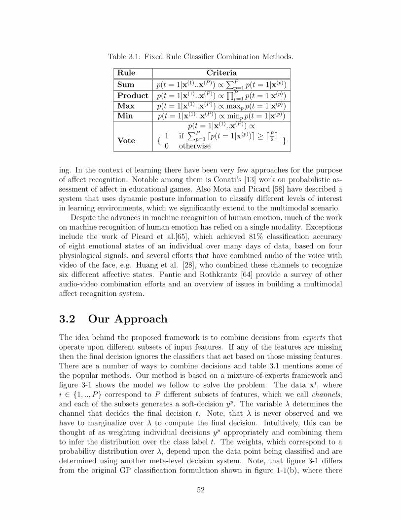
Table 3.1: Fixed Rule Classifier Combination Methods.

Rule Criteria

Sum p(t = 1|x(1)..x(P )) ∝∑P

p=1 p(t = 1|x(p))

Product p(t = 1|x(1)..x(P )) ∝∏P

p=1 p(t = 1|x(p))

Max p(t = 1|x(1)..x(P )) ∝ maxp p(t = 1|x(p))

Min p(t = 1|x(1)..x(P )) ∝ minp p(t = 1|x(p))

p(t = 1|x(1)..x(P )) ∝

Vote {1 if

∑Pp=1 dp(t = 1|x(p))e ≥ dP

2e

0 otherwise}

ing. In the context of learning there have been very few approaches for the purposeof affect recognition. Notable among them is Conati’s [13] work on probabilistic as-sessment of affect in educational games. Also Mota and Picard [58] have described asystem that uses dynamic posture information to classify different levels of interestin learning environments, which we significantly extend to the multimodal scenario.

Despite the advances in machine recognition of human emotion, much of the workon machine recognition of human emotion has relied on a single modality. Exceptionsinclude the work of Picard et al.[65], which achieved 81% classification accuracyof eight emotional states of an individual over many days of data, based on fourphysiological signals, and several efforts that have combined audio of the voice withvideo of the face, e.g. Huang et al. [28], who combined these channels to recognizesix different affective states. Pantic and Rothkrantz [64] provide a survey of otheraudio-video combination efforts and an overview of issues in building a multimodalaffect recognition system.

3.2 Our Approach

The idea behind the proposed framework is to combine decisions from experts thatoperate upon different subsets of input features. If any of the features are missingthen the final decision ignores the classifiers that act based on those missing features.There are a number of ways to combine decisions and table 3.1 mentions some ofthe popular methods. Our method is based on a mixture-of-experts framework andfigure 3-1 shows the model we follow to solve the problem. The data xi, wherei ∈ {1, .., P} correspond to P different subsets of features, which we call channels,and each of the subsets generates a soft-decision yp. The variable λ determines thechannel that decides the final decision t. Note, that λ is never observed and wehave to marginalize over λ to compute the final decision. Intuitively, this can bethought of as weighting individual decisions yp appropriately and combining themto infer the distribution over the class label t. The weights, which correspond to aprobability distribution over λ, depend upon the data point being classified and aredetermined using another meta-level decision system. Note, that figure 3-1 differsfrom the original GP classification formulation shown in figure 1-1(b), where there

52

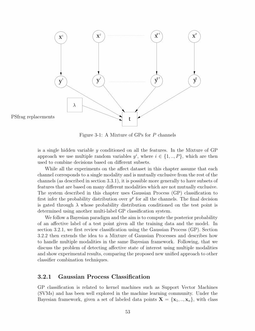
21x x x x

t

1 2

y y y

p-1 p

p-1 yp

PSfrag replacements

λ

Figure 3-1: A Mixture of GPs for P channels

is a single hidden variable y conditioned on all the features. In the Mixture of GPapproach we use multiple random variables yi, where i ∈ {1, .., P}, which are thenused to combine decisions based on different subsets.

While all the experiments on the affect dataset in this chapter assume that eachchannel corresponds to a single modality and is mutually exclusive from the rest of thechannels (as described in section 3.3.1), it is possible more generally to have subsets offeatures that are based on many different modalities which are not mutually exclusive.The system described in this chapter uses Gaussian Process (GP) classification tofirst infer the probability distribution over yp for all the channels. The final decisionis gated through λ whose probability distribution conditioned on the test point isdetermined using another multi-label GP classification system.

We follow a Bayesian paradigm and the aim is to compute the posterior probabilityof an affective label of a test point given all the training data and the model. Insection 3.2.1, we first review classification using the Gaussian Process (GP). Section3.2.2 then extends the idea to a Mixture of Gaussian Processes and describes howto handle multiple modalities in the same Bayesian framework. Following, that wediscuss the problem of detecting affective state of interest using multiple modalitiesand show experimental results, comparing the proposed new unified approach to otherclassifier combination techniques.

3.2.1 Gaussian Process Classification

GP classification is related to kernel machines such as Support Vector Machines(SVMs) and has been well explored in the machine learning community. Under theBayesian framework, given a set of labeled data points X = {x1, ..,xn}, with class

53

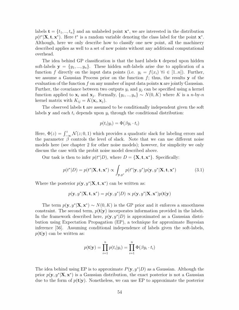
labels t = {t1, .., tn} and an unlabeled point x∗, we are interested in the distributionp(t∗|X, t,x∗). Here t∗ is a random variable denoting the class label for the point x∗.Although, here we only describe how to classify one new point, all the machinerydescribed applies as well to a set of new points without any additional computationaloverhead.

The idea behind GP classification is that the hard labels t depend upon hiddensoft-labels y = {y1, ..., yn}. These hidden soft-labels arise due to application of afunction f directly on the input data points (i.e. yi = f(xi) ∀i ∈ [1..n]). Further,we assume a Gaussian Process prior on the function f ; thus, the results y of theevaluation of the function f on any number of input data points x are jointly Gaussian.Further, the covariance between two outputs yi and yj can be specified using a kernelfunction applied to xi and xj. Formally, {y1, .., yn} ∼ N(0, K) where K is a n-by-nkernel matrix with Kij = K(xi,xj).

The observed labels t are assumed to be conditionally independent given the softlabels y and each ti depends upon yi through the conditional distribution:

p(ti|yi) = Φ(βyi · ti)

Here, Φ(z) =∫ z

−∞N (z; 0, 1) which provides a quadratic slack for labeling errors and

the parameter β controls the level of slack. Note that we can use different noisemodels here (see chapter 2 for other noise models); however, for simplicity we onlydiscuss the case with the probit noise model described above.

Our task is then to infer p(t∗|D), where D = {X, t,x∗}. Specifically:

p(t∗|D) = p(t∗|X, t,x∗) ∝

∫

y,y∗

p(t∗|y, y∗)p(y, y∗|X, t,x∗) (3.1)

Where the posterior p(y, y∗|X, t,x∗) can be written as:

p(y, y∗|X, t,x∗) = p(y, y∗|D) ∝ p(y, y∗|X,x∗)p(t|y)

The term p(y, y∗|X,x∗) ∼ N(0, K) is the GP prior and it enforces a smoothnessconstraint. The second term, p(t|y) incorporates information provided in the labels.In the framework described here, p(y, y∗|D) is approximated as a Gaussian distri-bution using Expectation Propagation (EP), a technique for approximate Bayesianinference [56]. Assuming conditional independence of labels given the soft-labels,p(t|y) can be written as:

p(t|y) =n

∏

i=1

p(ti|yi) =n

∏

i=1

Φ(βyi · ti)

The idea behind using EP is to approximate P (y, y∗|D) as a Gaussian. Although theprior p(y, y∗|X,x∗) is a Gaussian distribution, the exact posterior is not a Gaussiandue to the form of p(t|y). Nonetheless, we can use EP to approximate the posterior

54

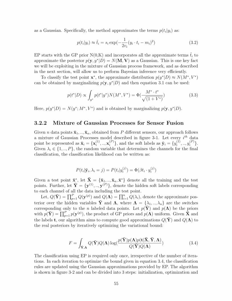
as a Gaussian. Specifically, the method approximates the terms p(ti|yi) as:

p(ti|yi) ≈ ti = si exp(−1

2vi

(yi · ti −mi)2) (3.2)

EP starts with the GP prior N(0,K) and incorporates all the approximate terms ti toapproximate the posterior p(y, y∗|D) = N(M,V) as a Gaussian. This is one key factwe will be exploiting in the mixture of Gaussian process framework, and as describedin the next section, will allow us to perform Bayesian inference very efficiently.

To classify the test point x∗, the approximate distribution p(y∗|D) ≈ N(M ∗, V ∗)can be obtained by marginalizing p(y, y∗|D) and then equation 3.1 can be used:

p(t∗|D) ∝

∫

y∗

p(t∗|y∗)N(M ∗, V ∗) = Φ(M∗ · t∗

√

(1 + V ∗)) (3.3)

Here, p(y∗|D) = N(y∗;M∗, V ∗) and is obtained by marginalizing p(y, y∗|D).

3.2.2 Mixture of Gaussian Processes for Sensor Fusion

Given n data points x1, .., xn, obtained from P different sensors, our approach followsa mixture of Gaussian Processes model described in figure 3-1. Let every ith datapoint be represented as xi = {x(1)

i , ..,x(P )i }, and the soft labels as yi = {y(1)

i , .., y(P )i }.

Given λi ∈ {1, .., P}, the random variable that determines the channels for the finalclassification, the classification likelihood can be written as:

P (ti|yi, λi = j) = P (ti|y(j)i ) = Φ(βti · y

(j)i )

Given a test point x∗, let X = {x1, .., xn, x∗} denote all the training and the test

points. Further, let Y = {y(1), ..,y(P )}, denote the hidden soft labels correspondingto each channel of all the data including the test point.

Let, Q(Y) =∏P

p=1Q(y(p)) and Q(Λ) =∏n

i=1Q(λi), denote the approximate pos-

terior over the hidden variables Y and Λ, where Λ = {λ1, .., λn} are the switchescorresponding only to the n labeled data points. Let p(Y) and p(Λ) be the priorswith p(Y) =

∏Pp=1 p(y

(p)), the product of GP priors and p(Λ) uniform. Given X and

the labels t, our algorithm aims to compute good approximations Q(Y) and Q(Λ) tothe real posteriors by iteratively optimizing the variational bound:

F =

∫

Y,Λ

Q(Y)Q(Λ) log(p(Y)p(Λ)p(t|X, Y,Λ)

Q(Y)Q(Λ)) (3.4)

The classification using EP is required only once, irrespective of the number of itera-tions. In each iteration to optimize the bound given in equation 3.4, the classificationrules are updated using the Gaussian approximations provided by EP. The algorithmis shown in figure 3-2 and can be divided into 3 steps: initialization, optimization and

55

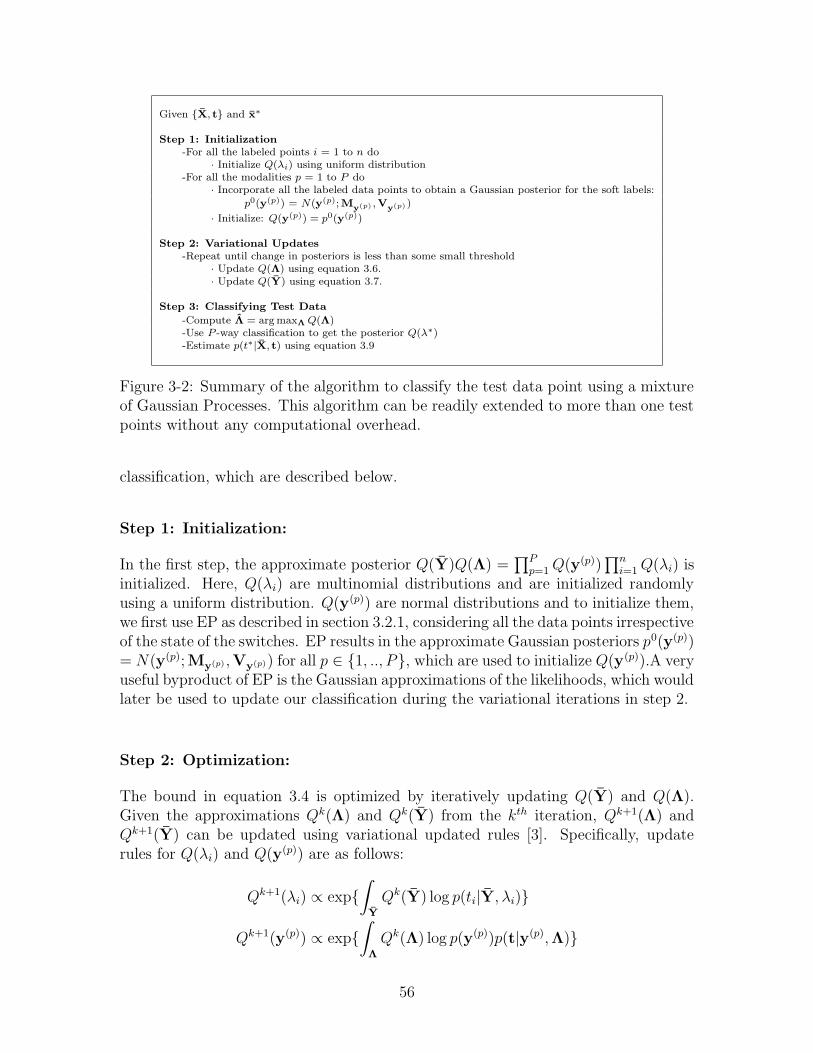
Given {X, t} and x∗

Step 1: Initialization

-For all the labeled points i = 1 to n do· Initialize Q(λi) using uniform distribution

-For all the modalities p = 1 to P do· Incorporate all the labeled data points to obtain a Gaussian posterior for the soft labels:

p0(y(p)) = N(y(p);My(p) ,Vy(p) )

· Initialize: Q(y(p)) = p0(y(p))

Step 2: Variational Updates

-Repeat until change in posteriors is less than some small threshold· Update Q(Λ) using equation 3.6.· Update Q(Y) using equation 3.7.

Step 3: Classifying Test Data

-Compute Λ = arg maxΛ Q(Λ)-Use P -way classification to get the posterior Q(λ∗)-Estimate p(t∗|X, t) using equation 3.9

Figure 3-2: Summary of the algorithm to classify the test data point using a mixtureof Gaussian Processes. This algorithm can be readily extended to more than one testpoints without any computational overhead.

classification, which are described below.

Step 1: Initialization:

In the first step, the approximate posterior Q(Y)Q(Λ) =∏P

p=1Q(y(p))∏n

i=1Q(λi) isinitialized. Here, Q(λi) are multinomial distributions and are initialized randomlyusing a uniform distribution. Q(y(p)) are normal distributions and to initialize them,we first use EP as described in section 3.2.1, considering all the data points irrespectiveof the state of the switches. EP results in the approximate Gaussian posteriors p0(y(p))= N(y(p);My(p) ,Vy(p)) for all p ∈ {1, .., P}, which are used to initialize Q(y(p)).A veryuseful byproduct of EP is the Gaussian approximations of the likelihoods, which wouldlater be used to update our classification during the variational iterations in step 2.

Step 2: Optimization:

The bound in equation 3.4 is optimized by iteratively updating Q(Y) and Q(Λ).Given the approximations Qk(Λ) and Qk(Y) from the kth iteration, Qk+1(Λ) andQk+1(Y) can be updated using variational updated rules [3]. Specifically, updaterules for Q(λi) and Q(y(p)) are as follows:

Qk+1(λi) ∝ exp{

∫

Y

Qk(Y) log p(ti|Y, λi)}

Qk+1(y(p)) ∝ exp{

∫

Λ

Qk(Λ) log p(y(p))p(t|y(p),Λ)}

56

The update for Q(λi = p) can be written as:

Qk+1(λi = p) ∝ exp{

∫

y(p)i

Qk(y(p)i ) log p(ti|y

(p)i )} (3.5)

= exp{

∫

y(p)i

Qk(y(p)i ) log(Φ(tiy

(p)i )} (3.6)

Equation 3.6 is intractable but can be computed efficiently by importance samplingusing the 1-D Gaussian Qk(yp

i ) as a proposal distribution. More importantly, we havethe Gaussian approximations from EP for the likelihood term:

p(ti|y(p)i ) ≈ s

(p)i exp(−

1

2v(p)i

(y(p)i · ti −m

(p)i )2)

It can be shown that the update rule for Q(y(p)) reduces down to:

Qk+1(y(p)) ∝ p(y(p))n

∏

i=1

N(y(p)i ;m

(p)i · ti,

v(p)i

Qk(λi)) (3.7)

This is just a product of Gaussians; thus, there is no need to rerun EP to estimate thenew posterior over soft classifications. Note that Q(λi) divides the variance, hencecontrolling the contribution of each labeled data point for different channels.

Step 3: Classification:

Once we have the posterior over the switches, Q(λi) ∀i ∈ [1..n], we first infer theswitches for the test data x∗ using a meta-level GP based classification system. Forthis, we do a P -way classification using the GP algorithm described in 3.2.1 withΛ = arg maxΛQ(Λ) as labels. Specifically, for an unlabeled point x∗, P differentclassifications are done where each classification provides us with q∗r , the probabilitythat channel r ∈ {1, .., P} was chosen to classify x∗. The posterior Q(λ∗ = r) is thenset to q∗r

∑Pp=1 q∗p

.

In our experiments, to perform this P -way classification, we clubbed all the chan-nels together and used imputation by filling in -1 as observations for the modalitiesthat were missing. We also tried the imputation scheme of filling in 0, but the perfor-mance was slightly worse. Note, that -1 here now represents the state of error in theobservations and the meta-level decision system can take these errors into account tochoose the best modalities for classification. Further, note that we are not limited tousing all the channels clubbed together: various combinations of the modalities canbe used including other indicator and contextual variables.

Once we have the posterior over the switch for the test data, Q(λ∗), we can infer

57

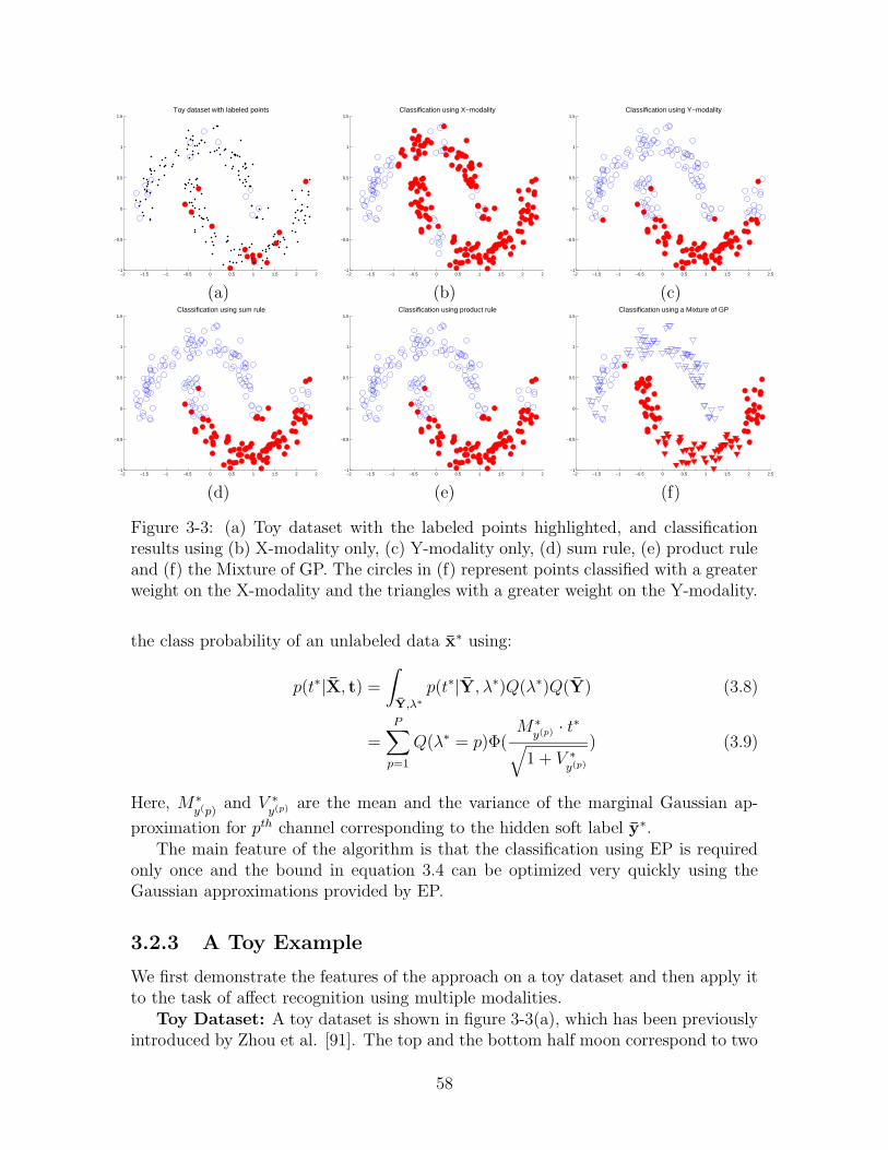
−2 −1.5 −1 −0.5 0 0.5 1 1.5 2 2.5−1

−0.5

0

0.5

1

1.5Toy dataset with labeled points

−2 −1.5 −1 −0.5 0 0.5 1 1.5 2 2.5−1

−0.5

0

0.5

1

1.5Classification using X−modality

−2 −1.5 −1 −0.5 0 0.5 1 1.5 2 2.5−1

−0.5

0

0.5

1

1.5Classification using Y−modality

(a) (b) (c)

−2 −1.5 −1 −0.5 0 0.5 1 1.5 2 2.5−1

−0.5

0

0.5

1

1.5Classification using sum rule

−2 −1.5 −1 −0.5 0 0.5 1 1.5 2 2.5−1

−0.5

0

0.5

1

1.5Classification using product rule

−2 −1.5 −1 −0.5 0 0.5 1 1.5 2 2.5−1

−0.5

0

0.5

1

1.5Classification using a Mixture of GP

(d) (e) (f)

Figure 3-3: (a) Toy dataset with the labeled points highlighted, and classificationresults using (b) X-modality only, (c) Y-modality only, (d) sum rule, (e) product ruleand (f) the Mixture of GP. The circles in (f) represent points classified with a greaterweight on the X-modality and the triangles with a greater weight on the Y-modality.

the class probability of an unlabeled data x∗ using:

p(t∗|X, t) =

∫

Y,λ∗

p(t∗|Y, λ∗)Q(λ∗)Q(Y) (3.8)

=P

∑

p=1

Q(λ∗ = p)Φ(M∗

y(p) · t∗

√

1 + V ∗y(p)

) (3.9)

Here, M ∗y(p)

and V ∗y(p) are the mean and the variance of the marginal Gaussian ap-

proximation for pth channel corresponding to the hidden soft label y∗.The main feature of the algorithm is that the classification using EP is required

only once and the bound in equation 3.4 can be optimized very quickly using theGaussian approximations provided by EP.

3.2.3 A Toy Example

We first demonstrate the features of the approach on a toy dataset and then apply itto the task of affect recognition using multiple modalities.

Toy Dataset: A toy dataset is shown in figure 3-3(a), which has been previouslyintroduced by Zhou et al. [91]. The top and the bottom half moon correspond to two

58

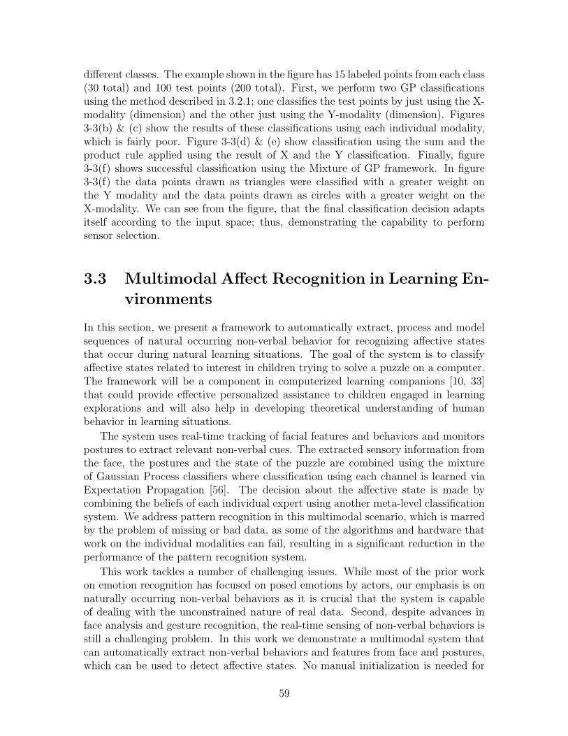
different classes. The example shown in the figure has 15 labeled points from each class(30 total) and 100 test points (200 total). First, we perform two GP classificationsusing the method described in 3.2.1; one classifies the test points by just using the X-modality (dimension) and the other just using the Y-modality (dimension). Figures3-3(b) & (c) show the results of these classifications using each individual modality,which is fairly poor. Figure 3-3(d) & (e) show classification using the sum and theproduct rule applied using the result of X and the Y classification. Finally, figure3-3(f) shows successful classification using the Mixture of GP framework. In figure3-3(f) the data points drawn as triangles were classified with a greater weight onthe Y modality and the data points drawn as circles with a greater weight on theX-modality. We can see from the figure, that the final classification decision adaptsitself according to the input space; thus, demonstrating the capability to performsensor selection.

3.3 Multimodal Affect Recognition in Learning En-

vironments

In this section, we present a framework to automatically extract, process and modelsequences of natural occurring non-verbal behavior for recognizing affective statesthat occur during natural learning situations. The goal of the system is to classifyaffective states related to interest in children trying to solve a puzzle on a computer.The framework will be a component in computerized learning companions [10, 33]that could provide effective personalized assistance to children engaged in learningexplorations and will also help in developing theoretical understanding of humanbehavior in learning situations.

The system uses real-time tracking of facial features and behaviors and monitorspostures to extract relevant non-verbal cues. The extracted sensory information fromthe face, the postures and the state of the puzzle are combined using the mixtureof Gaussian Process classifiers where classification using each channel is learned viaExpectation Propagation [56]. The decision about the affective state is made bycombining the beliefs of each individual expert using another meta-level classificationsystem. We address pattern recognition in this multimodal scenario, which is marredby the problem of missing or bad data, as some of the algorithms and hardware thatwork on the individual modalities can fail, resulting in a significant reduction in theperformance of the pattern recognition system.

This work tackles a number of challenging issues. While most of the prior workon emotion recognition has focused on posed emotions by actors, our emphasis is onnaturally occurring non-verbal behaviors as it is crucial that the system is capableof dealing with the unconstrained nature of real data. Second, despite advances inface analysis and gesture recognition, the real-time sensing of non-verbal behaviors isstill a challenging problem. In this work we demonstrate a multimodal system thatcan automatically extract non-verbal behaviors and features from face and postures,which can be used to detect affective states. No manual initialization is needed for

59

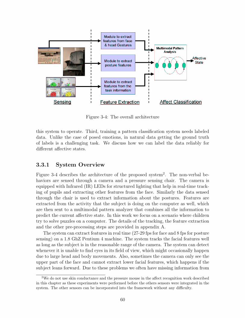
Figure 3-4: The overall architecture

this system to operate. Third, training a pattern classification system needs labeleddata. Unlike the case of posed emotions, in natural data getting the ground truthof labels is a challenging task. We discuss how we can label the data reliably fordifferent affective states.

3.3.1 System Overview

Figure 3-4 describes the architecture of the proposed system2. The non-verbal be-haviors are sensed through a camera and a pressure sensing chair. The camera isequipped with Infrared (IR) LEDs for structured lighting that help in real-time track-ing of pupils and extracting other features from the face. Similarly the data sensedthrough the chair is used to extract information about the postures. Features areextracted from the activity that the subject is doing on the computer as well, whichare then sent to a multimodal pattern analyzer that combines all the information topredict the current affective state. In this work we focus on a scenario where childrentry to solve puzzles on a computer. The details of the tracking, the feature extractionand the other pre-processing steps are provided in appendix A.

The system can extract features in real time (27-29 fps for face and 8 fps for posturesensing) on a 1.8 GhZ Pentium 4 machine. The system tracks the facial features wellas long as the subject is in the reasonable range of the camera. The system can detectwhenever it is unable to find eyes in its field of view, which might occasionally happendue to large head and body movements. Also, sometimes the camera can only see theupper part of the face and cannot extract lower facial features, which happens if thesubject leans forward. Due to these problems we often have missing information from

2We do not use skin conductance and the pressure mouse in the affect recognition work describedin this chapter as these experiments were performed before the others sensors were integrated in thesystem. The other sensors can be incorporated into the framework without any difficulty.

60

the face; thus, we need an affect recognition system that is robust to such trackingfailures.

Table 3.2 shows all the features that are extracted every one eighth of a second.We deliberately grouped them under “channels”, separating for example the upperand lower face features because often the upper face features were present but not thelower. We observe that the cause of any missing feature or bad data is a sensor failureand the features tend to be missing in predictable groups; hence, for the implemen-tation we form four different channels (table 3.2) and each channel corresponds to agroup of features that can go missing simultaneously depending upon which sensorfails. Our strategy will be to fuse decisions from these channels, rather than individualfeatures, thus, preserving some higher order statistics between different features.

Collecting the Database

Data collection for affective studies is a challenging task: The subject needs to beexposed to conditions that can elicit the emotional state in an authentic way; if weelicit affective states on demand, it is almost guaranteed not to bring out genuinely therequired emotional state. Affective states associated with interest and boredom wereelicited through an experiment with children aged 8 to 11 years, coming from relativelyaffluent areas of the state of Massachusetts in the USA. Each child was asked to solvea constraint satisfaction game called Fripples Place for approximately 20 minutesand the space where the experiment took place was a naturalistic setting allowingthe subject to move freely. It was arranged with the sensor chair, one computerplaying the game and recording the screen activity, having a monitor, standard mouseand keyboard, as well as two video-cameras: one capturing a side-view and one thefrontal view; and finally, a Blue Eyes camera capturing the face. We made the camerasunobtrusive to encourage natural responses preserving as much as possible the originalbehavior. Given that we cannot directly observe the student’s internal thoughts andemotions, nor can children in the age range of 8 and 11 years old reliably articulatetheir feelings, we chose to obtain labels of affective states from observers who are

Table 3.2: Extracted features from different modalities which are grouped into chan-nels.

Channel 1: Upper Face

Brow ShapeEye Shape

likelihood of nodlikelihood of shakelikelihood of blink

Channel 3: Posture

Current PostureLevel of Activity

Channel 2: Lower Face

Probability of FidgetProbability of Smile

Channel 4: Game

Level of DifficultyState of the Game

61

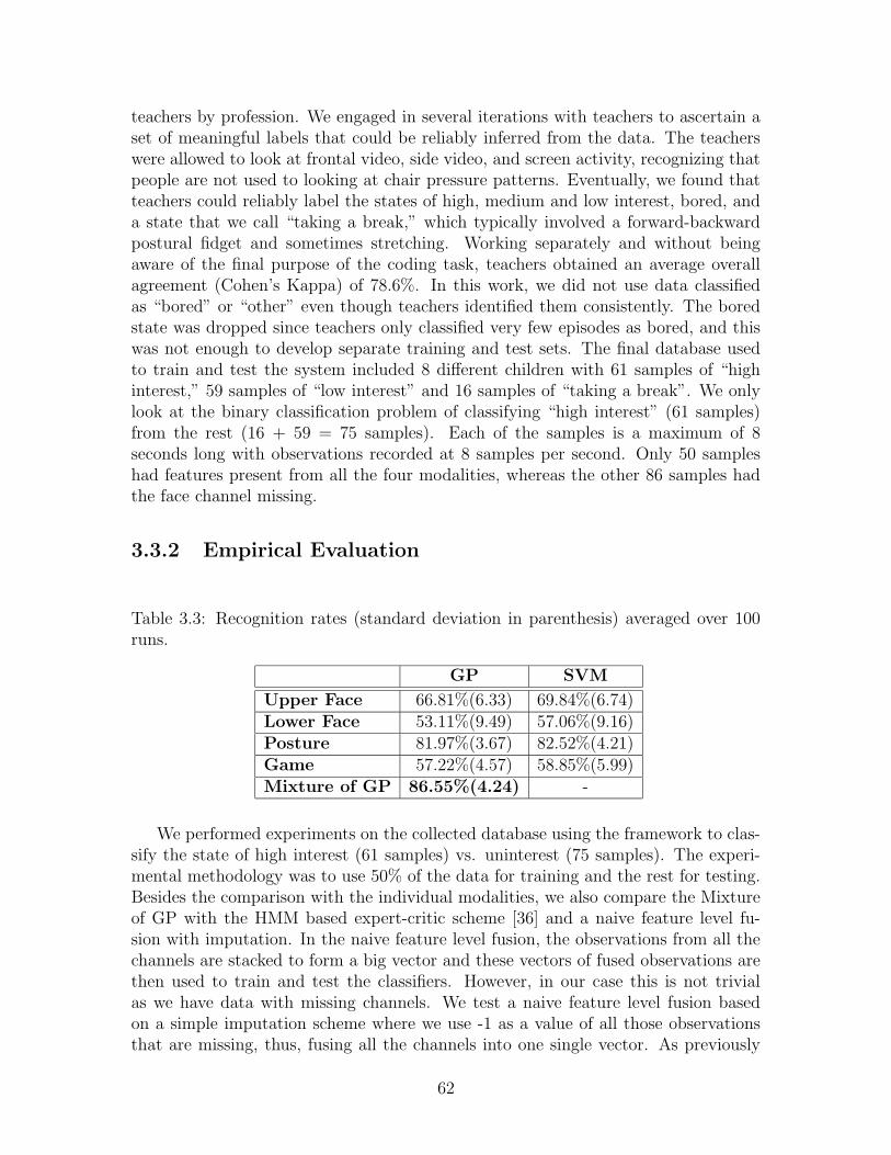
teachers by profession. We engaged in several iterations with teachers to ascertain aset of meaningful labels that could be reliably inferred from the data. The teacherswere allowed to look at frontal video, side video, and screen activity, recognizing thatpeople are not used to looking at chair pressure patterns. Eventually, we found thatteachers could reliably label the states of high, medium and low interest, bored, anda state that we call “taking a break,” which typically involved a forward-backwardpostural fidget and sometimes stretching. Working separately and without beingaware of the final purpose of the coding task, teachers obtained an average overallagreement (Cohen’s Kappa) of 78.6%. In this work, we did not use data classifiedas “bored” or “other” even though teachers identified them consistently. The boredstate was dropped since teachers only classified very few episodes as bored, and thiswas not enough to develop separate training and test sets. The final database usedto train and test the system included 8 different children with 61 samples of “highinterest,” 59 samples of “low interest” and 16 samples of “taking a break”. We onlylook at the binary classification problem of classifying “high interest” (61 samples)from the rest (16 + 59 = 75 samples). Each of the samples is a maximum of 8seconds long with observations recorded at 8 samples per second. Only 50 sampleshad features present from all the four modalities, whereas the other 86 samples hadthe face channel missing.

3.3.2 Empirical Evaluation

Table 3.3: Recognition rates (standard deviation in parenthesis) averaged over 100runs.

GP SVM

Upper Face 66.81%(6.33) 69.84%(6.74)Lower Face 53.11%(9.49) 57.06%(9.16)Posture 81.97%(3.67) 82.52%(4.21)Game 57.22%(4.57) 58.85%(5.99)Mixture of GP 86.55%(4.24) -

We performed experiments on the collected database using the framework to clas-sify the state of high interest (61 samples) vs. uninterest (75 samples). The experi-mental methodology was to use 50% of the data for training and the rest for testing.Besides the comparison with the individual modalities, we also compare the Mixtureof GP with the HMM based expert-critic scheme [36] and a naive feature level fu-sion with imputation. In the naive feature level fusion, the observations from all thechannels are stacked to form a big vector and these vectors of fused observations arethen used to train and test the classifiers. However, in our case this is not trivialas we have data with missing channels. We test a naive feature level fusion basedon a simple imputation scheme where we use -1 as a value of all those observationsthat are missing, thus, fusing all the channels into one single vector. As previously

62

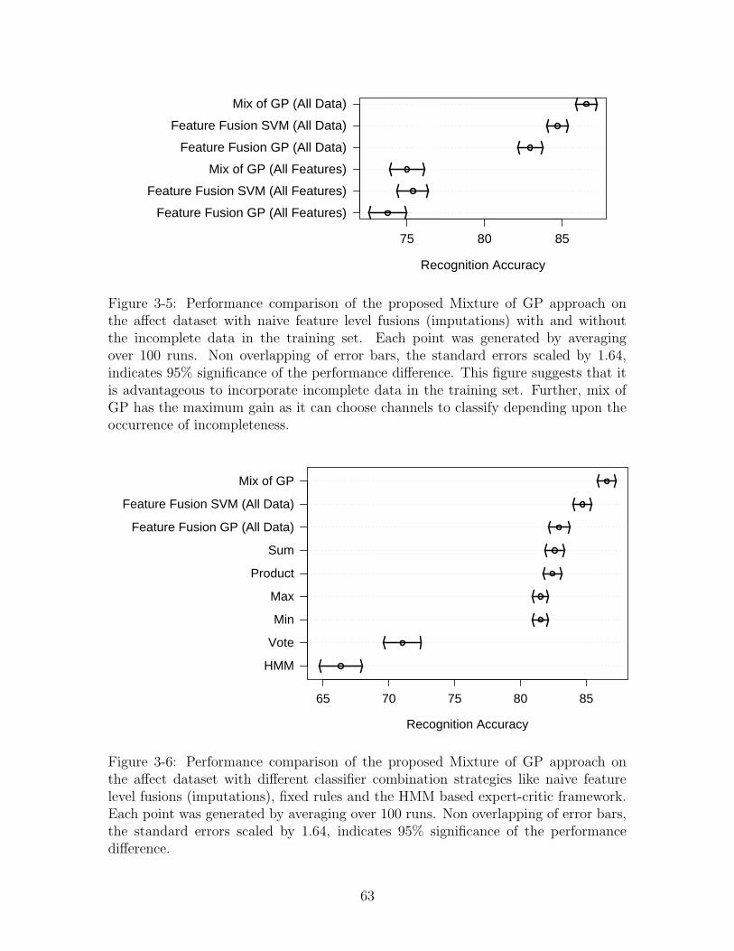
Feature Fusion GP (All Features)

Feature Fusion SVM (All Features)

Mix of GP (All Features)

Feature Fusion GP (All Data)

Feature Fusion SVM (All Data)

Mix of GP (All Data)

75 80 85

Recognition Accuracy

Figure 3-5: Performance comparison of the proposed Mixture of GP approach onthe affect dataset with naive feature level fusions (imputations) with and withoutthe incomplete data in the training set. Each point was generated by averagingover 100 runs. Non overlapping of error bars, the standard errors scaled by 1.64,indicates 95% significance of the performance difference. This figure suggests that itis advantageous to incorporate incomplete data in the training set. Further, mix ofGP has the maximum gain as it can choose channels to classify depending upon theoccurrence of incompleteness.

HMM

Vote

Min

Max

Product

Sum

Feature Fusion GP (All Data)

Feature Fusion SVM (All Data)

Mix of GP

65 70 75 80 85

Recognition Accuracy

Figure 3-6: Performance comparison of the proposed Mixture of GP approach onthe affect dataset with different classifier combination strategies like naive featurelevel fusions (imputations), fixed rules and the HMM based expert-critic framework.Each point was generated by averaging over 100 runs. Non overlapping of error bars,the standard errors scaled by 1.64, indicates 95% significance of the performancedifference.

63

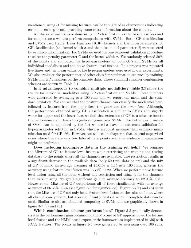
mentioned, using -1 for missing features can be thought of as observations indicatingerrors in sensing; hence, providing some extra information about the context.

All the experiments were done using GP classification as the base classifiers andfor completeness we also perform comparisons with SVMs. Both, GP classificationand SVMs used Radial Basis Function (RBF) kernels and the hyperparameters forGP classification (the kernel width σ and the noise model parameter β) were selectedby evidence maximization. For SVMs we used the leave-one-out validation procedureto select the penalty parameter C and the kernel width σ. We randomly selected 50%of the points and computed the hyper-parameters for both GPs and SVMs for allindividual modalities and the naive feature level fusions. This process was repeatedfive times and the mean values of the hyperparameters were used in our experiments.We also evaluate the performance of other classifier combination schemes by trainingSVMs and GP classifiers on the complete data. These standard classifier combinationschemes are shown in Table 3.1.

Is it advantageous to combine multiple modalities? Table 3.3 shows theresults for individual modalities using GP classification and SVMs. These numberswere generated by averaging over 100 runs and we report the mean and the stan-dard deviation. We can see that the posture channel can classify the modalities best,followed by features from the upper face, the game and the lower face. Although,the performance obtained using GP classification is similar to SVMs and slightlyworse for upper and the lower face, we find that extension of GP to a mixture booststhe performance and leads to significant gains over SVMs. The better performanceof SVMs can be explained by the fact we used a leave-one-out cross validation forhyperparameter selection in SVMs, which is a robust measure than evidence maxi-mization used for GP [66]. However, we will see in chapter 4 that in semi-supervisedcases where there are very few labeled data points available evidence maximizationmight be preferable.

Does including incomplete data in the training set help? We comparethe Mixture of GP to feature level fusion while restricting the training and testingdatabase to the points where all the channels are available. The restriction results ina significant decrease in the available data (only 50 total data points) and the mixof GP obtained an average accuracy of 75.01% ± 1.15 over 100 runs, whereas theaccuracy using feature level fusion was 73.77%±1.22. When we perform naive featurelevel fusion using all the data, without any restriction and using -1 for the channelsthat were missing, we get a significant gain in average accuracy to 82.93%±0.81.However, the Mixture of GP outperforms all of these significantly with an averageaccuracy of 86.55%±0.55 (see figure 3-5 for significance). Figure 3-7(a) and (b) showthat the Mixture of GP not only beats feature level fusion on the subset of data whereall channels are present, but also significantly beats it when incomplete data can beused. Similar results are obtained comparing to SVMs and are graphically shown infigure 3-7 (c) and (d).

Which combination scheme performs best? Figure 3-5 graphically demon-strates the performance gain obtained by the Mixture of GP approach over the featurelevel fusions and the HMM based expert critic framework as implemented in [36] withFACS features. The points in figure 3-5 were generated by averaging over 100 runs.

64

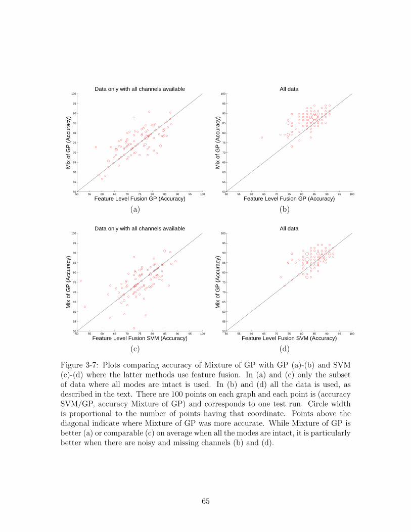
50 55 60 65 70 75 80 85 90 95 10050

55

60

65

70

75

80

85

90

95

100

Mix

of G

P (

Acc

urac

y)

Feature Level Fusion GP (Accuracy)

Data only with all channels available

50 55 60 65 70 75 80 85 90 95 10050

55

60

65

70

75

80

85

90

95

100

Mix

of G

P (

Acc

urac

y)

Feature Level Fusion GP (Accuracy)

All data

(a) (b)

50 55 60 65 70 75 80 85 90 95 10050

55

60

65

70

75

80

85

90

95

100

Mix

of G

P (

Acc

urac

y)

Feature Level Fusion SVM (Accuracy)

Data only with all channels available

50 55 60 65 70 75 80 85 90 95 10050

55

60

65

70

75

80

85

90

95

100

Mix

of G

P (

Acc

urac

y)

Feature Level Fusion SVM (Accuracy)

All data

(c) (d)

Figure 3-7: Plots comparing accuracy of Mixture of GP with GP (a)-(b) and SVM(c)-(d) where the latter methods use feature fusion. In (a) and (c) only the subsetof data where all modes are intact is used. In (b) and (d) all the data is used, asdescribed in the text. There are 100 points on each graph and each point is (accuracySVM/GP, accuracy Mixture of GP) and corresponds to one test run. Circle widthis proportional to the number of points having that coordinate. Points above thediagonal indicate where Mixture of GP was more accurate. While Mixture of GP isbetter (a) or comparable (c) on average when all the modes are intact, it is particularlybetter when there are noisy and missing channels (b) and (d).

65

FACS

Lower Face

Upper Face

55 60 65

Recognition Accuracy

HMM

Mix of GP (FACS)

Mix of GP

65 70 75 80 85

Recognition Accuracy

(a) (b)

Figure 3-8: (a) Comparison of the recognition accuracy obtained while performingGP classification using the automatically extracted features from the lower and upperface with the accuracy obtained using manually coded Facial AUs. (b) Comparisonof the recognition accuracy obtained by the Mixture of GP that uses automaticallyextracted facial features with Mixture of GP approach that uses manual FACS codingof AUs and the expert-critic HMM framework. Each point was generated by averagingover 100 runs with random 50-50 training and testing split. Non overlapping of errorbars, the standard errors scaled by 1.64, indicates 95% significance of the performancedifference.

The non-overlapping error bars, standard errors scaled by 1.64, signify 95% confidencein performance difference. The Mixture of GP uses all the data and can handle themissing information better than naive fusion methods; thus, it provides a significantperformance boost.

FACS vs. automatically extracted features. In our earlier work [36, 32], wehad used manually encoded FACS based Action Units (AU) as features extracted fromthe face. Figure 3-8(a) shows the improvement in performance obtained by using thefeatures extracted from lower and upper face as described in section A.1. The accu-racy of 66.81 ± 6.33 obtained while performing GP classification with automaticallyextracted upper facial features was significantly better than the accuracy of 54.19 ±3.79 obtained with GP classification that used the manually coded upper AUs. Also,from figure 3-8(b) we can see that similar gains are observed when using the Mixtureof GPs framework with the automatically extracted features. The difference is dueto two factors. First, the set of automatically extracted upper facial features is richerthan the AUs. Second, the AUs were manually encoded by just one FACS expert,thus, resulting in features prone to noise.

3.4 Conclusions and Future Work

In this chapter, we proposed a unified approach using a mixture of Gaussian Processesfor achieving sensor fusion under the challenging conditions of missing channels. Theincompleteness due to missing features is handled by combining the decisions of ex-perts trained on subsets of features, where the decision fusion ignores the classifiersthat act on the missing features. We provide an algorithm for Bayesian inference de-signed with a fast update of classification decisions based on variational and Gaussianapproximations. On the task of classifying affective state of interest using informa-tion from face, postures and task information, the Mixture of GP method outperforms

66

feature level fusion based on imputation and several standard classifier combinationschemes and obtained a recognition rate of 86%. Further, we also demonstrated thatthere are significant gains when the incomplete data is incorporated in the trainingset.

Future work includes incorporation of active learning and application of this frame-work to other challenging problems with limited labeled data. Note, that we pre-selected the subsets of features for the Mixture of GP framework and the subsetswere mutually exclusive. However, the features across different modalities can becorrelated and it can be advantageous to look at the subsets of features from differentmodalities where these subsets can even be overlapping. A direction for the futurewould be to discover these sets automatically. Further, there are interesting possibil-ities where the Mixture of GPs model is combined with different noise-models, semi-supervised classification and other extensions proposed in these thesis. Finally, thereare many applications in different domains such as sensor networks, social networksand other multimodal scenarios where the proposed method can be used effectively.

67

68

Chapter 4

Gaussian Process Classificationwith Partially Labeled Data

Often in machine learning1 problems there are a large number of data points of whichfew are labeled. This usually happens as it might be very expensive or difficult toobtain the labels. The incompleteness resulting from partially labeled data has beenwell researched and is often referred to as semi-supervised classification. Specifically,given a set of data points, among which few are labeled, the goal in semi-supervisedlearning is to predict the labels of the unlabeled points using the complete set of datapoints. By looking at both the labeled and the unlabeled data, the learning algorithmcan exploit the distribution of data points to learn the classification boundary.

The original Gaussian process formulation cannot be directly used to exploit theinformation from the unlabeled data. This point has been elaborated earlier by Seeger[74] and more recently by Lawrence and Jordan [48]. The GP prior just encodes theassumption that similar data points should have the same label and itself does notcontain any information about the data distribution. Further, the likelihood termonly incorporates information from the labeled data; thus, the traditional Gaussianprocess classification cannot be trivially extended to the semi-supervised scenario.

Lawrence and Jordan [48] proposed to overcome this problem by introducing thenull category noise model. The idea behind this approach is to use the unlabeled datato steer the decision boundary to the region of low data density. Specifically, theypropose to modify the likelihood such that the model imitates the SVM loss functionand favors the decision boundary with large margins. Now, the algorithm can alsolook at the unlabeled data points and exploit the information from the distributionof the data points to find the solution.

The work presented here explores other alternatives besides the null category noisemodel. Specifically, rather than focusing on the noise model, we aim to study theextensions of the standard Gaussian process prior by introducing regularization basedon the unlabeled and the labeled data points. We focus mainly on graph based semi-supervised classification techniques, where the key idea is to exploit the notion ofsimilarity to label the unlabeled points. Given a set of labeled and unlabeled points,

1The work described in this chapter appears in Neural Information Processing Systems, 2005 [37]

69

these approaches provide a way to regularize the solution using a similarity graphover the data points. Smola and Kondor [79] have provided a unifying view of manyof these approaches using the theory of Reproducing Kernel Hilbert Space. Moreover,Zhu et al. [94] have also made connections between Gaussian process classificationand semi-supervised learning work based on harmonic functions and Gaussian fields[92]. Similarly, there is recent work in semi-supervised learning that uses ideas be-hind manifold regularization in a Gaussian process framework [78]. This chapter aimsto provide a Bayesian perspective to unify many graph-based semi-supervised clas-sification methods; thus, providing a framework to analyze the similarities and thedifferences among most of the graph based semi-supervised methods.

One of the main problems with many of the existing graph based semi-supervisedclassification techniques is that of hyperparameter learning: performance dependsgreatly on the hyperparameters of the similarity graph, transformation of the graphLaplacian and the noise model. Figure 4 graphically shows this problem. In thisexample, we use an RBF kernel with the parameter σ to measure similarity betweentwo data points. The figures show results using a recent graph based algorithm (LLGC[91]) and as we can see the results can be quite different for different values of thehyperparameter σ. Finding a correct set of hyperparameters is critical for the graphbased methods to work well.

There are many advantages of viewing semi-supervised learning methods from theBayesian perspective. Evidence maximization provides an elegant framework to domodel selection and we provide a way to learn the kernel and hyperparameters forgraph based semi-supervised classification, while adhering to a Bayesian framework.

We exploit the Bayesian framework for learning hyperparameters for graph-basedsemi-supervised classification. Given some labeled data, which can contain inaccu-rate labels, we pose the semi-supervised classification as an inference problem overthe unknown labels. We use the evidence to simultaneously tune the hyperparame-ters that define the structure of the similarity graph, the parameters that determinethe transformation of the graph Laplacian, and any other parameters of the model.Closest to our work is Zhu et al. [94], where they proposed a Laplace approximationfor learning the edge weights. We use Expectation Propagation (EP) for approximateBayesian inference that provides better approximations than Laplace. An additionalcontribution is an EM algorithm to learn the hyperparameters for the edge weights,the parameters of the transformation of the graph spectrum. More importantly, weexplicitly model the level of label noise in the data, while [94] does not do. We providewhat may be the first comparison of hyperparameter learning with cross-validationon state of the art algorithms (LLGC [91] and harmonic fields [92]).

This chapter is organized as follow: First, we mention some existing approachesand ideas that aim to address semi-supervised classification. Followed by that, wedescribe the proposed framework, the hyperparameter learning procedure and alsodiscuss extensions to classify new unseen points that were not part of either the labeledor unlabeled data used in the Bayesian inference. After that, we describe experimentalevaluation and discuss connections of the proposed framework to Gaussian processesand some of the recent work on graph-based semi-supervised classification. We endthe chapter with discussion and a summary.

70

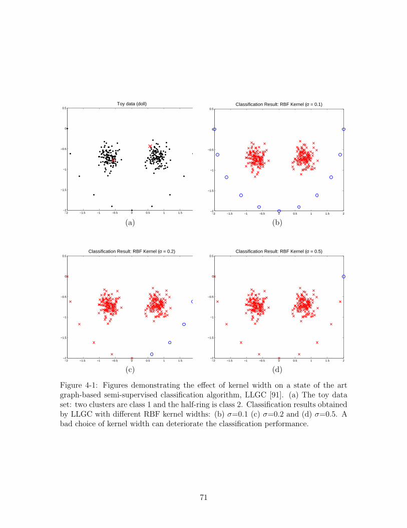
−2 −1.5 −1 −0.5 0 0.5 1 1.5 2−2

−1.5

−1

−0.5

0

0.5Toy data (doll)

−2 −1.5 −1 −0.5 0 0.5 1 1.5 2−2

−1.5

−1

−0.5

0

0.5Classification Result: RBF Kernel (σ = 0.1)

(a) (b)

−2 −1.5 −1 −0.5 0 0.5 1 1.5 2−2

−1.5

−1

−0.5

0

0.5Classification Result: RBF Kernel (σ = 0.2)

−2 −1.5 −1 −0.5 0 0.5 1 1.5 2−2

−1.5

−1

−0.5

0

0.5Classification Result: RBF Kernel (σ = 0.5)

(c) (d)

Figure 4-1: Figures demonstrating the effect of kernel width on a state of the artgraph-based semi-supervised classification algorithm, LLGC [91]. (a) The toy dataset: two clusters are class 1 and the half-ring is class 2. Classification results obtainedby LLGC with different RBF kernel widths: (b) σ=0.1 (c) σ=0.2 and (d) σ=0.5. Abad choice of kernel width can deteriorate the classification performance.

71

4.1 Previous Work

4.1.1 Semi-supervised Classification

There have been a large number of approaches proposed in recent years for semi-supervised learning. The spectrum of the approaches spans generative models, sup-port vector machines (SVMs), graph-based techniques, co-training, information regu-larization etc. Here, we attempt to cover a few of these approaches and the conceptsbehind them.

Generative Models: First, there have been a lot of work on semi-supervised learningbased on a generative paradigm of classification using EM [61]. The idea behind theseapproaches is that the labels corresponding to the unlabeled points are considered ashidden data and the method iterates between estimating these hidden labels andrefining the decision boundary. One of the main drawbacks of these approaches isthat first these methods require a large database to perform well. Second, there hasbeen evidence [12, 15] that the semi-supervised methods might perform poorly whenthe data deviates from the model assumptions (such as Gaussianity).

Transductive SVMs and Related Approaches: One of the more prominentapproaches for semi-supervised classification from the perspective of discriminativemodeling has been the transductive SVM [86]. This approach is explicitly based onthe assumption that the decision boundary lies in the region where the data den-sity is low. Transductive SVMs extend the regular SVM formulation to incorporatethe information from the unlabeled data points, such that the decision boundary issteered away from the region of high density. There have been many successful appli-cations that uses Transductive SVMs. Recently, Lawrence and Jordan [48] proposeda Bayesian approach that can be considered as a Bayesian counterpart to the Trans-ductive SVMs. The approach suggests a null category noise model, which imitates therole of SVM hinge loss by penalizing the decision boundaries that lie in a high densityregion. Both of these methods utilize a noise model to achieve the semi-supervisedclassification. Specifically, the assumption that the decision boundary lies in a regionof low density guides both of these algorithms that, as we will see, is different thanthe assumptions used in graph based semi-supervised classification techniques.

Regularization on Graphs: Many of the approaches proposed recently are veryclosely connected and are either implicitly or explicitly based on regularization ongraphs [79]. The key idea behind these methods is similarity. Essentially, the idea isto put a smoothness constraint on the labels of the data points, such that the pointsthat are similar and lie on the same structure are likely to have the same label. Thesmoothness constraint is obtained by creating a graph with the labeled and unlabeleddata points as the vertices and with edge weights encoding the similarity between thedata points. The semi-supervised classification problem is usually formulated as anoptimization function where the goal is to obtain a labeling of the vertices that isboth smooth over the graph and consistent with the labeled data. This optimizationhas been carried out using a number of different techniques such as, graph mincuts[6] and Tikhonov regularization [4, 5], and the objective to be optimized is basedon analogies drawn from random walks [52, 91], electric networks [92] and spectral

72

methods [31]. Some of the work on semi-supervised learning has proposed kernels[5, 11, 42], which are motivated based on regularization on graphs and can be usedin any kernel based learning algorithm.Other Methods: There are approaches such as co-training [7], information regular-ization [82] and tree based Bayes [38]. The idea behind co-training is to iterativelytrain a pair of classifiers based on features which are assumed to be conditionallyindependent given the class label. Specifically, each classifier “co-trains” the otherclassifier by labeling the unlabeled points. Seeger [74] has mentioned connections ofco-training to the input dependent regularization. Information regularization [14, 82]exploits the assumption that it is more likely for the data points in the regions of highdata density to have the same labels. In the tree based Bayes method [38] the idea isto induce similarities based on evolutionary trees. Specifically, two data points, whichare represented within a tree, are similar if they lie closer in the tree. This approachcan be considered a specific case of the input-dependent regularization.

We limit the scope of our work to the graph based semi-supervised classificationonly. Note, that in all of the graph based methods the smoothness constraint overthe labels depends highly upon the input examples (both labeled and unlabeled)leading to input dependent regularization.This is very different from the traditionaltransductive SVMs as well as the approach proposed by Lawrence and Jordan [48],where there is no input dependent regularization.

4.1.2 Hyperparameter and Kernel Learning

The performance of most of the graph-based algorithms depends upon the edgeweights of the graph, which correspond to the similarity between the vertices. Thenotion of similarity is captured using a kernel matrix and the performance is highlydependent upon the hyper-parameters that describe the kernel. Further, often thesmoothness constraints on the labels are imposed using a transformation of the graphLaplacian [79] and the parameters of the transformation affect the performance. Fi-nally, there might be other parameters in the model, such as parameters to addresslabel noise in the data. Finding a right set of parameters is a challenge, and usuallythe method of choice is cross-validation, which can be prohibitively expensive forreal-world problems and problematic when we have few labeled data points.

The hyperparameter learning is a hard problem. Most of the methods ignore theproblem of learning hyperparameters that determine the similarity graph and thereare only a few approaches that address this problem. Zhu et al. [93] propose anapproach based on semi-definite programming that learns a non-parametric transfor-mation of the graph Laplacians using kernel alignment. This approach assumes thatthe similarity graph is already provided; thus, it does not address the learning ofedge weights. Other approaches include the average label entropy [92] and the useof evidence-maximization using the Laplace approximation [94]. Our work is closelyrelated to Zhu et al. [94]. The main differences are that we use EP to approximate themodel evidence and EM to learn all the hyperparameters. The approximations usingEP has been shown to be better than the Laplace approximation for the purposeof GP classification [45]; thus, providing a significant advantage over the previous

73

method. We describe our method next.

4.2 Bayesian Semi-Supervised Learning

We assume that we are given a set of data points X = {x1, ..,xn+m}, of which XL

= {x1, ..,xn} are labeled as tL = {t1, .., tn} and XU = {xn+1, ..,xn+m} are unlabeled.Throughout this chapter we limit ourselves to two-way classification, thus t ∈ {−1, 1}.Our model assumes that the hard labels ti depend upon hidden soft-labels yi for all i.Given the dataset D = [{XL, tL},XU ], the task of semi-supervised learning is then toinfer the posterior p(tU |D), where tU = [tn+1, .., tn+m]. The posterior can be writtenas:

p(tU |D) =

∫

y

p(tU |y)p(y|D) (4.1)

In this work, we propose to first approximate the posterior p(y|D) and then use (4.1)to classify the unlabeled data. Using the Bayes rule we can write:

p(y|D) = p(y|X, tL) ∝ p(y|X)p(tL|y)

The term, p(y|X) is the prior. It enforces a smoothness constraint and dependsupon the underlying data manifold. Similar to the spirit of graph regularization [79]we use similarity graphs and their transformed Laplacian to induce priors on the softlabels y. The second term, p(tL|y) is the likelihood that incorporates the informationprovided by the labels.

In this work, p(y|D) is inferred using Expectation Propagation, a technique forapproximate Bayesian inference [56]. Note, that similar formulation has also beenproposed by Sindhwani et al. [78]. In the following subsections first we describe theprior and the likelihood in detail and then we show how evidence maximization canbe used to learn hyperparameters and other parameters in the model.

4.2.1 Priors and Regularization on Graphs

The prior plays a significant role in semi-supervised learning, especially when thereis only a small amount of labeled data. The prior imposes a smoothness constraintand should be such that it gives higher probability to the labelings that respect thesimilarity of the graph.

The prior, p(y|X), is constructed by first forming an undirected graph over thedata points. The data points are the nodes of the graph and edge-weights betweenthe nodes are based on similarity. This similarity is usually captured using a kernel.Examples of kernels include RBF, polynomial etc. Given the data points and a kernel,we can construct an (n + m) × (n + m) kernel matrix K, where Kij = k(xi,xj) forall i ∈ {1, .., n+m}.

Lets consider the matrix K, which is same as the matrix K, except that thediagonals are set to zero. Further, if G is a diagonal matrix with the diagonal entries

74

Gii =∑

j Kij, then we can construct the combinatorial Laplacian (∆ = G − K)

or the normalized Laplacian (∆ = I − G− 12 KG− 1

2 .) of the graph. For brevity, inthe text we use ∆ as a notation for both the Laplacians. Both the Laplacians aresymmetric and positive semidefinite. Consider the eigen decomposition of ∆ where{vi} denote the eigenvectors and {λi} the corresponding eigenvalues; thus, we canwrite ∆ =

∑n+mi=1 λiviv

Ti . Usually, a transformation r(∆) =

∑n+mi=1 r(λi)viv

Ti that

modifies the spectrum of ∆ is used as a regularizer. Specifically, the smoothnessimposed by this regularizer prefers soft labeling for which the norm yT r(∆)y is small.Equivalently, we can interpret this probabilistically as following:

p(y|X) ∝ e−12yT r(∆)y = N(0, r(∆)−1) (4.2)

Where r(∆)−1 denotes the pseudo-inverse if the inverse does not exist. Equation(4.2) suggests that the labelings with the small value of yT r(∆)y are more probablethan the others. Note, that when r(∆) is not invertible the prior is improper. Thefact that the prior can be written as a Gaussian is advantageous as techniques forapproximate inference can be easily applied. Also, different choices of transforma-tion functions lead to different semi-supervised learning algorithms. For example,the approach based on Gaussian fields and harmonic functions (Harmonic) [92] canbe thought of as using the transformation r(λ) = λ on the combinatorial Laplacianwithout any noise model. Similarly, the approach based in local and global consis-tency (LLGC) [91] can be thought of as using the same transformation but on thenormalized Laplacian and a Gaussian likelihood. Therefore, it is easy to see thatmost of these algorithms can exploit the proposed evidence maximization framework.In the following we focus only on the parametric linear transformation r(λ) = λ+ δ.Note that this transformation removes zero eigenvalues from the spectrum of ∆.

4.2.2 The Likelihood

Assuming conditional independence of the observed labels given the hidden soft labels,the likelihood p(tL|y) can be written as p(tL|y) =

∏ni=1 p(ti|yi). The likelihood models

the probabilistic relation between the observed label ti and the hidden label yi. Manyreal-world datasets contain hand-labeled data and can often have labeling errors.While most people tend to model label errors with a linear or quadratic slack inthe likelihood, it has been noted that such an approach does not address the caseswhere label errors are far from the decision boundary [39]. The flipping likelihood canhandle errors even when they are far from the decision boundary and can be writtenas:

p(ti|yi) = ε(1 − Φ(yi · ti)) + (1 − ε)Φ(yi · ti) = ε+ (1 − 2ε)Φ(yi · ti) (4.3)

Here, Φ is the step function, ε is the labeling error rate and the model admits pos-sibility of errors in labeling with a probability ε. This likelihood has been earlierused in the context of Gaussian process classification [39, 63]. The above describedlikelihood explicitly models the labeling error rate; thus, the model should be more

75

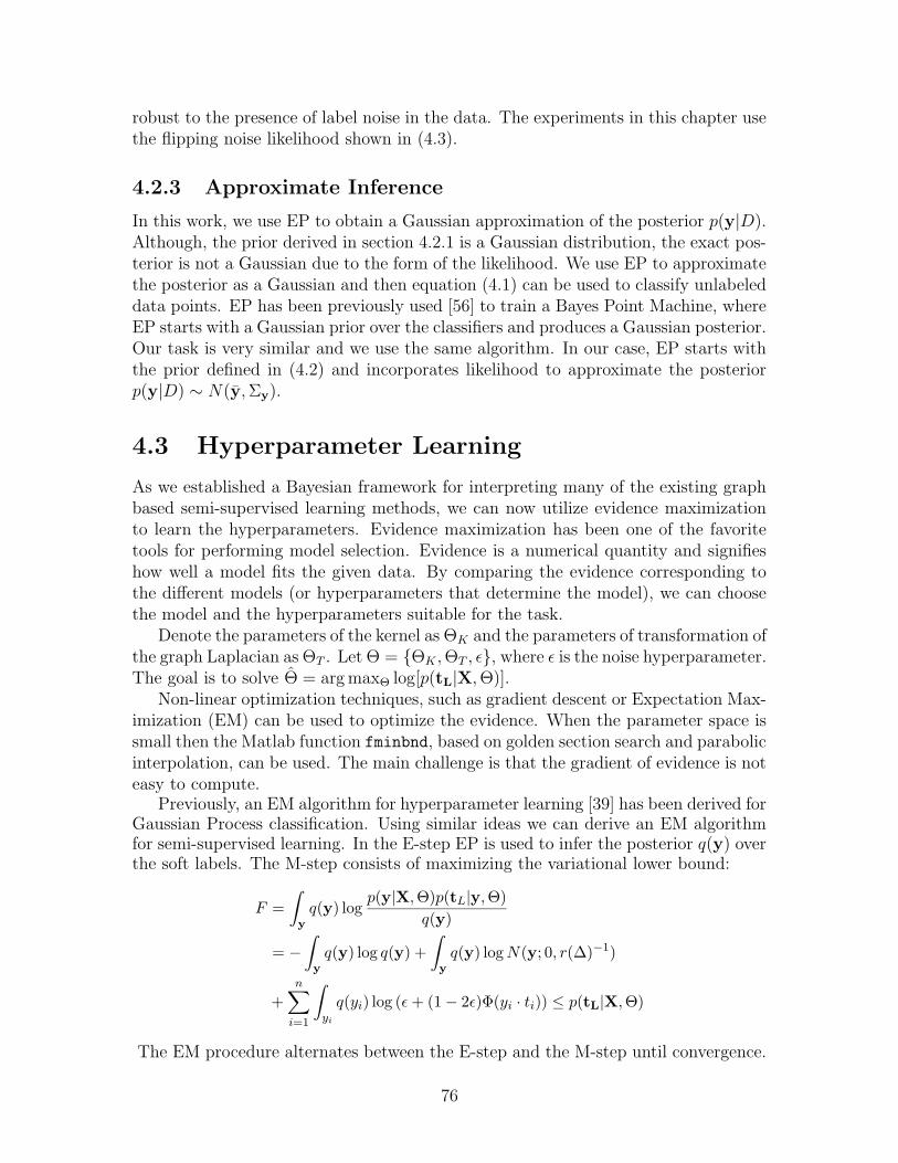
robust to the presence of label noise in the data. The experiments in this chapter usethe flipping noise likelihood shown in (4.3).

4.2.3 Approximate Inference

In this work, we use EP to obtain a Gaussian approximation of the posterior p(y|D).Although, the prior derived in section 4.2.1 is a Gaussian distribution, the exact pos-terior is not a Gaussian due to the form of the likelihood. We use EP to approximatethe posterior as a Gaussian and then equation (4.1) can be used to classify unlabeleddata points. EP has been previously used [56] to train a Bayes Point Machine, whereEP starts with a Gaussian prior over the classifiers and produces a Gaussian posterior.Our task is very similar and we use the same algorithm. In our case, EP starts withthe prior defined in (4.2) and incorporates likelihood to approximate the posteriorp(y|D) ∼ N(y,Σy).

4.3 Hyperparameter Learning

As we established a Bayesian framework for interpreting many of the existing graphbased semi-supervised learning methods, we can now utilize evidence maximizationto learn the hyperparameters. Evidence maximization has been one of the favoritetools for performing model selection. Evidence is a numerical quantity and signifieshow well a model fits the given data. By comparing the evidence corresponding tothe different models (or hyperparameters that determine the model), we can choosethe model and the hyperparameters suitable for the task.

Denote the parameters of the kernel as ΘK and the parameters of transformation ofthe graph Laplacian as ΘT . Let Θ = {ΘK ,ΘT , ε}, where ε is the noise hyperparameter.The goal is to solve Θ = arg maxΘ log[p(tL|X,Θ)].

Non-linear optimization techniques, such as gradient descent or Expectation Max-imization (EM) can be used to optimize the evidence. When the parameter space issmall then the Matlab function fminbnd, based on golden section search and parabolicinterpolation, can be used. The main challenge is that the gradient of evidence is noteasy to compute.

Previously, an EM algorithm for hyperparameter learning [39] has been derived forGaussian Process classification. Using similar ideas we can derive an EM algorithmfor semi-supervised learning. In the E-step EP is used to infer the posterior q(y) overthe soft labels. The M-step consists of maximizing the variational lower bound:

F =

∫

y

q(y) logp(y|X, Θ)p(tL|y, Θ)

q(y)

= −

∫

y

q(y) log q(y) +

∫

y

q(y) log N(y; 0, r(∆)−1)

+n

∑

i=1

∫

yi

q(yi) log (ε + (1 − 2ε)Φ(yi · ti)) ≤ p(tL|X, Θ)

The EM procedure alternates between the E-step and the M-step until convergence.

76

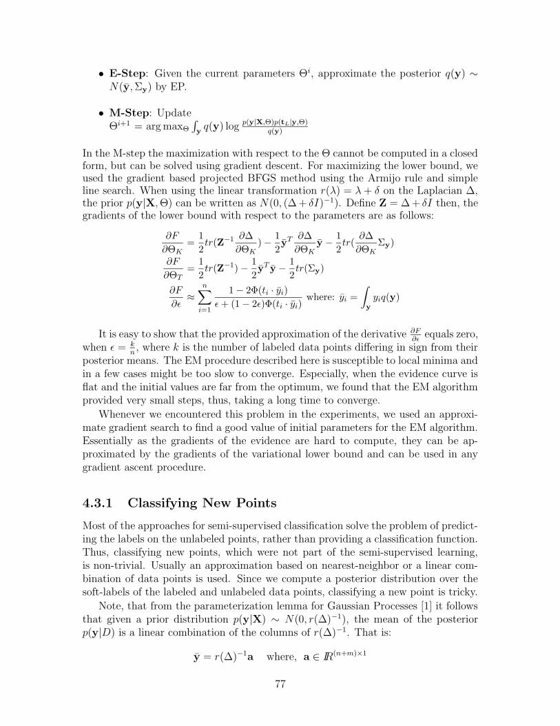
• E-Step: Given the current parameters Θi, approximate the posterior q(y) ∼N(y,Σy) by EP.

• M-Step: UpdateΘi+1 = arg maxΘ

∫

yq(y) log p(y|X,Θ)p(tL|y,Θ)

q(y)

In the M-step the maximization with respect to the Θ cannot be computed in a closedform, but can be solved using gradient descent. For maximizing the lower bound, weused the gradient based projected BFGS method using the Armijo rule and simpleline search. When using the linear transformation r(λ) = λ+ δ on the Laplacian ∆,the prior p(y|X,Θ) can be written as N(0, (∆ + δI)−1). Define Z = ∆ + δI then, thegradients of the lower bound with respect to the parameters are as follows:

∂F

∂ΘK=

1

2tr(Z−1 ∂∆

∂ΘK) −

1

2yT ∂∆

∂ΘKy −

1

2tr(

∂∆

∂ΘKΣy)

∂F

∂ΘT=

1

2tr(Z−1) −

1

2yT y −

1

2tr(Σy)

∂F

∂ε≈

n∑

i=1

1 − 2Φ(ti · yi)

ε + (1 − 2ε)Φ(ti · yi)where: yi =

∫

y

yiq(y)

It is easy to show that the provided approximation of the derivative ∂F∂ε

equals zero,when ε = k

n, where k is the number of labeled data points differing in sign from their

posterior means. The EM procedure described here is susceptible to local minima andin a few cases might be too slow to converge. Especially, when the evidence curve isflat and the initial values are far from the optimum, we found that the EM algorithmprovided very small steps, thus, taking a long time to converge.

Whenever we encountered this problem in the experiments, we used an approxi-mate gradient search to find a good value of initial parameters for the EM algorithm.Essentially as the gradients of the evidence are hard to compute, they can be ap-proximated by the gradients of the variational lower bound and can be used in anygradient ascent procedure.

4.3.1 Classifying New Points

Most of the approaches for semi-supervised classification solve the problem of predict-ing the labels on the unlabeled points, rather than providing a classification function.Thus, classifying new points, which were not part of the semi-supervised learning,is non-trivial. Usually an approximation based on nearest-neighbor or a linear com-bination of data points is used. Since we compute a posterior distribution over thesoft-labels of the labeled and unlabeled data points, classifying a new point is tricky.

Note, that from the parameterization lemma for Gaussian Processes [1] it followsthat given a prior distribution p(y|X) ∼ N(0, r(∆)−1), the mean of the posteriorp(y|D) is a linear combination of the columns of r(∆)−1. That is:

y = r(∆)−1a where, a ∈ IR(n+m)×1

77

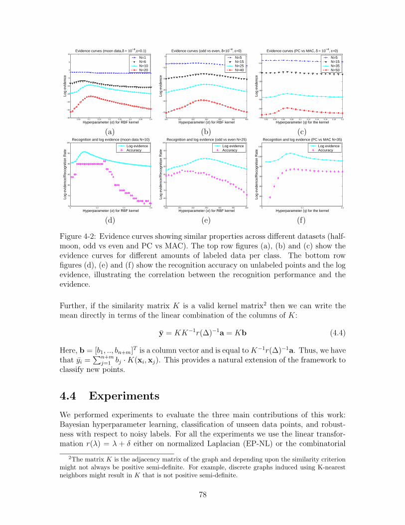
0.05 0.1 0.15 0.2 0.25 0.3 0.35 0.4−30

−25

−20

−15

−10

−5

0

5

10

Hyperparameter (σ) for RBF kernel

Log

evid

ence

Evidence curves (moon data,δ = 10−4,ε=0.1)

N=1N=6N=10N=20

100 150 200 250 300 350 400

−50

−40

−30

−20

−10

0

Hyperparameter (σ) for RBF kernel

Log

evid

ence

Evidence curves (odd vs even, δ=10−4, ε=0)

N=5N=15N=25N=40

0.02 0.04 0.06 0.08 0.1 0.12 0.14 0.16 0.18 0.2−70

−60

−50

−40

−30

−20

−10

0

Hyperparameter (γ) for the kernel

Log

evid

ence

Evidence curves (PC vs MAC, δ = 10−4, ε=0)

N=5N=15N=35N=50

(a) (b) (c)

0 0.2 0.4 0.670

75

80

85

90

95

100

Hyperparameter (σ) for RBF kernel

Log

evid

ence

/Rec

ogni

tion

Rat

e

Recognition and log evidence (moon data N=10)

Log evidenceAccuracy

100 150 200 250 300 350 40060

65

70

75

80

85

90

95

100

Hyperparameter (σ) for RBF kernel

Log

evid

ence

/Rec

ogni

tion

Rat

e

Recognition and log evidence (odd vs even N=25)

Log evidenceAccuracy

0 0.1 0.275

80

85

90

95

100

105

Hyperparameter (γ) for the kernel

Log

evid

ence

/Rec

ogni

tion

Rat

e

Recognition and log evidence (PC vs MAC N=35)

Log evidenceAccuracy

(d) (e) (f)

Figure 4-2: Evidence curves showing similar properties across different datasets (half-moon, odd vs even and PC vs MAC). The top row figures (a), (b) and (c) show theevidence curves for different amounts of labeled data per class. The bottom rowfigures (d), (e) and (f) show the recognition accuracy on unlabeled points and the logevidence, illustrating the correlation between the recognition performance and theevidence.

Further, if the similarity matrix K is a valid kernel matrix2 then we can write themean directly in terms of the linear combination of the columns of K:

y = KK−1r(∆)−1a = Kb (4.4)

Here, b = [b1, .., bn+m]T is a column vector and is equal toK−1r(∆)−1a. Thus, we havethat yi =

∑n+mj=1 bj ·K(xi,xj). This provides a natural extension of the framework to

classify new points.

4.4 Experiments

We performed experiments to evaluate the three main contributions of this work:Bayesian hyperparameter learning, classification of unseen data points, and robust-ness with respect to noisy labels. For all the experiments we use the linear transfor-mation r(λ) = λ + δ either on normalized Laplacian (EP-NL) or the combinatorial

2The matrix K is the adjacency matrix of the graph and depending upon the similarity criterionmight not always be positive semi-definite. For example, discrete graphs induced using K-nearestneighbors might result in K that is not positive semi-definite.

78

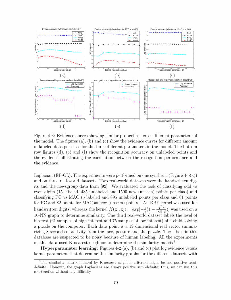
0 0.1 0.2 0.3 0.4 0.5−60

−50

−40

−30

−20

−10

0

Noise parameter (ε)

Log

evid

ence

Evidence curves (affect data, K=3, δ=10−4)

N=5N=15N=25N=40

1 2 3 4 5 6 7 8 9 10−50

−45

−40

−35

−30

−25

−20

−15

−10

−5

K in K−nearest neigbors

Log

evid

ence

Evidence curves (affect data, δ = 10−4, ε = 0.05)

N=5N=15N=25N=40

0 0.02 0.04 0.06 0.08 0.1 0.12−45

−40

−35

−30

−25

−20

−15

−10

−5

Transformation parameter (δ)

Log

evid

ence

Evidence curves (affect data, K = 3, ε = 0.05)

N=5N=15N=25N=40

(a) (b) (c)

0 0.05 0.1 0.15 0.2 0.25 0.3 0.35 0.4 0.45 0.560

65

70

75

80

85

90

95

100

Noise parameter (ε)

Log

evid

ence

/Rec

ogni

tion

Rat

e

Recognition and log evidence (affect data N=25)

Log evidenceAccuracy

1 2 3 4 5 6 7 8 9 10

60

65

70

75

80

85

90

95

100

K in K−nearest neigbors

Log

evid

ence

/Rec

ogni

tion

Rat

e

Recognition and log evidence (affect data N=25)

Log evidenceAccuracy

0 0.05 0.182

83

84

85

86

87

88

89

90

91

92

Transformation parameter (δ)

Log

evid

ence

/Rec

ogni

tion

Rat

e

Recognition and log evidence (affect data N=25)

Log evidenceAccuracy

(d) (e) (f)

Figure 4-3: Evidence curves showing similar properties across different parameters ofthe model. The figures (a), (b) and (c) show the evidence curves for different amountof labeled data per class for the three different parameters in the model. The bottomrow figures (d), (e) and (f) show the recognition accuracy on unlabeled points andthe evidence, illustrating the correlation between the recognition performance andthe evidence.

Laplacian (EP-CL). The experiments were performed on one synthetic (Figure 4-5(a))and on three real-world datasets. Two real-world datasets were the handwritten dig-its and the newsgroup data from [92]. We evaluated the task of classifying odd vseven digits (15 labeled, 485 unlabeled and 1500 new (unseen) points per class) andclassifying PC vs MAC (5 labeled and 895 unlabeled points per class and 61 pointsfor PC and 82 points for MAC as new (unseen) points). An RBF kernel was used for

handwritten digits, whereas the kernel K(xi,xj) = exp[− 1γ(1 −

xiT xj

|xi||xj|)] was used on a

10-NN graph to determine similarity. The third real-world dataset labels the level ofinterest (61 samples of high interest and 75 samples of low interest) of a child solvinga puzzle on the computer. Each data point is a 19 dimensional real vector summa-rizing 8 seconds of activity from the face, posture and the puzzle. The labels in thisdatabase are suspected to be noisy because of human labeling. All the experimentson this data used K-nearest neighbor to determine the similarity matrix3.

Hyperparameter learning: Figures 4-2 (a), (b) and (c) plot log evidence versuskernel parameters that determine the similarity graphs for the different datasets with

3The similarity matrix induced by K-nearest neighbor criterion might be not positive semi-definite. However, the graph Laplacians are always positive semi-definite; thus, we can use thisconstruction without any difficulty

79

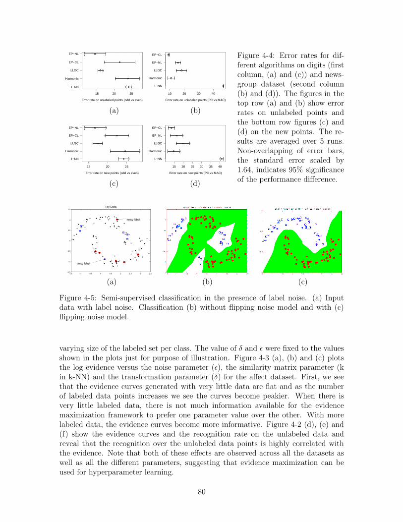
1−NN

Harmonic

LLGC

EP−CL

EP−NL

15 20 25

Error rate on unlabeled points (odd vs even)

1−NN

Harmonic

LLGC

EP−NL

EP−CL

10 20 30 40

Error rate on unlabeled points (PC vs MAC)

(a) (b)

1−NN

Harmonic

LLGC

EP−CL

EP−NL

15 20 25

Error rate on new points (odd vs even)

1−NN

Harmonic

LLGC

EP_NL

EP−CL

15 20 25 30 35 40

Error rate on new points (PC vs MAC)

(c) (d)

Figure 4-4: Error rates for dif-ferent algorithms on digits (firstcolumn, (a) and (c)) and news-group dataset (second column(b) and (d)). The figures in thetop row (a) and (b) show errorrates on unlabeled points andthe bottom row figures (c) and(d) on the new points. The re-sults are averaged over 5 runs.Non-overlapping of error bars,the standard error scaled by1.64, indicates 95% significanceof the performance difference.

−1.5 −1 −0.5 0 0.5 1 1.5 2 2.5−1.5

−1

−0.5

0

0.5

1

1.5Toy Data

noisy label

noisy label

(a) (b) (c)

Figure 4-5: Semi-supervised classification in the presence of label noise. (a) Inputdata with label noise. Classification (b) without flipping noise model and with (c)flipping noise model.

varying size of the labeled set per class. The value of δ and ε were fixed to the valuesshown in the plots just for purpose of illustration. Figure 4-3 (a), (b) and (c) plotsthe log evidence versus the noise parameter (ε), the similarity matrix parameter (kin k-NN) and the transformation parameter (δ) for the affect dataset. First, we seethat the evidence curves generated with very little data are flat and as the numberof labeled data points increases we see the curves become peakier. When there isvery little labeled data, there is not much information available for the evidencemaximization framework to prefer one parameter value over the other. With morelabeled data, the evidence curves become more informative. Figure 4-2 (d), (e) and(f) show the evidence curves and the recognition rate on the unlabeled data andreveal that the recognition over the unlabeled data points is highly correlated withthe evidence. Note that both of these effects are observed across all the datasets aswell as all the different parameters, suggesting that evidence maximization can beused for hyperparameter learning.

80

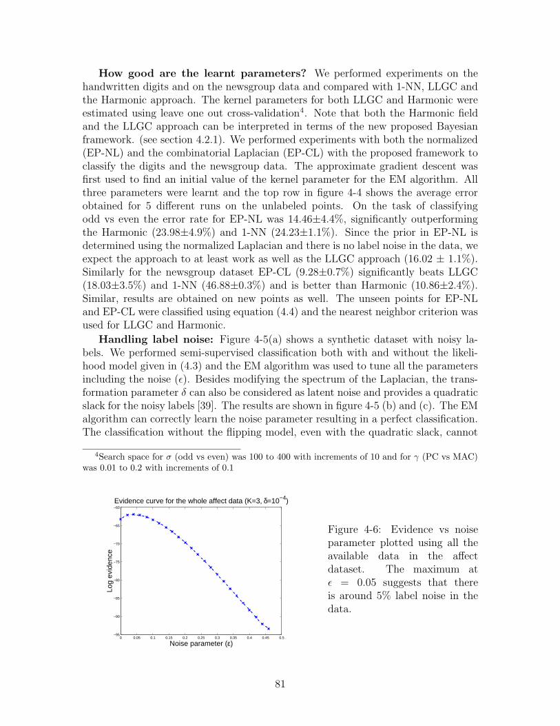
How good are the learnt parameters? We performed experiments on thehandwritten digits and on the newsgroup data and compared with 1-NN, LLGC andthe Harmonic approach. The kernel parameters for both LLGC and Harmonic wereestimated using leave one out cross-validation4. Note that both the Harmonic fieldand the LLGC approach can be interpreted in terms of the new proposed Bayesianframework. (see section 4.2.1). We performed experiments with both the normalized(EP-NL) and the combinatorial Laplacian (EP-CL) with the proposed framework toclassify the digits and the newsgroup data. The approximate gradient descent wasfirst used to find an initial value of the kernel parameter for the EM algorithm. Allthree parameters were learnt and the top row in figure 4-4 shows the average errorobtained for 5 different runs on the unlabeled points. On the task of classifyingodd vs even the error rate for EP-NL was 14.46±4.4%, significantly outperformingthe Harmonic (23.98±4.9%) and 1-NN (24.23±1.1%). Since the prior in EP-NL isdetermined using the normalized Laplacian and there is no label noise in the data, weexpect the approach to at least work as well as the LLGC approach (16.02 ± 1.1%).Similarly for the newsgroup dataset EP-CL (9.28±0.7%) significantly beats LLGC(18.03±3.5%) and 1-NN (46.88±0.3%) and is better than Harmonic (10.86±2.4%).Similar, results are obtained on new points as well. The unseen points for EP-NLand EP-CL were classified using equation (4.4) and the nearest neighbor criterion wasused for LLGC and Harmonic.

Handling label noise: Figure 4-5(a) shows a synthetic dataset with noisy la-bels. We performed semi-supervised classification both with and without the likeli-hood model given in (4.3) and the EM algorithm was used to tune all the parametersincluding the noise (ε). Besides modifying the spectrum of the Laplacian, the trans-formation parameter δ can also be considered as latent noise and provides a quadraticslack for the noisy labels [39]. The results are shown in figure 4-5 (b) and (c). The EMalgorithm can correctly learn the noise parameter resulting in a perfect classification.The classification without the flipping model, even with the quadratic slack, cannot

4Search space for σ (odd vs even) was 100 to 400 with increments of 10 and for γ (PC vs MAC)was 0.01 to 0.2 with increments of 0.1

0 0.05 0.1 0.15 0.2 0.25 0.3 0.35 0.4 0.45 0.5−95

−90

−85

−80

−75

−70

−65

−60

Noise parameter (ε)

Log

evid

ence

Evidence curve for the whole affect data (K=3, δ=10−4)

Figure 4-6: Evidence vs noiseparameter plotted using all theavailable data in the affectdataset. The maximum atε = 0.05 suggests that thereis around 5% label noise in thedata.

81

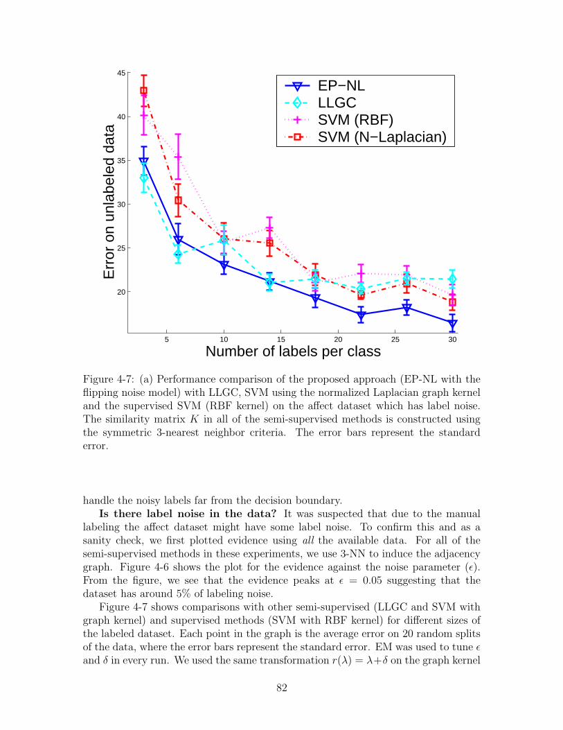
5 10 15 20 25 30

20

25

30

35

40

45

Number of labels per class

Err

or o

n un

labe

led

data

EP−NLLLGCSVM (RBF)SVM (N−Laplacian)

Figure 4-7: (a) Performance comparison of the proposed approach (EP-NL with theflipping noise model) with LLGC, SVM using the normalized Laplacian graph kerneland the supervised SVM (RBF kernel) on the affect dataset which has label noise.The similarity matrix K in all of the semi-supervised methods is constructed usingthe symmetric 3-nearest neighbor criteria. The error bars represent the standarderror.

handle the noisy labels far from the decision boundary.Is there label noise in the data? It was suspected that due to the manual

labeling the affect dataset might have some label noise. To confirm this and as asanity check, we first plotted evidence using all the available data. For all of thesemi-supervised methods in these experiments, we use 3-NN to induce the adjacencygraph. Figure 4-6 shows the plot for the evidence against the noise parameter (ε).From the figure, we see that the evidence peaks at ε = 0.05 suggesting that thedataset has around 5% of labeling noise.

Figure 4-7 shows comparisons with other semi-supervised (LLGC and SVM withgraph kernel) and supervised methods (SVM with RBF kernel) for different sizes ofthe labeled dataset. Each point in the graph is the average error on 20 random splitsof the data, where the error bars represent the standard error. EM was used to tune εand δ in every run. We used the same transformation r(λ) = λ+δ on the graph kernel

82

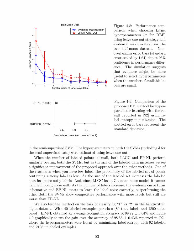
2 3 4 5 6 7 8 9 100

5

10

15

20

Total number of labels available

Err

or o

n un

labe

led

data

Half Moon Data

Evidence MaximizationLeave−One−Out

Figure 4-8: Performance com-parison when choosing kernelhyperparameters (σ for RBF)using leave-one-out strategy andevidence maximization on thetwo half-moon dataset. Non-overlapping error bars (standarderror scaled by 1.64) depict 95%confidence in performance differ-ence. The simulation suggeststhat evidence might be moreuseful to select hyperparameterswhen the number of available la-bels are small.

Harmonic (N = 92)

EP−NL (N = 80)

0.5 1.0 1.5

Error rate on unlabeled points (1 vs 2)

Figure 4-9: Comparison of theproposed EM method for hyper-parameter learning with the re-sult reported in [92] using la-bel entropy minimization. Theplotted error bars represent thestandard deviation.

in the semi-supervised SVM. The hyperparameters in both the SVMs (including δ forthe semi-supervised case) were estimated using leave one out.

When the number of labeled points is small, both LLGC and EP-NL performsimilarly beating both the SVMs, but as the size of the labeled data increases we seea significant improvement of the proposed approach over the other methods. One ofthe reasons is when you have few labels the probability of the labeled set of pointscontaining a noisy label is low. As the size of the labeled set increases the labeleddata has more noisy labels. And, since LLGC has a Gaussian noise model, it cannothandle flipping noise well. As the number of labels increase, the evidence curve turnsinformative and EP-NL starts to learn the label noise correctly, outperforming theother Both the SVMs show competitive performance with more labels but still areworse than EP-NL.

We also test the method on the task of classifying “1” vs “2” in the handwrittendigits dataset. With 40 labeled examples per class (80 total labels and 1800 unla-beled), EP-NL obtained an average recognition accuracy of 99.72 ± 0.04% and figure4-9 graphically shows the gain over the accuracy of 98.56 ± 0.43% reported in [92],where the hyperparameters were learnt by minimizing label entropy with 92 labeledand 2108 unlabeled examples.

83

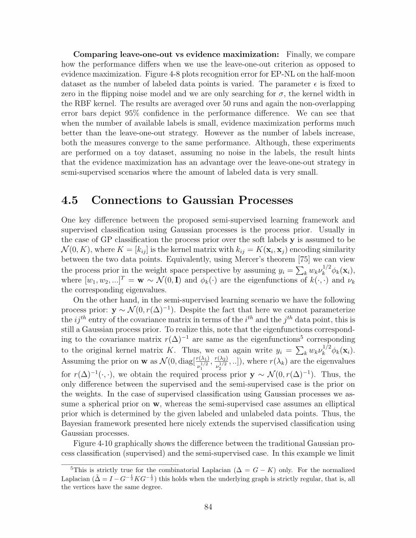
Comparing leave-one-out vs evidence maximization: Finally, we comparehow the performance differs when we use the leave-one-out criterion as opposed toevidence maximization. Figure 4-8 plots recognition error for EP-NL on the half-moondataset as the number of labeled data points is varied. The parameter ε is fixed tozero in the flipping noise model and we are only searching for σ, the kernel width inthe RBF kernel. The results are averaged over 50 runs and again the non-overlappingerror bars depict 95% confidence in the performance difference. We can see thatwhen the number of available labels is small, evidence maximization performs muchbetter than the leave-one-out strategy. However as the number of labels increase,both the measures converge to the same performance. Although, these experimentsare performed on a toy dataset, assuming no noise in the labels, the result hintsthat the evidence maximization has an advantage over the leave-one-out strategy insemi-supervised scenarios where the amount of labeled data is very small.

4.5 Connections to Gaussian Processes

One key difference between the proposed semi-supervised learning framework andsupervised classification using Gaussian processes is the process prior. Usually inthe case of GP classification the process prior over the soft labels y is assumed to beN (0, K), whereK = [kij] is the kernel matrix with kij = K(xi,xj) encoding similaritybetween the two data points. Equivalently, using Mercer’s theorem [75] we can view

the process prior in the weight space perspective by assuming yi =∑

k wkν1/2k φk(xi),

where [w1, w2, ...]T = w ∼ N (0, I) and φk(·) are the eigenfunctions of k(·, ·) and νk

the corresponding eigenvalues.On the other hand, in the semi-supervised learning scenario we have the following

process prior: y ∼ N (0, r(∆)−1). Despite the fact that here we cannot parameterizethe ijth entry of the covariance matrix in terms of the ith and the jth data point, this isstill a Gaussian process prior. To realize this, note that the eigenfunctions correspond-ing to the covariance matrix r(∆)−1 are same as the eigenfunctions5 corresponding

to the original kernel matrix K. Thus, we can again write yi =∑

k wkν1/2k φk(xi).

Assuming the prior on w as N (0, diag[ r(λ1)

ν1/21

, r(λ2)

ν1/22

, ..]), where r(λk) are the eigenvalues

for r(∆)−1(·, ·), we obtain the required process prior y ∼ N (0, r(∆)−1). Thus, theonly difference between the supervised and the semi-supervised case is the prior onthe weights. In the case of supervised classification using Gaussian processes we as-sume a spherical prior on w, whereas the semi-supervised case assumes an ellipticalprior which is determined by the given labeled and unlabeled data points. Thus, theBayesian framework presented here nicely extends the supervised classification usingGaussian processes.

Figure 4-10 graphically shows the difference between the traditional Gaussian pro-cess classification (supervised) and the semi-supervised case. In this example we limit

5This is strictly true for the combinatorial Laplacian (∆ = G − K) only. For the normalized

Laplacian (∆ = I −G−

12 KG−

12 ) this holds when the underlying graph is strictly regular, that is, all

the vertices have the same degree.

84

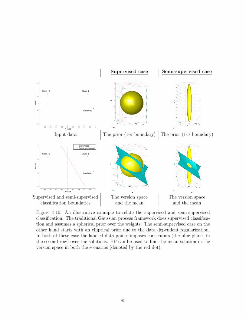
Supervised case Semi-supervised case

−0.8 −0.6 −0.4 −0.2 0 0.2 0.4 0.6 0.8 1

−1.5

−1

−0.5

0

0.5

1

1.5

Class 1Class −1

Unlabeled

X−axis

Y−

axis

Input data The prior (1-σ boundary) The prior (1-σ boundary)

−0.8 −0.6 −0.4 −0.2 0 0.2 0.4 0.6 0.8 1

−1.5

−1

−0.5

0

0.5

1

1.5

Class 1Class −1

Unlabeled

X−axis

Y−

axis

SupervisedSemi−supervised

Supervised and semi-supervised The version space The version spaceclassification boundaries and the mean and the mean

Figure 4-10: An illustrative example to relate the supervised and semi-supervisedclassification. The traditional Gaussian process framework does supervised classifica-tion and assumes a spherical prior over the weights. The semi-supervised case on theother hand starts with an elliptical prior due to the data dependent regularization.In both of these case the labeled data points imposes constraints (the blue planes inthe second row) over the solutions. EP can be used to find the mean solution in theversion space in both the scenarios (denoted by the red dot).

85

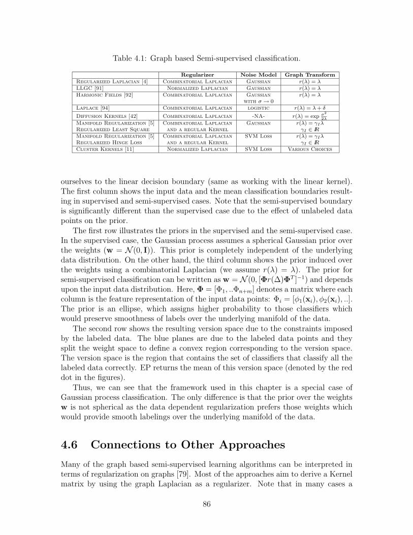
Table 4.1: Graph based Semi-supervised classification.

Regularizer Noise Model Graph Transform

Regularized Laplacian [4] Combinatorial Laplacian Gaussian r(λ) = λLLGC [91] Normalized Laplacian Gaussian r(λ) = λHarmonic Fields [92] Combinatorial Laplacian Gaussian r(λ) = λ

with σ → 0Laplace [94] Combinatorial Laplacian logistic r(λ) = λ + δ

Diffusion Kernels [42] Combinatorial Laplacian -NA- r(λ) = exp σ2

2λManifold Regularization [5] Combinatorial Laplacian Gaussian r(λ) = γIλRegularized Least Square and a regular Kernel γI ∈ IRManifold Regularization [5] Combinatorial Laplacian SVM Loss r(λ) = γIλRegularized Hinge Loss and a regular Kernel γI ∈ IRCluster Kernels [11] Normalized Laplacian SVM Loss Various Choices

ourselves to the linear decision boundary (same as working with the linear kernel).The first column shows the input data and the mean classification boundaries result-ing in supervised and semi-supervised cases. Note that the semi-supervised boundaryis significantly different than the supervised case due to the effect of unlabeled datapoints on the prior.

The first row illustrates the priors in the supervised and the semi-supervised case.In the supervised case, the Gaussian process assumes a spherical Gaussian prior overthe weights (w = N (0, I)). This prior is completely independent of the underlyingdata distribution. On the other hand, the third column shows the prior induced overthe weights using a combinatorial Laplacian (we assume r(λ) = λ). The prior forsemi-supervised classification can be written as w = N (0, [Φr(∆)ΦT ]−1) and dependsupon the input data distribution. Here, Φ = [Φ1, ..Φn+m] denotes a matrix where eachcolumn is the feature representation of the input data points: Φi = [φ1(xi), φ2(xi), ..].The prior is an ellipse, which assigns higher probability to those classifiers whichwould preserve smoothness of labels over the underlying manifold of the data.

The second row shows the resulting version space due to the constraints imposedby the labeled data. The blue planes are due to the labeled data points and theysplit the weight space to define a convex region corresponding to the version space.The version space is the region that contains the set of classifiers that classify all thelabeled data correctly. EP returns the mean of this version space (denoted by the reddot in the figures).

Thus, we can see that the framework used in this chapter is a special case ofGaussian process classification. The only difference is that the prior over the weightsw is not spherical as the data dependent regularization prefers those weights whichwould provide smooth labelings over the underlying manifold of the data.

4.6 Connections to Other Approaches

Many of the graph based semi-supervised learning algorithms can be interpreted interms of regularization on graphs [79]. Most of the approaches aim to derive a Kernelmatrix by using the graph Laplacian as a regularizer. Note that in many cases a

86

monotonic function might be applied to modify the spectrum of the graph Laplacianbefore using it as a regularizer. For different choices of Laplacian (Combinatorialor Normalized) and different choices of the transformation function, we can derivethe regularizers for most of the graph based semi-supervised learning approaches.Moreover, there is a duality between the Kernels in Reproducing Kernel Hilbert Spaceand the Gaussian process priors which allows us to translate the regularizers in termsof prior probabilities. Thus, we can induce process priors, which are Gaussian, forsemi-supervised learning motivated by the regularization on graphs.

Many of the graph based semi-supervised learning techniques were derived inde-pendently; thus, there are other differences besides just the process prior. One suchdifference is the noise model or the likelihood. Even though, some of the work has justfocused on deriving the graph kernels [11, 42, 79], where these kernels can be used inan SVM classification formulation, there have been approaches where different noisemodels have been used. For example, Gaussian noise has been frequently used [91]and it has the advantage that the solutions can be often obtained as closed form ex-pressions. Similarly, Zhu et al [94] have used a noise model based on logistic function,which is perhaps a more natural noise model than the Gaussian one. However, thereis no closed form solution when using this noise model and an approximation (forexample Laplace or EP) is warranted. The null category noise model [48] is anothernoise model that has been introduced for semi-supervised classification. We wouldlike to point out that much of the semi-supervised learning work has focused on thesmoothness constraints over the graph without paying much attention to the noisemodel. That is, most of the work so far has been focused on exploiting the informa-tion from the unlabeled points without really caring about different kinds of noisethe training data might have. We feel that modeling noise is a very important aspectand a complete semi-supervised learning framework should focus both on the processprior and the noise model as well. The Bayesian framework described here aims tocover both of these aspects and provides us insight to many of these semi-supervisedlearning methods.

Table 4.1 summarizes many of the recent graph based semi-supervised learningmethods and their interpretation in terms of the Bayesian framework. By choosingdifferent kinds of Laplacians, different noise models and a different transformation ofthe graph spectrum, we can derive all of these methods. Most of the graph basedmethods aim to provide a solution that respect the labels in the training data but alsoconsider an appropriate regularization term that depends upon the underlying graph.The Bayesian interpretation stems from the fact that the regularizers can be usedto induce a prior over the possible labelings and together with the likelihood termsthat favor the solution consistent with the training data, we can tie most of thesemethods in a single framework. Note that there is no easy Bayesian interpretation ofSVM loss. There have been attempts in the past and perhaps the null category noisemodel introduced by Lawrence and Jordan [48] is the closest. Nonetheless, by viewingall of these methods in the Bayesian perspective, we can exploit techniques such asevidence maximization to choose hyperparameters for these methods. Further, givena new dataset we now have a tool for choosing the best performing algorithms betweenthese graph based methods.

87

Also, note that even though the transductive SVMs [86] and the semi-supervisedclassification using the null category noise model [48] are not graph based methods,they can still be subsumed under this Bayesian perspective. Lawrence and Jordanhave used null category noise model together with the Gaussian process prior; hence,besides the Gaussian process prior the only difference between their method and graphbased techniques is the noise model. Further, the proposed null category noise modelimitates the SVM hinge loss for classification. Thus, taking into account the dualitybetween regularization in RKHS and the Gaussian process prior, we can relate thetransductive SVM and the Gaussian process formulation.

4.7 Conclusion and Future Work

We have presented and evaluated a new method for learning hyperparameters forgraph-based semi-supervised classification in a Bayesian framework. The results in-dicate that evidence maximization works well for learning hyperparameters, includingthe amount of label noise in the data.

Computational complexity: The computational complexity for the evidencemaximization procedure is O(n3), where n is the number of data points, due to matrixinversion required to compute the gradient.

Convergence issues: Since the proposed algorithm is based on gradient descentand EM, it suffers from some of the disadvantages of these algorithms. The EMalgorithm is guaranteed to converge at a local optimum; consequently, the algorithmmay not always provide the best solution. One possible way to alleviate this problem isto provide good initializations to the parameters using any available prior knowledge.Further, we can do a very coarse search over the parameter space to find good initialestimates.

Possible improvements: A very interesting direction would be to incorporatekernel alignment measures to reduce the search space as well as to obtain good initialestimates for the parameters and the hyper parameters. Further, sparsification on thelines of [17] would help a lot to reduce the computational complexity of the evidencemaximization procedure.

88

Chapter 5

Located Hidden Random Fields toLearn Discriminative Parts

This chapter1 introduces the Located Hidden Random Field (LHRF), a conditionalmodel for simultaneous part-based detection and segmentation of events or objects ofa given class. Given some training data with coarse labels, the LHRF automaticallylearns a set of parts (the finer labels) that are both discriminative and informativeabout the relative position (either spatial or temporal) with respect to the coarselabels provided for training.

Parts based object detection and segmentation from images is one task where thesemodels can be used very effectively. The idea in the discriminative framework is totrain a network of classifiers that can first detect parts of objects and then combinethere inferences to segment out the complete object from the image. However, it isvery difficult and tedious to obtain training images labeled for each individual part.Thus, we need a model that can reliably learn parts from segmentation masks only(which are considered coarse labels). LHRF solves this problem by introducing a set oflatent variables, which correspond to parts and are hidden during the training phase.By introducing the global position of the object as a latent variable, the LHRF modelsthe long-range spatial configuration of these parts, as well as their local interactions.Experiments on benchmark datasets show that the use of discriminative parts leads tostate-of-the-art detection and segmentation performance, with the additional benefitof obtaining a labeling of the object’s component parts.

Although most of the discussion in this chapter focuses around the problem ofobject detection and segmentation from the images, we would like to point out thatthe proposed model can be very easily applied to activity recognition and affectrecognition scenarios.

1All of the work described from section 5.2 to section 5.6 was done in collaboration with JohnWinn during the summer internship in 2005 at Microsoft Research, Cambridge, UK. This work isunder review for European Conference on Computer Vision, 2006.

89

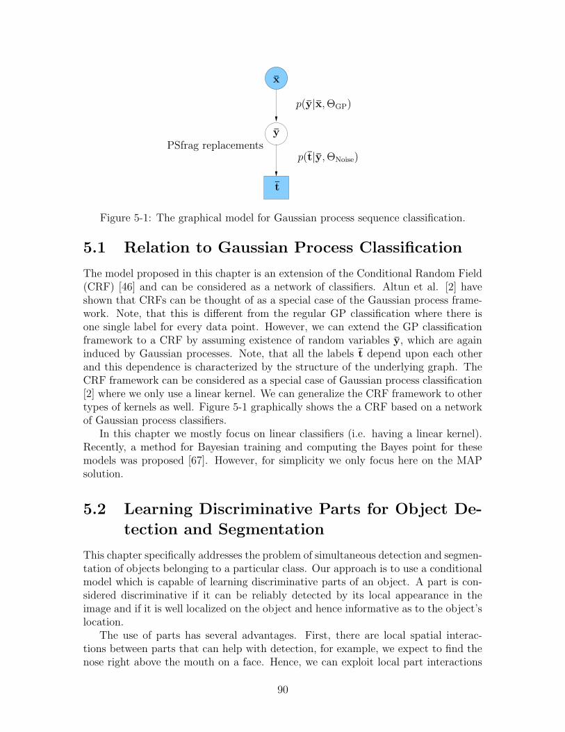
PSfrag replacementsy

x

t

p(y|x,ΘGP)

p(t|y,ΘNoise)

Figure 5-1: The graphical model for Gaussian process sequence classification.

5.1 Relation to Gaussian Process Classification

The model proposed in this chapter is an extension of the Conditional Random Field(CRF) [46] and can be considered as a network of classifiers. Altun et al. [2] haveshown that CRFs can be thought of as a special case of the Gaussian process frame-work. Note, that this is different from the regular GP classification where there isone single label for every data point. However, we can extend the GP classificationframework to a CRF by assuming existence of random variables y, which are againinduced by Gaussian processes. Note, that all the labels t depend upon each otherand this dependence is characterized by the structure of the underlying graph. TheCRF framework can be considered as a special case of Gaussian process classification[2] where we only use a linear kernel. We can generalize the CRF framework to othertypes of kernels as well. Figure 5-1 graphically shows the a CRF based on a networkof Gaussian process classifiers.

In this chapter we mostly focus on linear classifiers (i.e. having a linear kernel).Recently, a method for Bayesian training and computing the Bayes point for thesemodels was proposed [67]. However, for simplicity we only focus here on the MAPsolution.

5.2 Learning Discriminative Parts for Object De-

tection and Segmentation

This chapter specifically addresses the problem of simultaneous detection and segmen-tation of objects belonging to a particular class. Our approach is to use a conditionalmodel which is capable of learning discriminative parts of an object. A part is con-sidered discriminative if it can be reliably detected by its local appearance in theimage and if it is well localized on the object and hence informative as to the object’slocation.

The use of parts has several advantages. First, there are local spatial interac-tions between parts that can help with detection, for example, we expect to find thenose right above the mouth on a face. Hence, we can exploit local part interactions

90

to exclude invalid hypotheses at a local level. Second, knowing the location of onepart highly constrains the locations of other parts. For example, knowing the lo-cations of wheels of a car constrains the positions where the rest of the car can bedetected. Thus, we can improve object detection by incorporating long range spatialconstraints on the parts. Third, by inferring a part labeling for the training data,we can accurately assess the variability in the appearance of each part, giving betterpart detection and hence better object detection. Finally, the use of parts gives thepotential for detecting objects even if they are partially occluded.

One possibility for training a parts-based system is to use supervised training withhand-labeled parts. The disadvantage of this approach is that it is very expensive toget training data annotated for parts, plus it is unclear which parts should be selected.Existing generative approaches try to address these problems by clustering visuallysimilar image patches to build a codebook in the hope that clusters correspond todifferent parts of the object. However, this codebook has to allow for all sources ofvariability in appearance. We provide a discriminative alternative where irrelevantsources of variability do not need to be modeled.

This chapter introduces Located Hidden Random Field, a novel extension to theConditional Random Field [46] that can learn parts discriminatively. We introduce alatent part label for each pixel which is learned simultaneously with model parameters,given the segmentation mask for the object. Further, the object’s position is explicitlyrepresented in the model, allowing long-range spatial interactions between differentobject parts to be learned.

5.3 Related Work

There have been a number of parts-based approaches to segmentation or detection.It is possible to pre-select which parts are used as in Crandall et al. [16] – however,this requires significant human effort for each new object class. Alternatively, partscan be learned by clustering visually similar image patches [1, 49] but this approachdoes not exploit the spatial layout of the parts in the training images. There has beenwork with generative models that do learn spatially coherent parts in an unsupervisedmanner. For example, the constellation models of Fergus et al. [21] learn parts whichoccur in a particular spatial arrangement. However, the parts correspond to sparselydetected interest points and so parts are limited in size, cannot represent untexturedregions and do not provide a segmentation of the image. More recently, Winn andJojic [90] used a dense generative model to learn a partitioning of the object intoparts, along with an unsupervised segmentation of the object. Their method doesnot learn a model of object appearance (only of object shape) and so cannot be usedfor object detection in cluttered images.

As well as unsupervised methods, there are a range of supervised methods for seg-mentation and detection. Ullman and Borenstein [8] use a fragment-based method forsegmentation, but do not provide detection results. Shotton et al. [77] use a boostingmethod based on image contours for detection, but this does not lead to a segmen-tation. There are a number of methods using Conditional Random Fields (CRFs) to

91

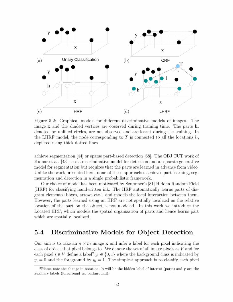
(a) Unary Classification

y

x

(b) CRF

y

x

(c) HRF

y

h

x

(d)

h

x

y

T

l

LHRF

Figure 5-2: Graphical models for different discriminative models of images. Theimage x and the shaded vertices are observed during training time. The parts h,denoted by unfilled circles, are not observed and are learnt during the training. Inthe LHRF model, the node corresponding to T is connected to all the locations li,depicted using thick dotted lines.

achieve segmentation [44] or sparse part-based detection [68]. The OBJ CUT work ofKumar et al. [43] uses a discriminative model for detection and a separate generativemodel for segmentation but requires that the parts are learned in advance from video.Unlike the work presented here, none of these approaches achieves part-learning, seg-mentation and detection in a single probabilistic framework.

Our choice of model has been motivated by Szummer’s [81] Hidden Random Field(HRF) for classifying handwritten ink. The HRF automatically learns parts of dia-gram elements (boxes, arrows etc.) and models the local interaction between them.However, the parts learned using an HRF are not spatially localized as the relativelocation of the part on the object is not modeled. In this work we introduce theLocated HRF, which models the spatial organization of parts and hence learns partwhich are spatially localized.

5.4 Discriminative Models for Object Detection

Our aim is to take an n ×m image x and infer a label for each pixel indicating theclass of object that pixel belongs to. We denote the set of all image pixels as V and foreach pixel i ∈ V define a label2 yi ∈ {0, 1} where the background class is indicated byyi = 0 and the foreground by yi = 1. The simplest approach is to classify each pixel

2Please note the change in notation. h will be the hidden label of interest (parts) and y are theauxiliary labels (foreground vs. background).

92

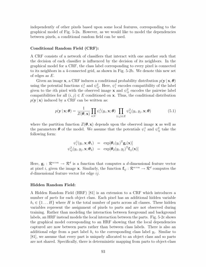
independently of other pixels based upon some local features, corresponding to thegraphical model of Fig. 5-2a. However, as we would like to model the dependenciesbetween pixels, a conditional random field can be used.

Conditional Random Field (CRF):

A CRF consists of a network of classifiers that interact with one another such thatthe decision of each classifier is influenced by the decision of its neighbors. In thegraphical model for a CRF, the class label corresponding to every pixel is connectedto its neighbors in a 4-connected grid, as shown in Fig. 5-2b. We denote this new setof edges as E.

Given an image x, a CRF induces a conditional probability distribution p(y |x,θ)using the potential functions ψ1

i and ψ2ij. Here, ψ1

i encodes compatibility of the labelgiven to the ith pixel with the observed image x and ψ2

ij encodes the pairwise labelcompatibilities for all (i, j) ∈ E conditioned on x. Thus, the conditional distributionp(y |x) induced by a CRF can be written as:

p(y |x; θ) =1

Z(θ,x)

∏

i∈V

ψ1i (yi,x; θ)

∏

(i,j)∈E

ψ2ij(yi, yj,x; θ) (5.1)

where the partition function Z(θ,x) depends upon the observed image x as well asthe parameters θ of the model. We assume that the potentials ψ1

i and ψ2ij take the

following form:

ψ1i (yi,x; θ1) = exp[θ1(yi)

Tgi(x)]

ψ2ij(yi, yj,x; θ2) = exp[θ2(yi, yj)

Tfij(x)]

Here, gi : Rn×m → Rd is a function that computes a d-dimensional feature vectorat pixel i, given the image x. Similarly, the function fij : Rn×m → Rd computes thed-dimensional feature vector for edge ij.

Hidden Random Field:

A Hidden Random Field (HRF) [81] is an extension to a CRF which introduces anumber of parts for each object class. Each pixel has an additional hidden variablehi ∈ {1 . . . H} where H is the total number of parts across all classes. These hiddenvariables represent the assignment of pixels to parts and are not observed duringtraining. Rather than modeling the interaction between foreground and backgroundlabels, an HRF instead models the local interaction between the parts. Fig. 5-2c showsthe graphical model corresponding to an HRF showing that the local dependenciescaptured are now between parts rather than between class labels. There is also anadditional edge from a part label hi to the corresponding class label yi. Similar to[81], we assume that every part is uniquely allocated to an object class and so partsare not shared. Specifically, there is deterministic mapping from parts to object-class

93

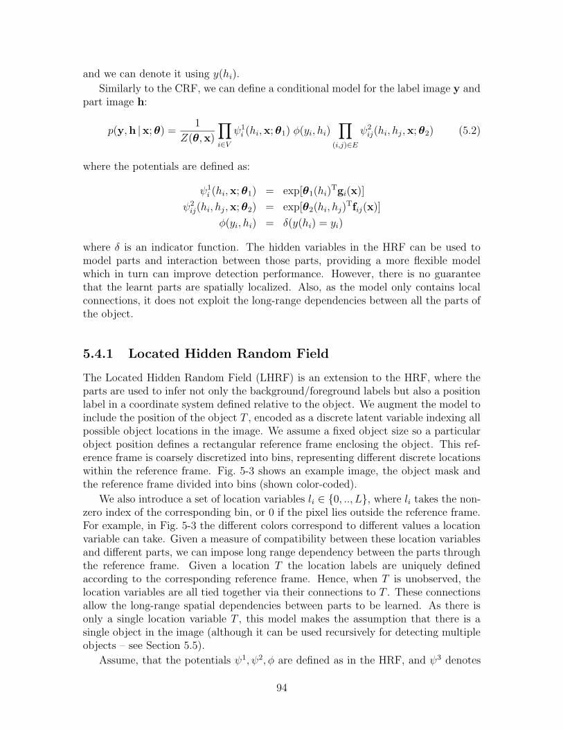
and we can denote it using y(hi).

Similarly to the CRF, we can define a conditional model for the label image y andpart image h:

p(y,h |x; θ) =1

Z(θ,x)

∏

i∈V

ψ1i (hi,x; θ1) φ(yi, hi)

∏

(i,j)∈E

ψ2ij(hi, hj,x; θ2) (5.2)

where the potentials are defined as:

ψ1i (hi,x; θ1) = exp[θ1(hi)

Tgi(x)]

ψ2ij(hi, hj,x; θ2) = exp[θ2(hi, hj)

Tfij(x)]

φ(yi, hi) = δ(y(hi) = yi)

where δ is an indicator function. The hidden variables in the HRF can be used tomodel parts and interaction between those parts, providing a more flexible modelwhich in turn can improve detection performance. However, there is no guaranteethat the learnt parts are spatially localized. Also, as the model only contains localconnections, it does not exploit the long-range dependencies between all the parts ofthe object.

5.4.1 Located Hidden Random Field

The Located Hidden Random Field (LHRF) is an extension to the HRF, where theparts are used to infer not only the background/foreground labels but also a positionlabel in a coordinate system defined relative to the object. We augment the model toinclude the position of the object T , encoded as a discrete latent variable indexing allpossible object locations in the image. We assume a fixed object size so a particularobject position defines a rectangular reference frame enclosing the object. This ref-erence frame is coarsely discretized into bins, representing different discrete locationswithin the reference frame. Fig. 5-3 shows an example image, the object mask andthe reference frame divided into bins (shown color-coded).

We also introduce a set of location variables li ∈ {0, .., L}, where li takes the non-zero index of the corresponding bin, or 0 if the pixel lies outside the reference frame.For example, in Fig. 5-3 the different colors correspond to different values a locationvariable can take. Given a measure of compatibility between these location variablesand different parts, we can impose long range dependency between the parts throughthe reference frame. Given a location T the location labels are uniquely definedaccording to the corresponding reference frame. Hence, when T is unobserved, thelocation variables are all tied together via their connections to T . These connectionsallow the long-range spatial dependencies between parts to be learned. As there isonly a single location variable T , this model makes the assumption that there is asingle object in the image (although it can be used recursively for detecting multipleobjects – see Section 5.5).

Assume, that the potentials ψ1, ψ2, φ are defined as in the HRF, and ψ3 denotes

94

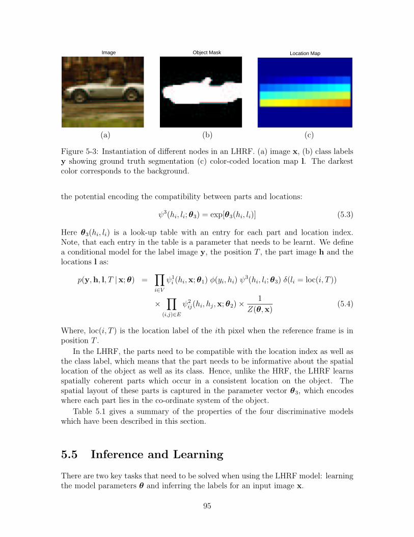
Image Object Mask Location Map

(a) (b) (c)

Figure 5-3: Instantiation of different nodes in an LHRF. (a) image x, (b) class labelsy showing ground truth segmentation (c) color-coded location map l. The darkestcolor corresponds to the background.

the potential encoding the compatibility between parts and locations:

ψ3(hi, li; θ3) = exp[θ3(hi, li)] (5.3)

Here θ3(hi, li) is a look-up table with an entry for each part and location index.Note, that each entry in the table is a parameter that needs to be learnt. We definea conditional model for the label image y, the position T , the part image h and thelocations l as:

p(y,h, l, T |x; θ) =∏

i∈V

ψ1i (hi,x; θ1) φ(yi, hi) ψ

3(hi, li; θ3) δ(li = loc(i, T ))

×∏

(i,j)∈E

ψ2ij(hi, hj,x; θ2) ×

1

Z(θ,x)(5.4)

Where, loc(i, T ) is the location label of the ith pixel when the reference frame is inposition T .

In the LHRF, the parts need to be compatible with the location index as well asthe class label, which means that the part needs to be informative about the spatiallocation of the object as well as its class. Hence, unlike the HRF, the LHRF learnsspatially coherent parts which occur in a consistent location on the object. Thespatial layout of these parts is captured in the parameter vector θ3, which encodeswhere each part lies in the co-ordinate system of the object.

Table 5.1 gives a summary of the properties of the four discriminative modelswhich have been described in this section.

5.5 Inference and Learning

There are two key tasks that need to be solved when using the LHRF model: learningthe model parameters θ and inferring the labels for an input image x.

95

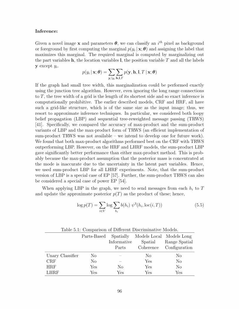
Inference:

Given a novel image x and parameters θ, we can classify an ith pixel as backgroundor foreground by first computing the marginal p(yi |x; θ) and assigning the label thatmaximizes this marginal. The required marginal is computed by marginalizing outthe part variables h, the location variables l, the position variable T and all the labelsy except yi.

p(yi |x; θ) =∑

y/yi

∑

h,l,T

p(y,h, l, T |x; θ)

If the graph had small tree width, this marginalization could be performed exactlyusing the junction tree algorithm. However, even ignoring the long range connectionsto T , the tree width of a grid is the length of its shortest side and so exact inference iscomputationally prohibitive. The earlier described models, CRF and HRF, all havesuch a grid-like structure, which is of the same size as the input image; thus, weresort to approximate inference techniques. In particular, we considered both loopybelief propagation (LBP) and sequential tree-reweighted message passing (TRWS)[41]. Specifically, we compared the accuracy of max-product and the sum-productvariants of LBP and the max-product form of TRWS (an efficient implementation ofsum-product TRWS was not available – we intend to develop one for future work).We found that both max-product algorithms performed best on the CRF with TRWSoutperforming LBP. However, on the HRF and LHRF models, the sum-product LBPgave significantly better performance than either max-product method. This is prob-ably because the max-product assumption that the posterior mass is concentrated atthe mode is inaccurate due to the uncertainty in the latent part variables. Hence,we used sum-product LBP for all LHRF experiments. Note, that the sum-productversion of LBP is a special case of EP [57]. Further, the sum-product TRWS can alsobe considered a special case of power EP [54].

When applying LBP in the graph, we need to send messages from each hi to Tand update the approximate posterior p(T ) as the product of these; hence,

log p(T ) =∑

i∈V

log∑

hi

b(hi) ψ3(hi, loc(i, T )) (5.5)

Table 5.1: Comparison of Different Discriminative Models.

Parts-Based Spatially Models Local Models LongInformative Spatial Range Spatial

Parts Coherence Configuration

Unary Classifier No – No NoCRF No – Yes NoHRF Yes No Yes NoLHRF Yes Yes Yes Yes

96

where b(hi) is the product of messages into the ith node, excluding the message fromT . To speed up the computation of p(T ), we make the following approximation:

log p(T ) ≈∑

i∈V

∑

hi

b(hi) logψ3(hi, loc(i, T )). (5.6)

This posterior can now be computed very efficiently using convolutions.

Parameter Learning:

Given an image x with labels y and location map l, the parameters θ are learnt bymaximizing the conditional likelihood p(y, l|x,θ) multiplied by the Gaussian priorp(θ) = N (θ|0, σ2I). Hence, we seek to maximize the objective function F(θ) =L(θ) + log p(θ), where L(θ) is the log of the conditional likelihood.

F(θ) = log p(y, l|x; θ) + log p(θ) = log∑

h

p(y,h, l|x; θ) + log p(θ)

= − logZ(θ,x) + log∑

h

p(y,h, l,x; θ) + log p(θ) (5.7)

where:

p(y,h, l,x; θ) =∏

i

ψ1i (hi,x; θ1)φ(yi, hi)ψ

3(hi, li; θ3)∏

(i,j)∈E

ψ2ij(hi, hj,x; θ2).

We use gradient ascent to maximize the objective with respect to the parametersθ. The derivative of the log likelihood L(θ) with respect to the model parametersθ = {θ1,θ2,θ3} can be written in terms of the features, single node marginals andpairwise marginals:

δL(θ)

δθ1(h′)=

∑

i∈V

gi(x) · (p(hi =h′|x,y, l; θ) − p(hi =h

′|x; θ))

δL(θ)

δθ2(h′, h′′)=

∑

(i,j)∈E

fij(x) · (p(hi =h′, hj =h′′|x,y, l; θ) − p(hi =h

′, hj =h′′|x; θ))

δL(θ)

δθ3(h′, l′)=

∑

i∈V

p(hi =h′, li = l

′|x,y, l; θ) − p(hi =h′, li = l

′|x; θ)

It is intractable to compute the partition function Z(θ,x) and hence the objectivefunction (5.7) cannot be computed exactly. Instead, we use the approximation to thepartition function given by the LBP or TRWS inference algorithm, which is also usedto provide approximations to the marginals required to compute the derivative of theobjective. Notice that the location variable T comes into effect only when computingmarginals for the unclamped model (where y and l are not observed), as the sum over

97

l should be restricted to those configurations consistent with a value of T . We havetrained the model both with and without this restriction. Better detection resultsare achieved without it. This is for two reasons: including this restriction makes themodel very sensitive to changes in image size and secondly, when used for detectingmultiple objects, the restriction of a single object instance does not apply, and henceshould not be included when training part detectors.

Image Features:

We aim to use image features which are informative about the part label but invariantto changes in illumination and small changes in pose. The features used in this workfor both unary and pairwise potentials are Scale Invariant Feature Transform (SIFT)descriptors [50], except that we compute these descriptors at only one scale and donot rotate the descriptor, due to the assumption of fixed object scale and rotation.For efficiency of learning, we apply the model at a coarser resolution than the pixelresolution – the results given in this chapter use a grid whose nodes correspond to 2×2pixel squares. For the unary potentials, SIFT descriptors are computed at the centerof the each grid square. For the edge potentials, the SIFT descriptors are computed atthe location half-way between two neighboring squares. To allow parameter sharingbetween horizontal and vertical edge potentials, the features corresponding to thevertical edges in the graphs are rotated by 90 degrees. Note, that the compatibilitiesbetween the parts are captured using these SIFT features. Rotating the features by90 degrees for the vertical edges allows us to use the same set of parameters to encodethe compatibilities of parts in both the horizontal and vertical directions.

Detecting multiple objects:

Our model assumes that a single object is present in the image. We can rejectimages with no objects by comparing the evidence for this model with the evidencefor a background-only model. Specifically, for each given image we compute theapproximation of p(model |x,θ), which is the normalization constant Z(θ,x) in (5.4).This model evidence is compared with the evidence for a model which labels the entireimage as background p(noobject |x,θ). By defining a prior on these two models, wedefine the threshold on the ratio of the model evidences used to determine if an objectis present or absent. By varying this prior, we can obtain precision-recall curves fordetection.

We can use this methodology to detect multiple objects in a single image, byapplying the model recursively. Given an image, we detect whether it contains anobject instance. If we detect an object, the unary potentials are set to uniform forall pixels labeled as foreground. The model is then reapplied to detect further objectinstances. This process is repeated until no further objects are detected.

98

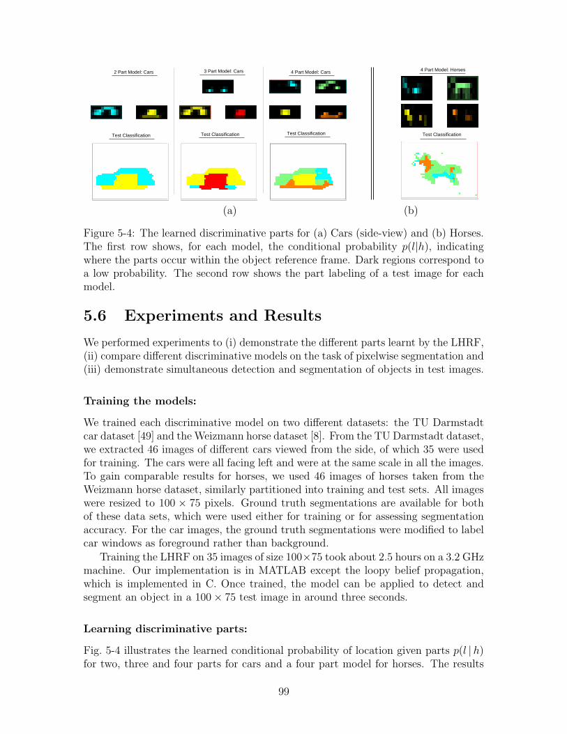
Test Classification Test Classification Test Classification

4 Part Model: Cars2 Part Model: Cars 3 Part Model: Cars

Test Classification

4 Part Model: Horses

(a) (b)

Figure 5-4: The learned discriminative parts for (a) Cars (side-view) and (b) Horses.The first row shows, for each model, the conditional probability p(l|h), indicatingwhere the parts occur within the object reference frame. Dark regions correspond toa low probability. The second row shows the part labeling of a test image for eachmodel.

5.6 Experiments and Results

We performed experiments to (i) demonstrate the different parts learnt by the LHRF,(ii) compare different discriminative models on the task of pixelwise segmentation and(iii) demonstrate simultaneous detection and segmentation of objects in test images.

Training the models:

We trained each discriminative model on two different datasets: the TU Darmstadtcar dataset [49] and the Weizmann horse dataset [8]. From the TU Darmstadt dataset,we extracted 46 images of different cars viewed from the side, of which 35 were usedfor training. The cars were all facing left and were at the same scale in all the images.To gain comparable results for horses, we used 46 images of horses taken from theWeizmann horse dataset, similarly partitioned into training and test sets. All imageswere resized to 100 × 75 pixels. Ground truth segmentations are available for bothof these data sets, which were used either for training or for assessing segmentationaccuracy. For the car images, the ground truth segmentations were modified to labelcar windows as foreground rather than background.

Training the LHRF on 35 images of size 100×75 took about 2.5 hours on a 3.2 GHzmachine. Our implementation is in MATLAB except the loopy belief propagation,which is implemented in C. Once trained, the model can be applied to detect andsegment an object in a 100 × 75 test image in around three seconds.

Learning discriminative parts:

Fig. 5-4 illustrates the learned conditional probability of location given parts p(l |h)for two, three and four parts for cars and a four part model for horses. The results

99

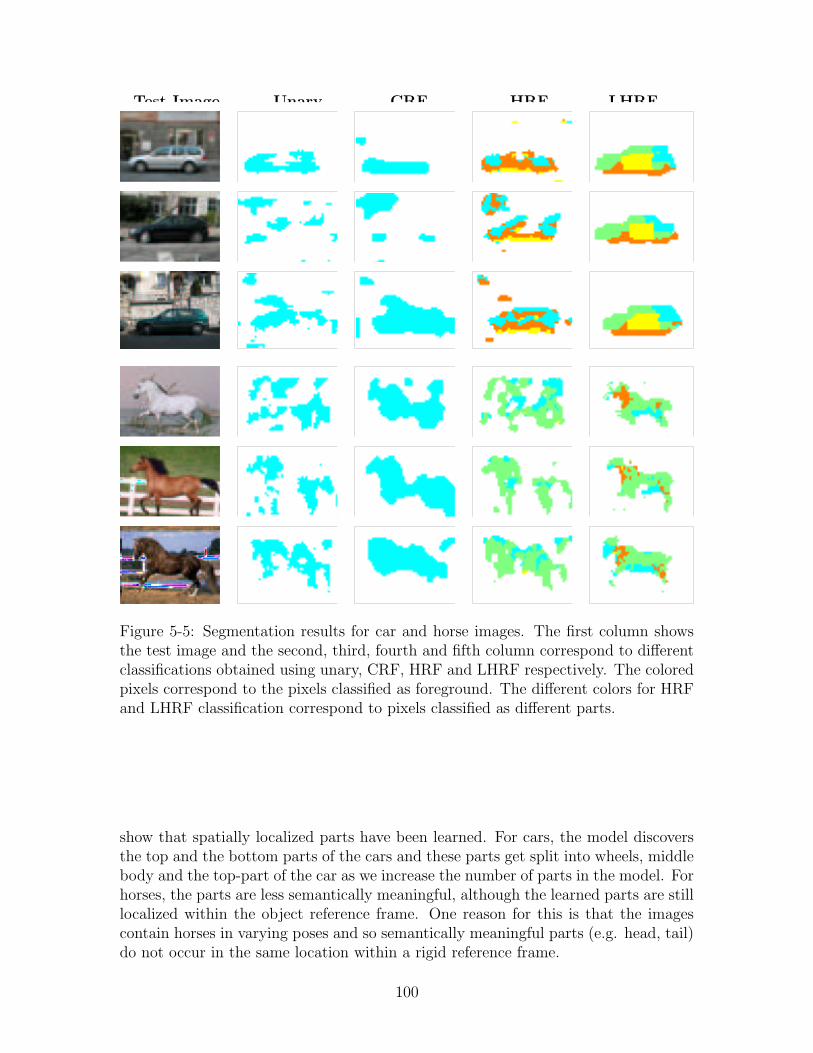
Test Image Unary CRF HRF LHRF

Figure 5-5: Segmentation results for car and horse images. The first column showsthe test image and the second, third, fourth and fifth column correspond to differentclassifications obtained using unary, CRF, HRF and LHRF respectively. The coloredpixels correspond to the pixels classified as foreground. The different colors for HRFand LHRF classification correspond to pixels classified as different parts.

show that spatially localized parts have been learned. For cars, the model discoversthe top and the bottom parts of the cars and these parts get split into wheels, middlebody and the top-part of the car as we increase the number of parts in the model. Forhorses, the parts are less semantically meaningful, although the learned parts are stilllocalized within the object reference frame. One reason for this is that the imagescontain horses in varying poses and so semantically meaningful parts (e.g. head, tail)do not occur in the same location within a rigid reference frame.

100

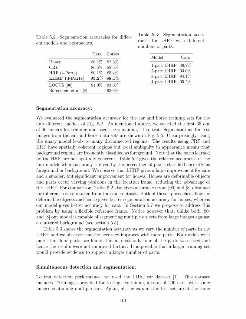
Table 5.2: Segmentation accuracies for differ-ent models and approaches.

Cars Horses

Unary 86.1% 82.3%CRF 86.5% 83.6%HRF (4-Parts) 90.1% 85.4%LHRF (4-Parts) 95.2% 88.1%

LOCUS [90] 94.0% 93.0%Borenstein et al. [8] - 93.6%

Table 5.3: Segmentation accu-racies for LHRF with differentnumbers of parts.

Model Cars

1-part LHRF 89.7%2-part LHRF 93.0%3-part LHRF 94.1%4-part LHRF 95.2%

Segmentation accuracy:

We evaluated the segmentation accuracy for the car and horse training sets for thefour different models of Fig. 5-2. As mentioned above, we selected the first 35 outof 46 images for training and used the remaining 11 to test. Segmentations for testimages from the car and horse data sets are shown in Fig. 5-5. Unsurprisingly, usingthe unary model leads to many disconnected regions. The results using CRF andHRF have spatially coherent regions but local ambiguity in appearance means thatbackground regions are frequently classified as foreground. Note that the parts learnedby the HRF are not spatially coherent. Table 5.2 gives the relative accuracies of thefour models where accuracy is given by the percentage of pixels classified correctly asforeground or background. We observe that LHRF gives a large improvement for carsand a smaller, but significant improvement for horses. Horses are deformable objectsand parts occur varying positions in the location frame, reducing the advantage ofthe LHRF. For comparison, Table 5.2 also gives accuracies from [90] and [8] obtainedfor different test sets taken from the same dataset. Both of these approaches allow fordeformable objects and hence gives better segmentation accuracy for horses, whereasour model gives better accuracy for cars. In Section 5.7 we propose to address thisproblem by using a flexible reference frame. Notice however that, unlike both [90]and [8] our model is capable of segmenting multiple objects from large images againsta cluttered background (see section 5.5).

Table 5.3 shows the segmentation accuracy as we vary the number of parts in theLHRF and we observe that the accuracy improves with more parts. For models withmore than four parts, we found that at most only four of the parts were used andhence the results were not improved further. It is possible that a larger training setwould provide evidence to support a larger number of parts.

Simultaneous detection and segmentation:

To test detection performance, we used the UIUC car dataset [1]. This datasetincludes 170 images provided for testing, containing a total of 200 cars, with someimages containing multiple cars. Again, all the cars in this test set are at the same

101

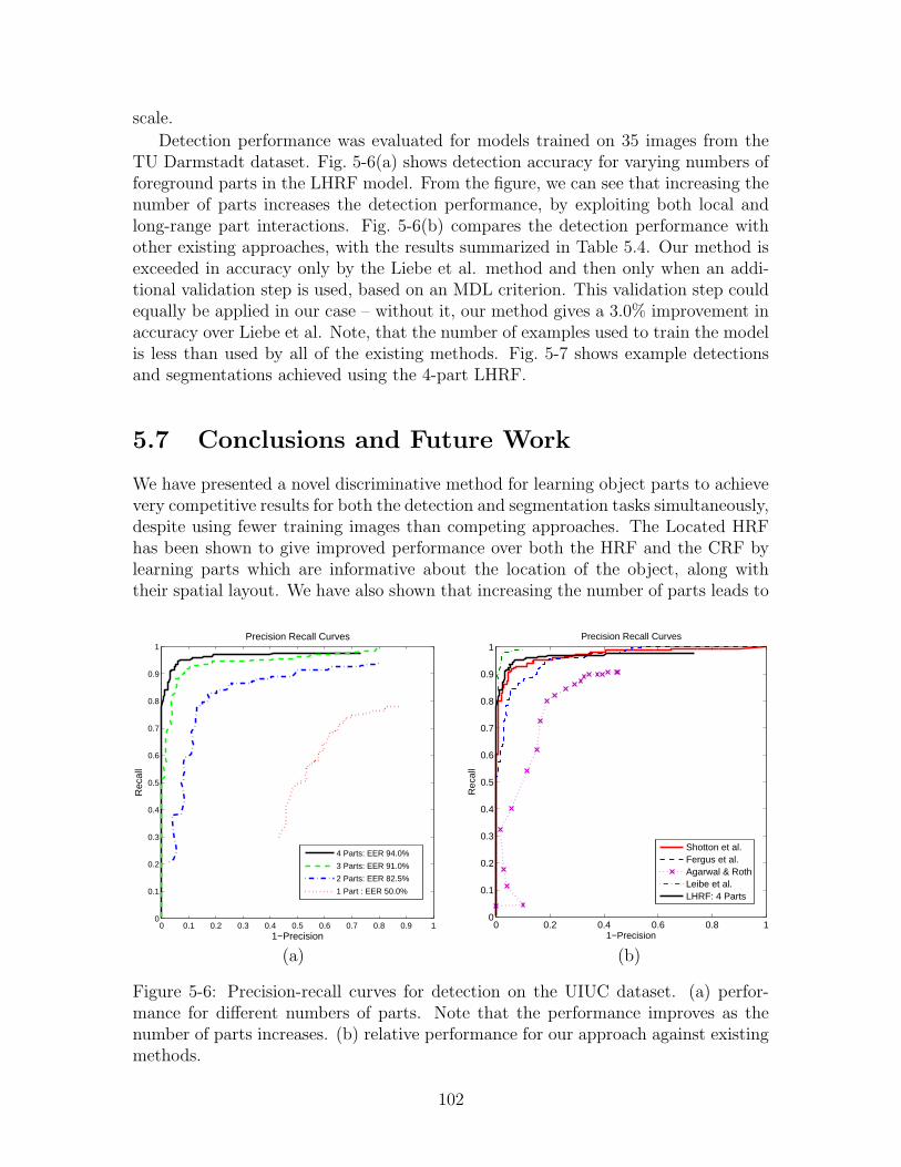
scale.

Detection performance was evaluated for models trained on 35 images from theTU Darmstadt dataset. Fig. 5-6(a) shows detection accuracy for varying numbers offoreground parts in the LHRF model. From the figure, we can see that increasing thenumber of parts increases the detection performance, by exploiting both local andlong-range part interactions. Fig. 5-6(b) compares the detection performance withother existing approaches, with the results summarized in Table 5.4. Our method isexceeded in accuracy only by the Liebe et al. method and then only when an addi-tional validation step is used, based on an MDL criterion. This validation step couldequally be applied in our case – without it, our method gives a 3.0% improvement inaccuracy over Liebe et al. Note, that the number of examples used to train the modelis less than used by all of the existing methods. Fig. 5-7 shows example detectionsand segmentations achieved using the 4-part LHRF.

5.7 Conclusions and Future Work

We have presented a novel discriminative method for learning object parts to achievevery competitive results for both the detection and segmentation tasks simultaneously,despite using fewer training images than competing approaches. The Located HRFhas been shown to give improved performance over both the HRF and the CRF bylearning parts which are informative about the location of the object, along withtheir spatial layout. We have also shown that increasing the number of parts leads to

0 0.1 0.2 0.3 0.4 0.5 0.6 0.7 0.8 0.9 10

0.1

0.2

0.3

0.4

0.5

0.6

0.7

0.8

0.9

1

1−Precision

Rec

all

Precision Recall Curves

4 Parts: EER 94.0%

3 Parts: EER 91.0%

2 Parts: EER 82.5%

1 Part : EER 50.0%

0 0.2 0.4 0.6 0.8 10

0.1

0.2

0.3

0.4

0.5

0.6

0.7

0.8

0.9

1

1−Precision

Rec

all

Precision Recall Curves

Shotton et al.Fergus et al.Agarwal & RothLeibe et al.LHRF: 4 Parts

(a) (b)

Figure 5-6: Precision-recall curves for detection on the UIUC dataset. (a) perfor-mance for different numbers of parts. Note that the performance improves as thenumber of parts increases. (b) relative performance for our approach against existingmethods.

102

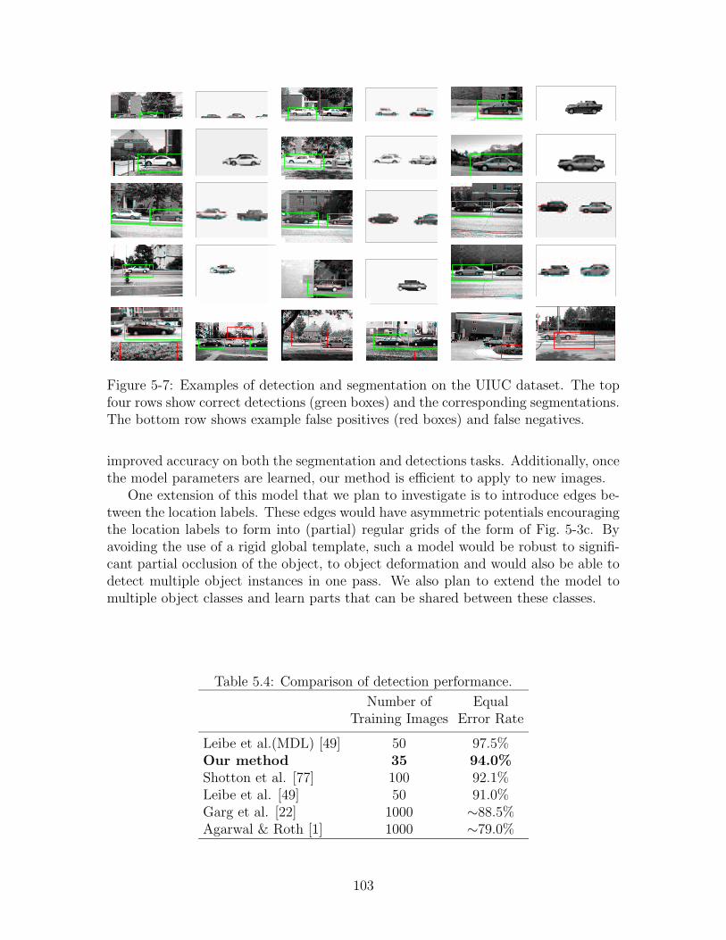
Figure 5-7: Examples of detection and segmentation on the UIUC dataset. The topfour rows show correct detections (green boxes) and the corresponding segmentations.The bottom row shows example false positives (red boxes) and false negatives.

improved accuracy on both the segmentation and detections tasks. Additionally, oncethe model parameters are learned, our method is efficient to apply to new images.

One extension of this model that we plan to investigate is to introduce edges be-tween the location labels. These edges would have asymmetric potentials encouragingthe location labels to form into (partial) regular grids of the form of Fig. 5-3c. Byavoiding the use of a rigid global template, such a model would be robust to signifi-cant partial occlusion of the object, to object deformation and would also be able todetect multiple object instances in one pass. We also plan to extend the model tomultiple object classes and learn parts that can be shared between these classes.

Table 5.4: Comparison of detection performance.

Number of EqualTraining Images Error Rate

Leibe et al.(MDL) [49] 50 97.5%Our method 35 94.0%Shotton et al. [77] 100 92.1%Leibe et al. [49] 50 91.0%Garg et al. [22] 1000 ∼88.5%Agarwal & Roth [1] 1000 ∼79.0%

103

104

Chapter 6

Conclusion and Future Work

6.1 Summary

In this thesis we proposed various extensions to learn discriminative models withdifferent types of incomplete data. Specifically, the proposed techniques handle fourdifferent kinds of incompleteness arising due to incorrect labels, incomplete features,partially labeled data and data annotated with coarse labels. The framework pro-vides insights and connections to many existing methods in semi-supervised learning,sensor-fusion and discriminative modeling and one major advantage of viewing differ-ent methods in a single Bayesian framework is that we can use evidence maximizationto perform model selection tasks, which were non-trivial earlier. Also, we can nowexploit the modularity of the unified framework to combine different aspects of in-completeness and derive new methods for discriminative modeling.

In the following, we highlight the major contributions of the work:

• Noisy Labels: Section 2.1.2 discusses different noise models that can be usedto handle different kinds of noise in the label. In section 2.4 Gaussian pro-cess classification is applied to the challenging problem of detecting quittersin a learning environment and we highlight kernel learning via the EM-EP al-gorithm. We also demonstrate on different datasets that the right choice ofnoise model can provide significant gains. We highlight scenarios in human-computer interaction and computer vision, where the incorrect labels might notlie near the decision boundary, thus, cannot be modeled using the linear or thequadratic slack. For these scenarios, we empirically show that the flipping noisemodel outperforms other slack based noise models. One of the advantages ofthis Bayesian framework is that we can use evidence maximization criteria toselect the noise model and its parameters.

• Incomplete Features: The incompleteness due to missing features is handledby combining the decisions of experts trained on subsets of features, where thedecision fusion ignores the classifiers that act on the missing features. In section3.2, we proposed a unified approach using a mixture of Gaussian Processes forachieving sensor fusion under the challenging conditions of missing channels.

105

We provide an algorithm for Bayesian inference designed with a fast update ofclassification decisions based on variational and Gaussian approximations. Insection 3.3.2 we demonstrate experiments on the task of classifying affectivestate of interest using multimodal information with missing data. The mixtureof GP method outperformed feature level fusion based on imputation and sev-eral standard classifier combination schemes and obtained a recognition rate ofover 86%. The experiments also show that there are significant gains when theincomplete data is incorporated in the training set. Finally, we demonstrate amultimodal affect recognition system capable of tracking facial features, pos-tures and classifying affective states of children in a learning environment.

• Partially Labeled Data: We present extensions of Gaussian Process classifi-cation using data dependent regularization. The resulting framework connectsmany recent graph based semi-supervised learning efforts [79, 91, 92, 94]. In-ference in the models with the non-Gaussian likelihoods are carried out usingExpectation Propagation, which provides better approximations than the pre-viously used Laplace approximation [94], with an additional benefit of derivingan EM-algorithm that exploits evidence maximization to learn the kernel andthe hyperparameters of the model. Additionally using the same machinery, theframework can explicitly model and estimate the different types of label noisein the data. The experiments in section 4.4 show that the evidence maximiza-tion can be effectively exploited to learn hyperparameters of the model. Onthe half-moon dataset we demonstrate experimentally that when the number ofavailable labeled data points are small the hyperparameter selection using ev-idence maximization should be preferred over the leave-one-out strategy. Fur-ther, as demonstrated on the affect dataset, we can conclude that modelinglabel noise appropriately in the model leads to significant gains. Finally, manydifferent Graph-based approaches can be viewed in the Bayesian perspective,consequently suggesting that evidence maximization can be utilized to tune thehyperparameters of those methods as well.

• Coarse Labels: In section 5.4.1 the located hidden random field (LHRF) wasintroduced, which extends the traditional discriminative frameworks like condi-tional random fields and the hidden random random fields. These models havebeen shown to be specially effective on computer vision tasks and we use theproposed framework to address the problem of part-based object detection andrecognition. Experiments in section 5.6 shows how LHRF learns object parts toachieve very competitive results for both the detection and segmentation taskssimultaneously, despite using fewer training images than competing approaches.The Located HRF has been shown to give improved performance over both theHRF and the CRF by learning parts which are informative about the locationof the object, along with their spatial layout. We have also shown that increas-ing the number of parts leads to improved accuracy on both the segmentationand detection tasks. Additionally, once the model parameters are learned, ourmethod is efficient to apply to new images.

106

6.2 Application Scenarios

The highly challenging problems addressed in this work are motivated by problemsin affective computing, activity recognition and machine perception. Specifically, theproposed framework in the thesis can be used in any scenario that needs analysisand machine learning from data that arises from multiple channels, having very fewlabels and annotations, some of which might be incorrect or coarsely annotated.There are several research application scenarios that encounter incompleteness dueto multimodal data, or the challenge of annotating the enormous amount of corpuswith the labels of interest. Below, we briefly describe some of the possible applicationswhere the techniques proposed in this thesis can be applied:

• Affective Computing: Pattern recognition for affective computing can veryeffectively use some of the methods described in this thesis. Besides, handlingmultimodal data, this thesis provides a rigorous framework to handle uncer-tainty and resolution of the labels which often plagues affect recognition prob-lems. A lot of the methods described in this thesis can significantly reducethe pre-processing time by exploiting semi-supervised classification and also byallowing incorrectly labeled examples. Further, there is always a question ofright set of emotions to detect in an affective computing scenario. The locatedhidden random field offers a solution where the exact emotions are discoveredautomatically based upon some coarser level categorization such as mood.

• Sensor Networks and Context Aware Applications: Sensor networks isan area where a lot of applications require fusion of information from multiplesources. Further, there might be other energy or environmental constraintsthat prohibit the sensors from sending complete observations. Then there areother applications that involve analyzing multi-sensory data collected throughcellular phones and PDAs to learn human and social networks. Often, thesescenarios result in a huge amount of data which can be very hard to annotateand semi-supervised learning and HRF based models can be applied to theseapplications as well.

• Man-Machine Interaction: The proposed framework can be an importantcomponent in a machine learning system that aims to interact naturally withpeople. Applications that need to learn to be adaptive to the users internalstate would find this system useful. Similarly, the robotic characters and virtualavatars can incorporate the proposed methods and algorithms to enhance theirperceptual capabilities. Note, that once trained the kernel classifiers for theaffect recognition tasks takes around a few milliseconds to classifiy a new point.One of the advantage of the discriminative models is that the classificationcan be performed quickly; thus, they can be easily used with the real-timecharacters.

• Computer Vision: There are many applications in computer vision besidesobject detection and segmentation. There are imminent application of semi-supervised learning in tracking objects in videos. The consecutive frames in the

107

videos often lie in a low-dimensional manifold; hence, they can exploit the infor-mation from other unannotated frames to recover variables of interest. Further,often it is tedious to obtain very good annotations or labels in the videos dueto insufficient resolution. The coarse and label noise models can be effectivelyused in those scenarios. Finally, Gaussian process regression, classification andtheir extensions can be applied to learn from examples effectively.

6.3 Future Work

There are many opportunities for future work relating to Gaussian process classifica-tion, their extensions and applications to real-world scenarios.

Gaussian process classification in general is more flexible than some of the otherdiscriminative counterparts. And as shown in this thesis it can be extended to handleproblem specific scenarios. However, to achieve a popularity equal to other methodssuch as SVMs, the computational time needs to be reduced. There have been sparseGP based classification methods [17, 47] and an interesting direction is to combinethese approaches with the extensions proposed in this thesis.

Further despite anecdotal evidence, the convergence of Expectation Propagationfor Gaussian process classification is not well understood theoretically. It can beshown that EP is an energy minimization procedure. However, the energy it minimizesis not necessarily convex. One interesting direction would be to convexify the EPobjective using techniques such as power EP. Besides guaranteed convergence convexEP might also be able to provide insights to the issue of convergence in regular EP.Further, we should also investigate semidefinite relaxations of the EP objective asthere are efficient methods to solve these problems and these can alleviate some ofthe computational challenges in Gaussian process classification.

Recently, there has been much interest in semi-supervised learning of the struc-tured data. As a lot of models that handle structured data are probabilistic, aninteresting question is how to extend the discriminative framework to handle thesecases. Can we combine the generative models such as Hidden Markov Models (HMMs)and the discriminative framework, such that they “co-train” each other?

Evidence maximization has been a method of choice for model selection tasks.However, evidence is not well-defined for the class of models with improper priors.An interesting question is how can we perform model selection in these cases? Arethere other metrics besides evidence maximization that we can use? Further, we needto compare different model selection criteria such as evidence maximization and leave-one-out cross-validation. Are there cases in which one measure should be preferredover others?

There are many extensions to the proposed LHRF model for the purpose of objectdetection. Currently, LHRF can handle rigid objects well, but might not perform wellwhen the objects are deformable. One possible extension of this model is to intro-duce edges between the location labels. Such a model would be robust to significantpartial occlusion of the object, to object deformation and would also be able todetect multiple object instances in one pass. Further, the LHRF can be extended

108

to model multiple object classes and learn parts that can be shared between theseclasses. Finally, we should also apply HRF and LHRF to activity recognition andother applications in human-computer interaction.

An exciting possibility is incorporation of active learning and other decision theo-retic formulations that consider cost-benefit trade offs in obtaining different kinds oflabels. Further, there are interesting possibilities where the mixture of GPs model iscombined with different noise models, semi-supervised classification and other exten-sions proposed in these thesis.

Finally, this thesis shows the discriminative models can be expressive enough tohandle different kinds of incompleteness. There are many applications in differentdomains such as sensor networks, social networks and other multimodal scenarioswhere the proposed method can be used effectively. Further depending upon theapplications, the kind of incompleteness encountered can be different then the oneshandled here, requiring us to develop other extensions which are theoretically andpractically interesting.

109

110

Appendix A

Feature Extraction for AffectRecognition

There are many different features we use for affect recognition in learning environ-ments. The non-verbal behaviors can be sensed through a camera, a pressure sensingchair, a pressure mouse and a device that measure the skin conductance. The camerais equipped with Infrared (IR) LEDs for structured lighting that help in real-timetracking of pupils and extracting other features from the face. Similarly the datasensed through the chair is used to extract information about the postures. Featuresare extracted from the activity that the subject is doing on the computer as well,which are then sent to a multimodal pattern analyzer that combines all the infor-mation to predict the current affective state. Below we describe the algorithms toextract features from these different sensors.

A.1 Facial Features & Head Gestures

The feature extraction module for face and head gestures is shown in figure A(a).We use an in-house built version of the IBM Blue Eyes Camera that tracks pupilsunobtrusively using two sets of IR LEDs. One set of LEDs is on the optical axis andproduces the red eye effect. The two sets of LEDs are switched on and off to generatetwo interlaced images for a single frame.The image where the on-axis LEDs are onhas white pupils whereas the image where the off-axis LEDs are on has black pupils.These two images are subtracted to get a difference image, which is used to track thepupils. The pupils are detected and tracked using the difference image, which is noisydue to the motion artifacts and other specularities. We have elsewhere described [34]an algorithm to track pupils reliably using the noisy difference image. Once tracked,the pupil positions are passed to an HMM based head-nod and head-shake detectionsystem,which provides the likelihoods of head-nods and head-shakes. Similarly, wehave also trained an HMM that uses the radii of the visible pupil as inputs to producethe likelihoods of blinks. Further, we use the system described in [34] to recover shapeinformation of eyes and the eyebrows.

Given pupil positions we can also localize the image around the mouth. Rather

111

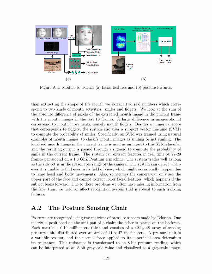
(a) (b)

Figure A-1: Module to extract (a) facial features and (b) posture features.

than extracting the shape of the mouth we extract two real numbers which corre-spond to two kinds of mouth activities: smiles and fidgets. We look at the sum ofthe absolute difference of pixels of the extracted mouth image in the current framewith the mouth images in the last 10 frames. A large difference in images shouldcorrespond to mouth movements, namely mouth fidgets. Besides a numerical scorethat corresponds to fidgets, the system also uses a support vector machine (SVM)to compute the probability of smiles. Specifically, an SVM was trained using naturalexamples of mouth images, to classify mouth images as smiling or not smiling. Thelocalized mouth image in the current frame is used as an input to this SVM classifierand the resulting output is passed through a sigmoid to compute the probability ofsmile in the current frame. The system can extract features in real time at 27-29frames per second on a 1.8 GhZ Pentium 4 machine. The system tracks well as longas the subject is in the reasonable range of the camera. The system can detect when-ever it is unable to find eyes in its field of view, which might occasionally happen dueto large head and body movements. Also, sometimes the camera can only see theupper part of the face and cannot extract lower facial features, which happens if thesubject leans forward. Due to these problems we often have missing information fromthe face; thus, we need an affect recognition system that is robust to such trackingfailures.

A.2 The Posture Sensing Chair

Postures are recognized using two matrices of pressure sensors made by Tekscan. Onematrix is positioned on the seat-pan of a chair; the other is placed on the backrest.Each matrix is 0.10 millimeters thick and consists of a 42-by-48 array of sensingpressure units distributed over an area of 41 x 47 centimeters. A pressure unit isa variable resistor, and the normal force applied to its superficial area determinesits resistance. This resistance is transformed to an 8-bit pressure reading, whichcan be interpreted as an 8-bit grayscale value and visualized as a grayscale image.

112

Figure A(b) shows the feature extraction strategy used for postures in [59]. First,the pressure maps sensed by the chair are pre-processed to remove noise and thestructure of the map is modeled with a mixture of Gaussians. The parameters of theGaussian mixture (means and variances) are used to feed a 3-layer feed-forward neuralnetwork that classifies the static set of postures (for example, sitting upright, leaningback, etc.) and activity level (low, medium and high) in real time at 8 frames persecond, which are then used as posture features by the multimodal affect classificationmodule.

A.3 Detecting Interest: Final Set of Features

This is the new section I added to describe the features used in affect recognition.Table A.1 shows the extracted features from the face, the posture and the game statethat were used for the task of recognizing the affective state of interest in learningenvironments (Chapter 3).

There are two features extracted from the game. They correspond to the state ofthe game and the level of difficulty. The state of the game indicates if a new gamehas started or ended, or whether the child asked for a hint, or whether the solutionprovided was correct etc. In this work, all the game features were manually extracted.

The posture recognition system can extract features at 8 frames per second (fps).The facial feature tracker performs at 27-29 frames per second, but we subsamplethe observations to 8 fps to extract the final features. Each sample in the databasesummarizes 8 seconds of activity. Specifically, we average the values of the features(see table A.1) observed continuously for 8 secs (64 frames). Note, that the samplesdo not explicitly encode any temporal dynamics of the feature over the 8 seconds ofactivity and only represent the average values.

The same database is used for experiments in Chapter 4, except that rather thanusing the automatically extracted features, we use manually coded action units basedon the Facial Action Coding System (FACS)[20]. Specifically, from the face trackerwe extract a 6 dimensional feature that encodes the average presence of an actionunit (AU 1,2, 4, 5, 6, 7).

113

Table A.1: Extracted features for the task of detecting interest.

Face Posture GameTracker Sensor Information

2D vector encoding 1D vector encoding 1D vector encodingstandard deviation in average activity level average difficulty level

(x, y) positions of pupilsin the frame

Average likelihood of shakes 5D vector encoding 6D vector encodingAverage likelihood of nods average number of frames average number of framesAverage likelihood of blink in postures: in the game state:

Average probability of fidget {leaning forward, sitting upright, {new game, game running

leaning backward, slumped back, success, failure

Average probability of smile sitting on edge} hint error, hint help}

4D vector encodingthe shape of the eyes

and the brows

114

Bibliography

[1] S. Agarwal and D. Roth. Learning a sparse representation for object detection.In European Conference on Computer Vision, 2002.

[2] Y. Altun, T. Hofmann, and A. Smola. Gaussian process classification for seg-menting and annotating sequences. In International Conference on Machine

Learning, 2004.

[3] M. J. Beal. Variational Algorithms for Approximate Bayesian Inference. PhDthesis, University College London, 2003.

[4] M. Belkin and P. Niyogi. Semi-supervised learning on riemannian manifolds.Machine Learning, Special Issue on Clustering, 56, 2004.

[5] M. Belkin, P. Niyogi, and V. Sindhwani. On manifold regularization. In Work-

shop on AI and Statistics, 2005.

[6] A. Blum and S. Chawla. Learning with labeled and unlabeled data using graphmincuts. In ICML, 2001.

[7] A. Blum and T. Mitchell. Combining labeled and unlabeled data with co-training. In Proceedings of the Conference on Computational Learning Theory,1998.

[8] E. Borenstein, E. Sharon, and S. Ullman. Combining top-down and bottom-up segmentation. In Proceedings IEEE workshop on Perceptual Organization in

Computer Vision, CVPR, 2004.

[9] L. Breiman. Bagging predictors. Machine Learning, 26(2), 1996.

[10] T. W. Chan and A.B. Baskin. Intelligent Tutoring Systems: At the Crossroads

of Artificial Intelligence and Education, chapter 1: Learning companion systems.1990.

[11] O. Chapelle, J. Weston, and B. Scholkopf. Cluster kernels for semi-supervisedlearning. Advances in Neural Information Processing Systems, 15, 2003.

[12] I. Cohen, F. G. Cozman, N. Sebe, M. C. Cirelo, and T. S. Huang. Semisuper-vised learning of classifiers: Theory, algorithms, and their application to human-computer interaction. PAMI, 26(12):1553–1567, 2004.

115

[13] C. Conati. Probabilistic assessment of user’s emotions in educational games.Applied Artificial Intelligence, special issue on Merging Cognition and Affect in

HCI, 16, 2002.

[14] A. Corduneanu and T. Jaakkola. On information regularization. In Uncertainity

in Artificial Intelligence, 2003.

[15] F. Cozman, I. Cohen, and M. Cirelo. Semi-supervised learning of mixture models.In Proceedings of International Conference on Machine Learning, 2003.

[16] D. Crandall, P. Felzenszwalb, and D. Huttenlocher. Spatial priors for part-based recognition using statistical models. In Computer Vision and Pattern

Recognition, 2005.

[17] L. Csato. Gaussian Processes - Iterative Sparse Approximation. PhD thesis,Aston University, 2002.

[18] L. Csato, E. Fokoue, M. Opper, B. Schottky, and O. Winther. Efficient ap-proaches to gaussian process classification. In Neural Information Processing

Systems, 1999.

[19] G Dietterich, T., Lathrop R. H., and T. Lozano-Perez. Solving the multipleinstance problem with axis-parallel rectangles. Artificial Intelligence, 89(1-2):31–71, 1997.

[20] P. Ekman and W. V. Friesen. The Facial Action Coding System: A Technique

for Measurement of Facial Movement. Consulting Psychologists Press, San Fran-cisco, CA, 1978.

[21] R. Fergus, P. Perona, and A. Zisserman. Object class recognition by unsupervisedscale-invariant learning. In Computer Vision and Pattern Recognition, 2003.

[22] A. Garg, S. Agarwal, and T. S. Huang. Fusion of global and local informationfor object detection. In International Conference on Pattern Recognition, 2002.

[23] M. N. Gibbs and D. J. C. MacKay. Variational gaussian process classifiers.IEEE-NN, 11(6):1458, November 2000.

[24] T. Graepel. Kernel matrix completion by semidefinite programming. In ICANN,2002.

[25] J. Han and B. Bhanu. Statistical feature fusion for gait-based human recognition.In Proceedings of Conference on Computer Vision and Pattern Recognition, 2004.

[26] R. Herbrich, T. Graepel, and C. Campbell. Bayes point machines. Journal of

Machine Learning Research, 1:245–279, 2001.

[27] L. Hong and A. K. Jain. Integrating faces and fingerprints for personal identifi-cation. Pattern Analysis and Machine Intelligence, 20(12), 1998.

116

[28] T. S. Huang, L. S. Chen, and H. Tao. Bimodal emotion recognition by man andmachine. In ATR Workshop on Virtual Communication Environments, 1998.

[29] Y. Ivanov, T. Serre, and J. Bouvrie. Confidence weighted classifier combinationfor multi-modal human identification. Technical Report AI Memo 2005-035, MITComputer Science and Artificial Intelligence Laboratory, 2005.

[30] R. A. Jacobs, M. I. Jordan, S. J. Nowlan, and G. E. Hinton. Adaptive mixturesof local experts. Neural Computation, 3:79–87, 1991.

[31] T. Joachims. Transductive learning via spectral graph partitioning. In ICML,2003.

[32] A. Kapoor, H. Ahn, and R. W. Picard. Mixture of gaussian processes to combinemultiple modalities. In Workshop on MCS, 2005.

[33] A. Kapoor, S. Mota, and R. W. Picard. Towards a learning companion thatrecognizes affect. In AAAI Fall Symposium, Nov 2001.

[34] A. Kapoor and R. W. Picard. Real-time, fully automatic upper facial featuretracking. In Automatic Face and Gesture Recognition, May 2002.

[35] A. Kapoor and R. W. Picard. Multimodal affect recognition in learning environ-ments. In ACM Conference on Multimedia, Nov 2005.

[36] A. Kapoor, R. W. Picard, and Y. Ivanov. Probabilistic combination of multiplemodalities to detect interest. In Proceedings of International Conference on

Pattern Recognition, August 2004.

[37] A. Kapoor, A. Qi, H. Ahn, and R. W. Picard. Hyperparameter and kernellearning for graph based semi-supervised classification. In Advances in Neural

Information Processing Systems, 2005.

[38] C. Kemp, T. Griffiths, S. Stromsten, and J. Tenenbaum. Semi-supervised learn-ing with trees. In Advances in Neural Information Processing Systems, 2003.

[39] H. Kim and Z. Ghahramani. The em-ep algorithm for gaussian process classifi-cation. In ECML, 2004.

[40] J. Kittler, M. Hatef, R. P. W. Duin, and J. Matas. On combining classifiers.Pattern Analysis and Machine Intelligence, 20(3):226–239, 1998.

[41] V. Kolmogorov. Convergent tree-reweighted message passing for energy mini-mization. In Workshop on Artificial Intelligence and Statistics, 2005.

[42] R. Kondor and Lafferty J. Diffusion kernels on graphs and other discrete inputspaces. In ICML, 2002.

117

[43] M. P. Kumar, P. H. S. Torr, and A. Zisserman. OBJ CUT. In Proceedings of

the IEEE Conference on Computer Vision and Pattern Recognition, San Diego,2005.

[44] S. Kumar and M. Hebert. Discriminative random fields: A discriminative frame-work for contextual interaction in classification. In International Conference on

Computer Vision, 2003.

[45] M. Kuss and C. E. Rasmussen. Assesing approximations for gaussian processclassification. In Advances in Neural Information Processing Systems, 2005.

[46] J. Lafferty, A. McCallum, and F. Pereira. Conditional random fields: Prob-abilistic models for segmenting and labeling sequence data. In International

Conference on Machine Learning, 2001.

[47] N. Lawrence, M. Seeger, and R. Herbrich. Fast sparse gaussian process method:Informative vector machines. In Advances in Neural Information Processing

Systems, volume 15, 2003.

[48] N. D. Lawrence and M. I. Jordan. Semi-supervised learning via gaussian pro-cesses. In Advances in Neural Information Processing Systems, 2004.

[49] B. Leibe, A. Leonardis, and B. Schiele. Combined object categorization andsegmentation with an implicit shape model. In Workshop on Statistical Learning

in Computer Vision, 2004.

[50] D. Lowe. Object recognition from local scale-invariant features. In International

Conference on Computer Vision, 1999.

[51] Opper M. A bayesian approach to online learning. In Online Learning in Neural

Networks. Cambridge University Press, 1998.

[52] Szummer. M. and T. Jaakkola. Partially labeled classification with markov ran-dom walks. In Advances in Neural Information Processing Systems, volume 14,2001.

[53] D. J. Miller and L. Yan. Critic-driven ensemble classification. Signal Processing,47(10), 1999.

[54] T. P. Minka. Divergence measures and message passing. Technical Report MSR-TR-2005-173, Microsoft Research.

[55] T. P. Minka. Ep: A quick reference. http://research.microsoft.com/˜minka/papers/ep/minka-ep-quickref.pdf.

[56] T. P. Minka. Expectation propagation for approximate bayesian inference. InUncertainity in Artifical Intelligence, 2001.

[57] T. P. Minka. A Family of Algorithms for Approximate Bayesian Inference. PhDthesis, Massachussetts Institute of Technology, 2001.

118

[58] S. Mota and R. W. Picard. Automated posture analysis for detecting learner’sinterest level. In Workshop on Computer Vision and Pattern Recognition for

Human-Computer Interaction, June 2003.

[59] S. Mota and R. W. Picard. Automated posture analysis for detecting learner’sinterest level. In CVPR Workshop on HCI, June 2003.

[60] D. J. Newman, S. Hettich, C. L. Blake, and C. J. Merz. UCI repository ofmachine learning databases, 1998.

[61] K. Nigam, A. McCallum, S. Thrun, and T. M. Mitchell. Text classification fromlabeled and unlabeled documents using EM. Machine Learning, 39(2/3):103–134,2000.

[62] N. Oliver, A. Garg, and E. Horvitz. Layered representations for learning andinferring office activity from multiple sensory channels. In Proceedings of the

International Conference on Multimodal Interfaces, 2002.

[63] M. Opper and O. Winther. Mean field methods for classification with gaussianprocesses. Advances in Neural Information Processing Systems, 11, 1999.

[64] M. Pantic and L. J. M. Rothkrantz. Towards an affect-sensitive multimodalhuman-computer interaction. Proceedings of IEEE, 91(9), 2003.

[65] R. W. Picard, E. Vyzas, and J. Healey. Toward machine emotional intelligence:Analysis of affective physiological state. Pattern Analysis and Machine Intelli-

gence, 2001.

[66] Y. Qi, Minka T. P., R. W. Picard, and Z. Ghahramani. Predictive automaticrelevance determination by expectation propagation. In Proceedings from the

International Conference on Machine Learning, 2004.

[67] Y. Qi, M. Szummer, and T. P. Minka. Bayesian conditinal random fields. InWorkshop on AI and Statistics, 2005.

[68] A. Quattoni, M. Collins, and T. Darrell. Conditional random fields for objectrecognition. In Advances in Neural Information Processing Systems, 2004.

[69] C. Reynolds. The sensing and measurement of frustration with computers. Mas-ter’s thesis, MIT, 2001.

[70] C. Rother, V. Kolmogorov, and A. Blake. ”grabcut”: interactive foregroundextraction using iterated graph cuts. ACM Transactions on Graphics, 23(3),2004.

[71] D. Rubin. Multiple Imputation for Nonresponse in Surveys. Wiley, NY, 1987.

[72] P. Rujan. Playing billiards in version space. Neural Computation, 9:99–122,1997.

119

[73] R. Schapire. A brief introduction to boosting. In Proceedings of International

Conference on Algorithmic Learning Theory, 1999.

[74] M. Seeger. Input-dependent regularization of conditional density models. Tech-nical report, University of Edinburgh, 2001.

[75] M. Seeger. Gaussian processes for machine learning. International Journal of

Neural Systems, 14(2), 2004.

[76] M. Seeger and M. I. Jordan. Sparse gaussian process classification with multi-ple classes. Technical Report TR-661, Department of Statistics, University ofCalifornia at Berkeley, 2004.

[77] J. Shotton, A. Blake, and R. Cipolla. Contour-based learning for object detec-tion. In International Conference on Computer Vision, 2005.

[78] V. Sindhwani, W. Chu, and S. S. Keerthi. Semi-supervised gaussian processes.Technical Report YRL-2005-60, Yahoo! Research Labs, 2005.

[79] A. Smola and R. Kondor. Kernels and regularization on graphs. In COLT, 2003.

[80] M. Strauss, C. Reynolds, S. Hughes, K. Park, G. McDarby, and R. W. Picard.The handwave bluetooth skin conductance sensor. In ACII, pages 699–706, 2005.

[81] M. Szummer. Learning diagram parts with hidden random fields. In International

Conference on Document Analysis and Recognition, 2005.

[82] M. Szummer and T. Jaakkola. Information regularization with partially labeleddata. Advances in Neural Information Processing Systems, 15, 2003.

[83] K. Toyama and E. Horvitz. Bayesian modality fusion: Probabilistic integrationof multiple vision algorithms for head tracking. In Proceedings of the Asian

Conference on Computer Vision, 2000.

[84] V. Tresp. Mixture of gaussian processes. Advances in Neural Information Pro-

cessing Systems, 13, 2001.

[85] K. Tsuda, S. Akaho, and K. Asai. The em algorithm for kernel matrix completionwith auxillary data. Journal of Machine Learning Research, 4, 2003.

[86] V. N. Vapnik. Statistical Learning Theory. Wiley, NY, 1998.

[87] C. K. I Williams and D. Barber. Bayesian classification with gaussian processes.IEEE Transactions on Pattern Analysis and Machine Intelligence, 20(12):1342–1351, 1998.

[88] C. K. I. Williams and C. E. Rasmussen. Gaussian processes for regression. InAdvances in Neural Information Processing Systems, 1996.

120

[89] D. Williams, X. Liao, Y. Xue, and Carin L. Incomplete-data classification usinglogistic regression. In ICML, 2005.

[90] J. Winn and N. Jojic. Locus: Learning object classes with unsupervised segmen-tation. In International Conference on Computer Vision, 2005.

[91] D. Zhou, O. Bousquet, T. N. Lal, J. Weston, and B. Scholkopf. Learning withlocal and global consistency. Advances in Neural Information Processing, 16,2004.

[92] X. Zhu, Z. Ghahramani, and J. Lafferty. Semi-supervised learning using gaussianfields and harmonic functions. In Proceedings of the International Conference on

Machine Learning, 2003.

[93] X. Zhu, J. Kandola, Z. Ghahramani, and J. Lafferty. Nonparametric transformsof graph kernels for semi-supervised learning. In NIPS, 2004.

[94] X. Zhu, J. Lafferty, and Z. Ghahramani. Semi-supervised learning: From gaus-sian fields to gaussian processes. Technical Report CMU-CS-03-175, CMU, 2003.

121