Learning Deep Architectures for AI

- Yoshua Bengio

Part I - Vijay Chakilam

Chapter 0: Preliminaries

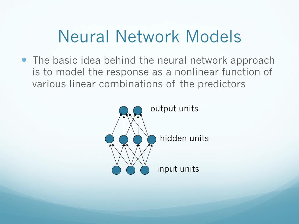
Neural Network Models �  The basic idea behind the neural network approach

is to model the response as a nonlinear function of various linear combinations of the predictors

hidden units

output units

input units

Types of Neurons

�  Linear

�  Binary threshold

�  Rectified Linear

�  Sigmoid

Perceptron �  One of the earliest

algorithms for linear classification (Rosenblatt, 1958)

�  Based on finding a separating hyperplane of the data

Perceptron Architecture �  Manually engineer features; mostly based on

common sense and hand-written programs.

�  Learn how to weight each of the features to get a single scalar quantity.

�  If this quantity is above some threshold, decide that the input vector is a positive example of the target class.

Perceptron Algorithm �  Add an extra component with value 1 to each input vector. The “bias” weight on this component is minus the threshold. Now we can have the threshold set to zero.

�  Pick training cases using any policy that ensures that every training case will keep getting picked. �  If the output unit is correct, leave its weights alone. �  If the output unit incorrectly outputs a negative class, add the

input vector to the weight vector. �  If the output unit incorrectly outputs a positive class, subtract

the input vector from the weight vector.

�  This is guaranteed to find a set of weights that gets the right answer for all the training cases if any such set exists.

Perceptron Updates

wnew = wold + x

Perceptron Updates

wnew = wold − x

Perceptron Convergence �  Theorem (Block, 1962, and Novikoff, 1962).

�  Let a sequence of examples

be given. Suppose that for all , and further that there exists a unit-length vector such that for all examples in the sequence.

Then the total number of mistakes that the algorithm makes on this sequence is at most

(x(1), y(1) ), (x(2), y(2) ),....(x(m), y(m) )|| x(i) || ≤ D i

u (|| u ||2=1)y(i).(uT x(i) ) ≥ γ

D γ( )2

Chapter 1: Deep Architectures

Limitations of Perceptron

�  There is no value for W and b such that the model results in right target for every example

x1

x2

y

W, b

0,1

0,0 1,0

1,1

weight plane output =1 output =0

A graphical view of the XOR problem

Learning representations

0,0 1,0

2,1

x2

x1 u1

u2 h2

h1

y

W, b φV, c

W =1111⎡

⎣⎢

⎤

⎦⎥, b =

0−1⎡

⎣⎢

⎤

⎦⎥, V =

1−2⎡

⎣⎢

⎤

⎦⎥ and c = 0

�  Theorem: A neural network with one hidden layer can approximate any continuous function.

�  More formally, given a continuous function where is a compact subset of ,

such that

f :Cn ! Rm

Cn Rn

∀ε, ∃ fNNε : x→ Viφ(WT

ii=1

K

∑ + bi )+ c

∀x ∈Cn, f (x)− f εNN (x) < ε

Universal Approximation

Universal Approximation �  Cybenko 1989; Hornik et al., 1989 proved the

universal approximation properties for networks with squashing activation function such as logistic sigmoid.

�  Leshno et al., 1993 proved the UA properties for Rectified Linear Unit activation functions.

Deep vs Shallow �  Pascanu et al. (2013) compared deep rectifier

networks with their shallow counterparts. �  For a deep model with inputs and hidden layers

of width , the maximal number of response regions per parameter behaves as

�  For a shallow model with inputs and hidden units, the maximal number of response regions per parameter behaves as

n0 kn

Ωnn0

⎢

⎣⎢

⎥

⎦⎥

k−1nn0−2

k

⎛

⎝⎜⎜

⎞

⎠⎟⎟

O kn0−1nn0−1( )

n0 nk

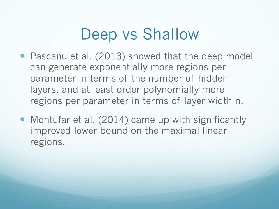
Deep vs Shallow �  Pascanu et al. (2013) showed that the deep model

can generate exponentially more regions per parameter in terms of the number of hidden layers, and at least order polynomially more regions per parameter in terms of layer width n.

�  Montufar et al. (2014) came up with significantly improved lower bound on the maximal linear regions.

Chapter 2: Feed-forward Neural Networks

Feed-forward neural networks �  These are the commonest type of

neural network in practical applications.

�  The first layer is the input and the last layer is the output.

�  If there is more than one hidden layer, we call them “deep” neural networks.

�  They compute a series of transformations that change the similarities between cases.

�  The activities of the neurons in each layer are a non-linear function of the activities in the layer below.

hidden units

output units

input units

Backpropagation

�  First convert the discrepancy between each output and its target value into an error derivative.

�  Then compute error derivatives in each hidden layer from error derivatives in the layer above.

�  Then use error derivatives w.r.t. activities to get error derivatives w.r.t. the incoming weights.

E = 12

(t jj∈output∑ − yj )

2

∂E∂yj

= −(t j − yj )

∂E∂yj

∂E∂yi

Backpropagation

∂E∂z j

=dyjdz j

∂E∂yj

= yj (1− yj )∂E∂yj

yjj

yii

z j

∂E∂yi

=dzjdyi

∂E∂z jj

∑ = wij∂E∂z jj

∑

∂E∂wij

=∂z j∂wij

∂E∂z j

= yi∂E∂z j

E = 12

(t jj∈output∑ − yj )

2

∂E∂yj

= −(t j − yj )

References �  Yoshua Bengio, Learning deep architecures for AI:

http://www.iro.umontreal.ca/~bengioy/papers/ftml_book.pdf

�  Geoff Hinton, Neural networks for machine learning: https://www.coursera.org/learn/neural-networks

�  Goodfellow et al., Deep Learning: http://www.deeplearningbook.org/

�  Montufar et al., On the number of linear regions of Deep Networks: https://arxiv.org/pdf/1402.1869.pdf

References �  Pascanu et al., On the number of response regions of

deep feed forward neural networks with piece-wise linear activations: https://arxiv.org/pdf/1312.6098.pdf

�  Perceptron weight update graphics:https://www.cs.utah.edu/~piyush/teaching/8-9-print.pdf

�  Proof of Theorem (Block, 1962, and Novikoff, 1962).http://cs229.stanford.edu/notes/cs229-notes6.pdf