NBER WORKING PAPER SERIES

COMPARATIVE ADVANTAGE, LEARNING,

AND SECTORAL WAGE DETERMINATION

Robert Gibbons

Lawrence F. Katz

Thomas Lemieux

Daniel Parent

Working Paper 8889

http://www.nber.org/papers/w8889

NATIONAL BUREAU OF ECONOMIC RESEARCH

1050 Massachusetts Avenue

Cambridge, MA 02138

April 2002

We thank Derek Neal for persistently encouraging this project during much of its 13-year gestation, David

Card for helpful comments that inspired its completion, and the NSF (Gibbons and Katz) and SSHRC

(Lemieux and Parent) for financial support. The views expressed herein are those of the authors and not

necessarily those of the National Bureau of Economic Research.

© 2002 by Robert Gibbons, Lawrence F. Katz, Thomas Lemieux and Daniel Parent. All rights reserved.

Short sections of text, not to exceed two paragraphs, may be quoted without explicit permission provided

that full credit, including © notice, is given to the source.

Comparative Advantage, Learning, and Sectoral Wage Determination

Robert Gibbons, Lawrence F. Katz, Thomas Lemieux and Daniel Parent

NBER Working Paper No. 8889

April 2002

JEL No. J3

ABSTRACT

We develop a model in which a worker's skills determine the worker's current wage and sector.

Both the market and the worker are initially uncertain about some of the worker's skills. Endogenous

wage changes and sector mobility occur as labor-market participants learn about these unobserved skills.

We show how the model can be estimated using non-linear instrumental-variables techniques. We then

apply our methodology to study the wages and allocation of workers across occupations and across

industries. For both occupations and industries, we find that high-wage sectors employ high-skill workers

and offer high returns to workers' skills. Estimates of these sectoral wage differences that do not account

for sector-specific returns are therefore misleading. We also suggest further applications of our theory

and methodology.

Robert Gibbons Lawrence F. Katz

Sloan School of Management Department of Economics

and Department of Economics Harvard University

MIT Cambridge, MA 02138

Cambridge, MA 02142 and NBER

and NBER lkatz@harvard.edu

rgibbons@mit.edu

Thomas Lemieux Daniel Parent

Department of Economics Department of Economics

University of British Columbia McGill University

Vancouver, BC V6T 1Z1 Montreal H3A 2T7

Canada Canada

and NBER dparent@arts22911.arts.mcgill.ca

tlemieux@interchange.ubc.edu

1. Introduction

We analyze the theoretical and econometric implications of comparative advantage and

learning for the wages and sector affiliations of individuals, and for changes in these variables

over workers’ careers. After developing the theory and econometrics, we turn to two empirical

applications of our methodology, concerning the wages and allocations of workers across

occupations and across industries.

Our focus on comparative advantage is motivated by a large and established literature.

Many have found that the average characteristics of individuals vary by sector.1 Furthermore,

several have found that the measured returns to individuals’ observable characteristics vary by

sector.2 Finally, Heckman and Scheinkman (1987) rejected the hypothesis that the returns to

individuals’ time-invariant unmeasured characteristics are constant across sectors.

Our focus on learning is motivated by a smaller and more recent literature. While

Jovanovic (1979), Harris and Holmstrom (1982), and others showed long ago that learning

models could provide new interpretations for important features of the data (such as the return to

seniority and the increase in the variance of wages with experience), recent work has built on

these foundations to derive and test novel implications, many of which have survived

confrontations with data.3

Our theoretical model emphasizes the role of worker skills that cannot be measured by an

econometrician. To clarify the exposition of the econometrics, we develop the theory in stages.

1 For example, Dickens and Katz (1987) found differences in average education levels by industry and Blackburn and Neumark (1992) found sorting by test scores across industries. 2 For example, Mincer and Higuchi (1988) found differences in returns to tenure and experience across industries in Japan and the US and Freeman and Medoff (1984) found differences in returns to education and experience for union and non-union workers. 3 For example, Farber and Gibbons (1996) derive and test the prediction that the residual from a regression of an individual’s score on an ability test (AFQT) on observable characteristics and the first wage should have increasing explanatory power for subsequent wages as experience increases. Continuing in this vein, Altonji and Pierret (2001) derive and test the prediction that the effect of observable characteristics (like education) should decrease with experience while the effect of initially unobservable characteristics like AFQT (not only the AFQT residual) should increase with experience. Chiappori, Salanié, and Valentin (1999) derive and test a new prediction from the Harris-Holmstrom model, that comparing two individuals in the same job in period 1 and the same (higher) job in period 3, future wage and promotion prospects are brighter for the individual who was promoted later (i.e., in period 3 rather than period 2).

1

We begin with two models in which workers’ skills are equally valued in all sectors. In the first

of these models, all labor-market participants have perfect information about workers’ skills; in

the second, information is initially imperfect but output observations convey additional

information over time and so endogenize wage changes. We then develop two other models in

which different sectors place different values on workers’ skills and workers sort themselves into

different sectors on the basis of comparative advantage. In the first of these latter two models,

labor-market participants again have perfect information about workers’ skills; in the second,

information is again imperfect, so learning endogenizes not only wage changes but now also

sector mobility.

Our richest model, with comparative advantage and learning, resembles the learning and

matching models of wages and turnover pioneered by Jovanovic (1979), Ross, Taubman, and

Wachter (1981), and MacDonald (1982). In Jovanovic's model, a worker's performance is

independent across jobs, whereas in our model (like Ross et. al. and MacDonald), a worker's

performance in one job determines not only the expected value of staying in that job but also the

expected value of moving to a given new job. We differ from Ross et. al. and MacDonald by

introducing a one-dimensional notion of ability that determines a worker’s productivity in every

sector, much as in Murphy (1986). The resulting model of learning and sorting is a natural

generalization of the two-period, two-sector, two-type model in Gibbons and Katz (1992).

As is well known, in our simplest theoretical model (in which worker skills are equally

valued in all sectors and there is no learning by labor-market participants), the returns to time-

varying worker characteristics can be estimated using first-differences to eliminate individual

fixed effects that are unmeasured by the econometrician. Similarly, in this simplest model, first-

differences can be used to estimate sectoral wage differentials without bias from unmeasured

fixed effects. Unfortunately, first-difference estimation is not appropriate for any of the three

other theoretical models we develop. Simply put, in these models, a worker’s fixed ability does

not translate into a fixed effect in a wage equation, so first-differencing the wage equation does

2

not correct ability bias. The contribution of this paper is to move beyond merely warning of this

problem (as in Gibbons and Katz, 1992, for example) to proposing a solution.

Our theoretical models rely heavily on the assumption of normality. Many models that

rely on normality can be estimated by maximum likelihood or by two-step methods, but

estimating our dynamic model of wage determination and sector affiliation would be

computationally difficult because it entails more than two sectors and more than two periods. In

addition, it is not necessary to estimate the full model when the parameters of interest are those

that determine the returns to skills and wage differences across sectors. We therefore undertake

the more modest task of estimating the wage equations in each sector.4

We show that our richest theoretical model produces a random-coefficients econometric

model in a panel-data setting, which can be estimated using a non-linear instrumental-variables

technique. Even in this richest model, consistent estimates of the effects of both measured and

unmeasured skills on wages require neither distributional assumptions nor standard exclusion

restrictions. (That is, we use normal distributions to develop the full theory, but we do not need

these assumptions to estimate the parameters of interest related to sectoral wage differentials and

sector-specific returns to skills.) Instead, the estimation strategy utilizes natural restrictions

available in panel data with three or more observations per person. Our econometric approach is

similar to other panel-data models in which first-differenced estimates are inconsistent, such as

Holtz-Eakin, Newey, and Rosen (1988) and Lemieux (1998).

After developing the theory and econometrics, we implement two empirical

investigations, concerning sorting and wage differentials across occupations and industries,

using individual-level panel data from the National Longitudinal Survey of Youth. Our richest

theoretical model is consistent with several familiar facts about wage determination: a typical

individual’s wage increases with experience, the variance of the wage distribution across

4 Other results exist on the identifiability of related models in the absence of normality. For example, Heckman and Honore (1990) show that the Roy model is identified with panel data and exogenous shifts in the price of skills over time. But Heckman and Honore focus on the estimation of a sequence of static models; they do not address learning and job mobility.

3

individuals increases with experience, and the skewness of the wage distribution increases with

experience.5 But variants of Mincer’s (1974) theory can also explain these basic facts, so we

focus on our model’s further predictions, concerning the returns to skills and the resulting

allocation of workers across sectors. For both occupations and industries, we find important

variation in sector-specific returns to observed and unobserved skills. Furthermore, in both cases,

high-wage sectors employ high-skill workers and offer high returns to workers’ skills, so

estimates of sectoral wage differences that do not account for sector-specific returns to skill and

the sorting of workers across sectors on the basis of unmeasured skills are misleading and

difficult to interpret.

Although our empirical work explores two standard definitions of sectors (namely,

occupations and industries), other definitions are possible. For example, sectors could be jobs

inside a firm (Gibbons and Waldman, 1999; Lluis, 2001), states or regions within a country

(Borjas, Bronars, and Trejo, 1992), or entire countries (Borjas, 1987). In fact, the individuals in

our model need not be workers. Instead, they could be firms, where what we call worker ability

is reinterpreted as firm productivity, much as Jovanovic (1982) reinterpreted Jovanovic (1979).

2. Theory and Econometrics

The four theoretical models analyzed below are special cases of the following model. If

worker i is employed in sector j at time t, the worker's output is

(1) yijt = exp(Xit βj + ψijt),

where Xit is a vector of human-capital and demographic variables measured by the

econometrician and ψijt represents determinants of productivity that are not measured by the

econometrician. The worker characteristics Xit and the slope vector βj are known by all labor- 5 An illustrative discussion of these implications of the model and a comparison with alternative labor market models is presented in Neal and Rosen (2000).

4

market participants at the beginning of period t; the realized output yijt is observed by all labor-

market participants at the end of period t. The error term ψijt has the components

(2) ψijt = Zi + bj (ηi + εijt ) + cj,

where Zi denotes the portion of worker i’s productive ability that is equally valued in all sectors,

ηi denotes the portion that is differentially valued across sectors, and εijt is a random error. The

coefficients {bj, cj : j = 1,...,J} are fixed and known to all labor-market participants. The noise

terms εijt are normal with zero mean and precision hε (i.e., variance σε2 = 1/hε ) and are

independent of each other and of all the other random variables in the model.

In developing the theory and econometrics, we treat Zi and ηi differently. We assume

throughout that Zi is observed by all labor-market participants; this is the standard case of a fixed

effect that the econometrician cannot observe but market participants can. For ηi, however, we

consider two cases: perfect information (no learning by market participants, as with Zi) and

imperfect information (learning). One could also imagine investigating learning about Zi. Farber

and Gibbons (1996) study this problem in the absence of sector-specific returns to ability (i.e.,

bj=b and βj = β for every j, so that a worker's unmeasured ability is Zi + bηi and is equally valued

in every sector), but the combined problem of learning about Zi and about ηi awaits future

research.

In the imperfect-information case, all labor-market participants share symmetric but

imperfect information about ηi. In particular, given their initial information (Zi and Xi1), all

participants in the labor market share the prior belief that ηi is normal with mean m and precision

h. Subsequent productivity observations, yijt , refine this belief. Information in the labor market

therefore remains symmetric and improves over time. For simplicity, we assume that subsequent

realizations of measured skills, Xit, are conditionally independent of ηi given Zi and Xi1. (This

assumption is not only convenient but realistic, because the major time-varying element of Xit is

experience.) Thus, market participants can compute

5

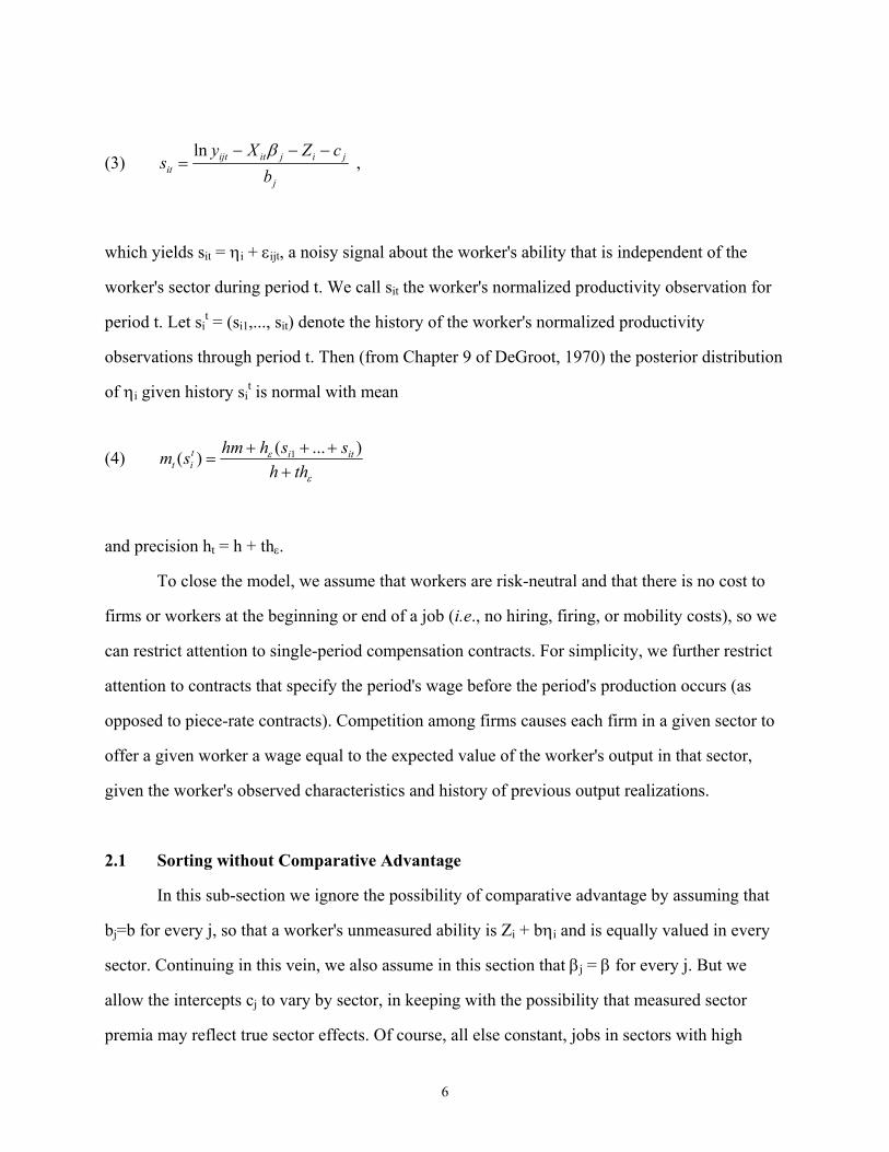
(3) j

jijitijtit b

cZXys

−−−=

βln ,

which yields sit = ηi + εijt, a noisy signal about the worker's ability that is independent of the

worker's sector during period t. We call sit the worker's normalized productivity observation for

period t. Let sit = (si1,..., sit) denote the history of the worker's normalized productivity

observations through period t. Then (from Chapter 9 of DeGroot, 1970) the posterior distribution

of ηi given history sit is normal with mean

(4) ε

ε

thhsshhmsm itit

it ++++

=)...()( 1

and precision ht = h + thε.

To close the model, we assume that workers are risk-neutral and that there is no cost to

firms or workers at the beginning or end of a job (i.e., no hiring, firing, or mobility costs), so we

can restrict attention to single-period compensation contracts. For simplicity, we further restrict

attention to contracts that specify the period's wage before the period's production occurs (as

opposed to piece-rate contracts). Competition among firms causes each firm in a given sector to

offer a given worker a wage equal to the expected value of the worker's output in that sector,

given the worker's observed characteristics and history of previous output realizations.

2.1 Sorting without Comparative Advantage

In this sub-section we ignore the possibility of comparative advantage by assuming that

bj=b for every j, so that a worker's unmeasured ability is Zi + bηi and is equally valued in every

sector. Continuing in this vein, we also assume in this section that βj = β for every j. But we

allow the intercepts cj to vary by sector, in keeping with the possibility that measured sector

premia may reflect true sector effects. Of course, all else constant, jobs in sectors with high

6

values of cj may be more attractive (depending on the source of cj , such as rent-sharing versus

compensating differentials). If some sectors are more attractive, issues such as queuing and

rationing arise. Because our main interest is in the richer model with comparative advantage in

Section 2.3, we do not formally address queuing or rationing here.

It is not controversial that workers' productive abilities are imprecisely measured in

standard micro data sets. But if unmeasured skills are to explain estimated sector wage

differentials then these skills must be non-randomly allocated across sectors. This, too, is

plausible, for example because different sectors use different technologies that require workers'

skills in different proportions. But if this unmeasured-skill explanation for measured sectoral

wage differentials is correct, it suggests that the few skills that are measured in standard micro

data sets (hereafter "measured skills") should be systematically related to the sector in which the

worker is employed. We investigate this prediction about measured skills in our empirical work

on occupations and industries in Sections 3 and 4. For now, however, we confine our attention to

econometric approaches to estimating the role of unmeasured skills.

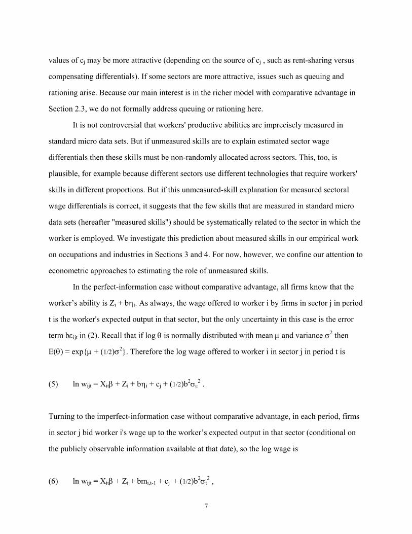
In the perfect-information case without comparative advantage, all firms know that the

worker’s ability is Zi + bηi. As always, the wage offered to worker i by firms in sector j in period

t is the worker's expected output in that sector, but the only uncertainty in this case is the error

term bεijt in (2). Recall that if log θ is normally distributed with mean µ and variance σ2 then

E(θ) = exp{µ + (1/2)σ2}. Therefore the log wage offered to worker i in sector j in period t is

(5) ln wijt = Xitβ + Zi + bηi + cj + (1/2)b2σε2 .

Turning to the imperfect-information case without comparative advantage, in each period, firms

in sector j bid worker i's wage up to the worker’s expected output in that sector (conditional on

the publicly observable information available at that date), so the log wage is

(6) ln wijt = Xitβ + Zi + bmi,t-1 + cj + (1/2)b2σt2 ,

7

where mi,t-1 is shorthand for mt-1(sit-1) and σt

2 = [h + thε]/(hε[h + (t-1)hε]). In both the perfect- and

the imperfect-information cases, the worker's ability ηi is unmeasured by the econometrician (as

is Zi); in the latter case, ηi is also unobserved by labor-market participants (unlike Zi). Note that,

since t represents the number of years of experience in the model, the error component (1/2)b2σt2

will be captured by a linear function in labor market experience that we include in all estimated

models.

2.2 Estimation without Comparative Advantage

In the absence of both learning and comparative advantage, the source of possible bias in

conventional cross-section estimates of sectoral log wage differentials is the potential partial

correlation between sector affiliation and unmeasured skills (Zi and ηi) conditional on measured

skills (Xit). In this simplest case, the worker’s fixed ability (Zi + bηi) creates a worker fixed-

effect in the wage regression, which can be eliminated in standard fashion. For example, a first-

differenced regression eliminates the fixed effect Zi + bηi in (5).

Even without comparative advantage, however, learning implies that fixed ability is not a

fixed effect in the earnings equation. The key property of our learning model is that Bayesian

beliefs are a martingale. That is, the conditional expectation mt(sit) in (4) obeys the law of motion

(7) mit = mi,t-1 + ξit,

where ξit is a noise term orthogonal to mi,t-1. In somewhat more intuitive terms, the market begins

period t with the information contained in sit-1 and then extracts new information about ηi from

the output observation yijt (or, equivalently, sit). But the new information that can be extracted

from yijt is precisely the part that could not be forecasted from sit-1. Hence, the innovation ξit is

orthogonal to the prior belief mi,t-1.

8

Farber and Gibbons (1996) explored some of the implications of this martingale property.

But they focused on several specific predictions that can be derived regarding regressions in

which the dependent variable is the level of earnings, not the log of earnings. In this paper, in

contrast, we use the log of earnings as the dependent variable, so the specific Farber-Gibbons

predictions do not hold, but the martingale property of the market's beliefs continues to create

endogeneity problems, as follows.6

Formally, a first-differenced regression eliminates Zi but not mi,t-1 from (6). Instead, first-

differencing (6) for a worker who switches from sector j to sector j' yields

(8) ln wit - ln wi,t-1 = (Xit - Xi,t-1)β + b(mi,t-1 - mi,t-2) + (cj' - cj) + (1/2)b2(σt2 - σ2

t-1) ,

where mi,t-1 - mi,t-2 = ξi,t-1. But ξi,t-1 may be correlated with the change in sector affiliation through

whatever (unmodeled) process led unmeasured ability to be correlated with sector affiliation in

the first place.7 Thus, with learning, first-differenced estimates of sectoral wage differentials are

biased if the change in the residual is correlated with the change in sector affiliation. Fortunately,

this endogeneity problem is simple to correct because the new information summarized in ξi,t-1 is

not related to wage, skill, or sector information in period t - 1 or earlier. (See Section 2.4 for

more discussion of this issue.) For example, equation (8) can be estimated by two-stage least

squares using the interaction of the worker’s score on an ability test (taken before the worker

entered the labor market) and the worker’s sector affiliation at t-1 as a valid instrumental

variable for changes (between t - 1 and t) in sector affiliation. 6 Relative to Farber and Gibbons, we also use the more specific production function (1), the more specific error structure (2), and the more specific distributional assumptions given in the text below (2). We impose these more specific assumptions in order to explore several issues related to the returns to skills across sectors, which Farber and Gibbons could not address with their more general model. 7 For example, suppose that there are only two levels of ability, high and low, but that sectors differ in the proportion of high-ability workers they employ. Consider a high-ability worker whose employment exogenously ends in sector j. Suppose that such a worker is equally likely to be re-employed in any of the economy’s jobs for high-ability workers. Then there is some probability that the worker’s new job is again in sector j, but if the worker changes sectors then it is likely that the new job is in a sector with a large number of high-ability jobs. In this case, positive information about a worker’s ability will tend to be associated with shifts to high-wage sectors (where high-skill jobs are more plentiful), and the reverse for negative information.

9

2.3 Sorting with Comparative Advantage

In this section we relax the assumption that a worker's ability is equally valued in every

sector. By introducing comparative advantage, we endogenize sector affiliation. By subsequently

introducing learning, we endogenize not only wage changes but also sector mobility.

To analyze comparative advantage, we now return to the production function specified in

(1) and (2), where the slope coefficients βj in (1) and bj in (2) vary by sector. We index the J

sectors so that bj strictly increases in j: sector j + 1 values the worker's ability ηi more than does

sector j. In keeping with the notion that ability is productive, we assume that b1 > 0. Given a

fixed Xit there exist critical values of ηi that determine the efficient assignment of workers to

sectors. Denoting these critical values by {vj(Xit) : j = 0, 1,...,J}, the efficient assignment rule

assigns worker ηi to sector j if and only if vj-1(Xit) < ηi < vj(Xit), where v0(Xit) = -∞, vn(Xit) = ∞,

and vj(Xit) strictly increases in j. See Figure 1 for a graphical representation of this efficient

assignment rule.

We again analyze first perfect and then imperfect information. In the perfect-information

case, firms in sector j bid worker i's wage up to the expected output in that sector:

(9) ln wijt = Xitβj + Zi + bjηi + cj + (1/2)bj2σε

2 ,

analogous to (5) but with the sector-specific returns βj and bj. If the worker faces no mobility

constraints, worker i will choose to work in sector j if vj-1(Xit ) < ηi < vj(Xit). Thus, taking the

model literally, sector mobility in the perfect-information case is driven entirely by changes in

Xitβj. One could envision exogenous shocks to sector demand that produce additional sector

mobility in this model, but we will not formally model such shocks, for the same reason that we

did not model queues or rationing above: our ultimate interest is in the model with comparative

advantage and learning, which gives a coherent account of sectoral mobility without reference to

queues, rationing, or sectoral shocks. Whatever the reason that worker i is employed in sector j

10

in period t, in the perfect-information case with comparative advantage we assume that the

worker's wage is given by (9).

In the imperfect-information case, we again assume that information in the labor market

is symmetric but imperfect, as described above. As in the model of learning without comparative

advantage, all participants in the labor market share the prior belief that ηi is normal with mean

m and precision h, conditional on their initial information Zi and Xi1. Inferences from the

productivity observations, yijt, are greatly simplified because the information content of an output

observation is constant across sectors; that is, (2) involves bj(ηi + εijt) rather than bjηi + εijt. This

functional form is what allows us to define the normalized productivity observation for worker i

in period t, sit from (3), to be a noisy signal about the worker's ability that is independent of the

worker's sector during period t. Relaxing this assumption about the functional form of (2) would

complicate the analysis because workers' sector choices would then depend on the benefit from

faster learning as well as on the benefit from increased expected output given current beliefs.

Relaxing the assumption that all labor-market participants observe Zi (so that there could be

learning about both Zi and ηi) would cause similar complications. Under our assumptions, the

posterior distribution of ηi given the history sit is normal with mean mit given by (4) and

precision ht = h + thε, regardless of the worker’s history of sector affiliations.

In this fourth model, with learning and comparative advantage, we finally have an

internally consistent account for sector affiliation, wages, sector mobility, and wage changes, as

follows. In each period, firms in sector j bid a worker's wage up to the worker's expected output

in that sector, conditional on the publicly observable information about the worker available at

that date:

(10) ln wijt = Xitβj + Zi + bjmi,t-1 + cj + (1/2)bj2σt

2,

analogous to (6) but with sector-specific returns βj and bj. The model also includes sector-

specific (experience) effects since the posterior variance σt2, which declines with time (labor

11

market experience), is interacted with bj2. The worker chooses to work in the sector offering the

highest current wage. Thus, worker i chooses sector j in period t+1 if vj-1(Xit ) < mit < vj(Xit).

2.4 Estimation with Comparative Advantage

We now develop a non-linear instrumental-variables procedure to estimate the

parameters {βj, bj, cj; j = 1,..., J} in (9) and (10). This procedure does not rely on normality and

can be implemented using standard computer packages. To discuss the estimation of the model,

define the sector indicators Dijt where:

Dijt = 1 if person i is employed in sector j at time t,

Dijt = 0 otherwise.

The wage equation (10) for each sector j can then be written as a single equation where

measurement error µit is assumed to be independent of sector affiliation:

(11) itj

tjijtj

tijijtj

ijitijtj

jijtit bDmbDZXDcDw µσβ ∑∑∑∑ +++++= −22

1, )(ln 1/2 .

Estimates of the sector slopes and intercepts {βj, cj; j = 1,..., J} obtained by estimating equation

(11) with OLS are inconsistent. The problem is that expected ability influences sector affiliation,

so mi,t-1 is correlated with the set of sector dummies {Dijt, j = 1,..., J}.

The endogeneity problem in equation (11) is different from the usual fixed-effect case for

two reasons. First, as noted in Section 2.2, mi,t-1 is a martingale rather than a fixed effect. This

martingale property does not depend on the normality assumptions in our theoretical model; all

Bayesian beliefs are martingales. In the absence of comparative advantage, we could handle this

martingale problem as described in Section 2.2. But, second, comparative advantage causes mi,t-1

to be interacted with the set of sector dummies {Dijt, j = 1,..., J} in (11).

Other panel-data models in which first-differenced estimates are inconsistent have been

considered in the literature. For example, Holtz-Eakin, Newey, and Rosen (1988) discuss the

12

estimation of models in which the fixed effect is interacted with year dummies. They show that

consistent estimates can be obtained by quasi-differencing the equation of interest and then using

appropriate instrumental-variables techniques. Similarly, Lemieux (1998) estimates a model in

which the return to a time-invariant unobserved characteristic is different in the union and the

nonunion sectors.

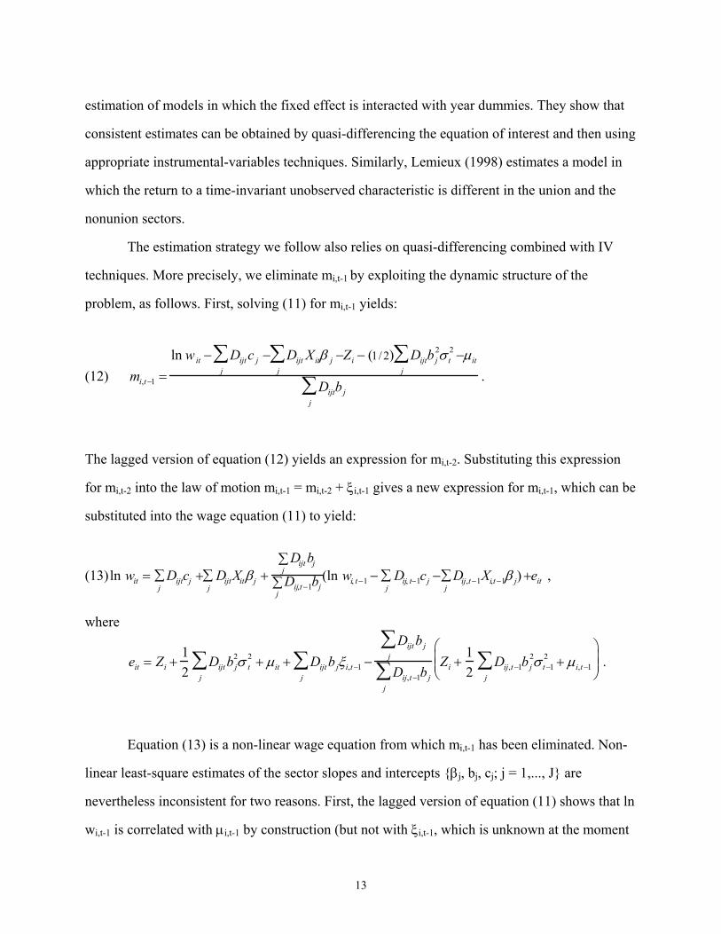
The estimation strategy we follow also relies on quasi-differencing combined with IV

techniques. More precisely, we eliminate mi,t-1 by exploiting the dynamic structure of the

problem, as follows. First, solving (11) for mi,t-1 yields:

(12) mi,t −1 =ln wit − Dijtc j −

j∑ Dijt Xitβ j −

j∑ Zi − (1/2) Dijtb j

2σ t2 −

j∑ µit

Dijtb jj

∑ .

The lagged version of equation (12) yields an expression for mi,t-2. Substituting this expression

for mi,t-2 into the law of motion mi,t-1 = mi,t-2 + ξi,t-1 gives a new expression for mi,t-1, which can be

substituted into the wage equation (11) to yield:

(13) ln wit = Dijtcj +j∑ DijtXitβj +

Dijtbjj∑

Dij,t −1bjj∑j

∑ (ln wi, t −1 − Dij, t−1cj −j

∑ Dij,t −1Xi,t −1β j) +j∑ eit ,

where

. eit = Zi +12

Dijtb j2σ t

2

j∑ + µit + Dijt

j∑ bjξi,t −1 −

Dijtb jj

∑Dij,t −1bj

j∑ Zi +

12

Dij,t −1bj2

j∑ σ t −1

2 + µi,t −1

Equation (13) is a non-linear wage equation from which mi,t-1 has been eliminated. Non-

linear least-square estimates of the sector slopes and intercepts {βj, bj, cj; j = 1,..., J} are

nevertheless inconsistent for two reasons. First, the lagged version of equation (11) shows that ln

wi,t-1 is correlated with µi,t-1 by construction (but not with ξi,t-1, which is unknown at the moment

13

wi,t-1 is decided). Second, the sector dummies Dijt are correlated with νi,t-1 because expected

ability influences sector affiliation. Fortunately, both of these problems can be handled by

finding appropriate instruments for ln wi,t-1 and the set of sector dummies {Dijt, j = 1,..., J}. Such

instrumental variables must of course be independent of the error term eit in equation (13).

The most obvious candidate instrumental variables are wage, skill, or sector information

from period t-1 or earlier, as well as interactions of these variables. Since the evolution of wages

and sector affiliation over time is driven by the evolution of mit, these wage, skill, and sector

histories should help predict mi,t-1 and thus ln wi,t-1 and {Dijt, j = 1,..., J}. We chose the

interaction between sector affiliation at time t-1 and t-2, {Dij,t-1, j = 1,..., J} and {Dij,t-2, j = 1,...,

J}, as our main instrumental variables. These interactions between sector affiliation at t-1 and t-

2 are uncorrelated with the error term eit in equation (13) given the model’s assumption that

sector affiliation is determined only by perceptions about the sector-sensitive components of

ability (Xit and ηi) and is independent of any part of ability that is not differentially valued across

sectors (Zi). In Appendix B we discuss in more detail why the model suggests using these

variables as instruments. We also show evidence of their predictive power. For efficiency

reasons discussed below, we also include a set of interactions of sector affiliation at time t-2 with

the explanatory variables Xit (as summarized by a skill index and year of experience) in the

instrument set.8

We estimate the parameters in equation (13) using non-linear instrumental-variables

(NLIV) techniques. Consider e, a vector in which all the individual error terms eit are stacked,

and V, a matrix in which the individual instrument vector vit (e.g., sector histories) are stacked.

Since the error terms e should be uncorrelated with the instruments V, the orthogonality

condition (1/N)e'V = 0 should hold. The NLIV method consists of setting the sample analogs of

8 Since both the terms Xitβj and (1/2)bj

2σt2 are interacted with sector affiliation, which is endogenous, it is

natural to include some instruments for sector affiliation interacted with those terms in the instrument set. In the estimation we replace Xitβj by a skill index discussed below and use experience to proxy for σt

2. This leads to adding interactions between the second lag of sector affiliation (the instruments for sector affiliation) and the skill index and experience to the main set of instruments (interactions between sector affiliation at t-1 and t-2).

14

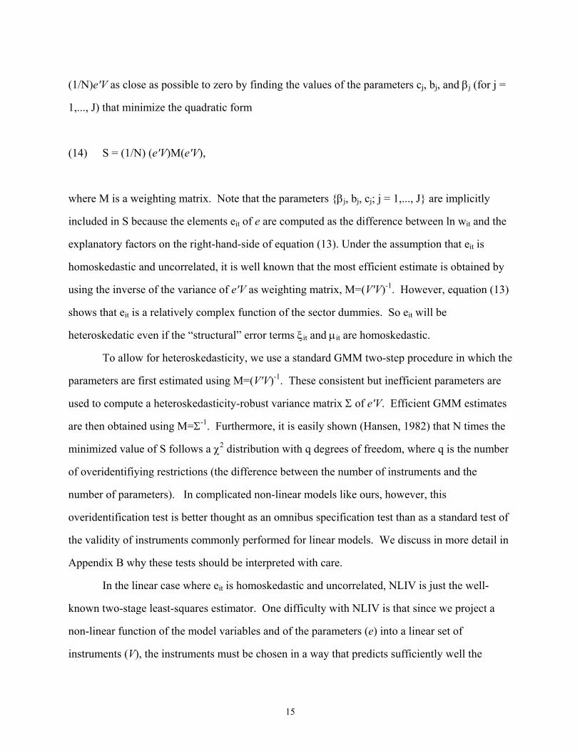
(1/N)e'V as close as possible to zero by finding the values of the parameters cj, bj, and βj (for j =

1,..., J) that minimize the quadratic form

(14) S = (1/N) (e'V)M(e'V),

where M is a weighting matrix. Note that the parameters {βj, bj, cj; j = 1,..., J} are implicitly

included in S because the elements eit of e are computed as the difference between ln wit and the

explanatory factors on the right-hand-side of equation (13). Under the assumption that eit is

homoskedastic and uncorrelated, it is well known that the most efficient estimate is obtained by

using the inverse of the variance of e'V as weighting matrix, M=(V'V)-1. However, equation (13)

shows that eit is a relatively complex function of the sector dummies. So eit will be

heteroskedatic even if the “structural” error terms ξit and µit are homoskedastic.

To allow for heteroskedasticity, we use a standard GMM two-step procedure in which the

parameters are first estimated using M=(V'V)-1. These consistent but inefficient parameters are

used to compute a heteroskedasticity-robust variance matrix Σ of e'V. Efficient GMM estimates

are then obtained using M=Σ-1. Furthermore, it is easily shown (Hansen, 1982) that N times the

minimized value of S follows a χ2 distribution with q degrees of freedom, where q is the number

of overidentifiying restrictions (the difference between the number of instruments and the

number of parameters). In complicated non-linear models like ours, however, this

overidentification test is better thought as an omnibus specification test than as a standard test of

the validity of instruments commonly performed for linear models. We discuss in more detail in

Appendix B why these tests should be interpreted with care.

In the linear case where eit is homoskedastic and uncorrelated, NLIV is just the well-

known two-stage least-squares estimator. One difficulty with NLIV is that since we project a

non-linear function of the model variables and of the parameters (e) into a linear set of

instruments (V), the instruments must be chosen in a way that predicts sufficiently well the

15

explanatory righthand side of equation (13).9 In addition to the sector histories discussed above,

we thus include as instruments a set of interactions between the explanatory variables Xit (as

summarized by a skill index and years of experience) and the period t - 2 dummies for sector

affiliation {Dij,t-2, j = 1,..., J}.

In the perfect-information case, where unmeasured ability ηi is observed by labor market

participants, the quasi-differenced equation (13) remains the same except that the innovation

term ξi,t-1 drops from the error term eit. The remaining endogeneity problem is due to the

correlation between ln wi,t-1 and the error component µi,t-1. In this case, we simply use the full set

of interactions between the sector dummies at time t and t - 1 as instruments for ln wi,t-1.10

3. Data

The data set used in this paper is the National Longitudinal Survey of Youth, or NLSY.

Individuals in the NLSY were between the ages of fourteen and twenty-one on January 1, 1979.

We use up to seventeen yearly observations per worker (from 1979 to 1996).11 One advantage of

the NLSY is that it allows us to follow workers from the time they make their first long-term

transition to the labor force.

We use the same sample-selection criteria as those used by Farber and Gibbons (1996).

We classify individuals as having made a long-term transition to the labor force when they spend

at least three consecutive years primarily working, following a year spent primarily not working.

Someone is classified as primarily working if she/he has worked at least half the weeks since the

9 See Newey (1990) for more discussion and proposed (nonparametric) solutions to this problem. Note that choosing the functional form or the number of instruments can also be problematic in the linear model (Donald and Newey, 1999). 10 In the absence of learning, either the interactions between sector affiliation at time t and t-1 or at time t-1 and t-2 can be used as instruments. In practice, this choice has little impact on the results since both sets of instruments predict very well the wage (see Appendix B). Since sector affiliation is exogenous in this model, we do not need to include the additional interaction terms between the skill index, experience, and sector affiliation at time t-2 discussed above. Note that Lemieux (1998) uses an identical strategy to estimate union wage differentials when unmeasured ability is known to all labor-market participants but is differently rewarded in the union and non-union sectors: the interaction between the union status at time t and t - 1 is used as an instrument for the lagged wage. 11 There was no interview in 1995.

16

last interview and averaged at least thirty hours per week during the working weeks. Note that

the “last interview” does not necessarily refer to the previous calendar year if an individual had

not been interviewed the year before. Self-employed workers are deleted, as are members of the

NLSY military subsample. Readers are referred to Appendix 1 in Farber and Gibbons (1996) for

more details on the criteria used to construct our NLSY sample.

Farber and Gibbons used NLSY data from 1979 to 1991 interview years, whereas our

data are through 1996. Except for the longer sampling frame, the only noteworthy difference

between our sample and Farber and Gibbons’s has to do with union coverage in 1994. For some

reason, the question on union coverage in the current or most recent job at interview time (job

number 1 in the work history file) was not asked in that year. Although the error was caught and

fixed during the field period, many respondents were simply not asked this question even though

they should have been. Consequently, the raw data shows a large number “valid skips”.12 We

provide a correction of our own to partially fix this problem and recover quite a few of those

missing observations. More precisely, if an individual in 1994 is working for the same employer

as the one he worked for in the previous interview, we assign the value of the union coverage

dummy for the previous interview year to the current one. If the individual interviewed in 1994

has started working for a new employer since the last interview, we check to see whether she/he

is still working for that employer in 1996. If so, we assign the value of the union coverage

dummy for that year to the 1994 interview.

From this NLSY sample we focus on the subsample of observations at which the

individual was working at the interview date for at least the previous three years. This sample

restriction enables us to use the first and second lags of various variables in the estimation, as

explained in Section 2.4. We exclude workers in agricultural jobs. Since we (later) divide

manufacturing into durable and nondurable goods manufacturing, we also exclude a few workers

who hold jobs in manufacturing industries that are hard to classify as producing durable as

12 Personal communication from Steve McClaskie of the Center for Human Resource Research.

17

opposed to nondurable goods.13 We are left with a sample of 35,438 observations on 5,904

workers that satisfy these sample-selection criteria.

To summarize the relationship between the wage premia and observable skills, we

construct a "skill index" for each worker. We first estimate a flexible log (hourly) wage equation

using our sample.14 The base explanatory variables used in the log wage equation are the AFQT

score, years of education, education category dummies (dropout, high school graduates, some

college, and college degree), (actual) experience, experience squared, dummy variables for race,

gender, marital status, union status, and a set of dummies for year, industry, and occupation. We

also include sets of pairwise interactions between the education category dummies, gender, and

race, as well as interactions between gender and experience, gender and marital status, and race

and experience. Detailed regression results are reported in Appendix Table A with and without

the AFQT variable included.

We then use the estimated coefficients from that equation to predict the wage of each

worker. The skill index is the predicted wage based solely on the education, experience, and

AFQT score of the worker. That is, although characteristics such as occupation, industry, union

status, and demographic characteristics are included in the initial wage equation, they are not

used to construct the skill index for the worker. We normalize the skill index to have zero mean.

4. Wages and Returns to Skills Across Occupations

We believe that the concepts of sorting and comparative advantage are likely to play a

more important role for occupations than for industries, so we first estimate our models for

occupations. As we mention in Section 5, other factors such as compensating wage differences

and rent-sharing may mask the importance of comparative advantage in the case of industries.

Furthermore, our one-factor model is well suited to cases where there is a natural ordering of

13 These industries are: stone, clay, and glass; tobacco manufacturing; leather and leather products; and not specified manufacturing. Workers in these industries represent less than one percent of the full sample. 14 The wage variable in all estimated models is the hourly wage on the current job at the time of the survey.

18

sectors from least skill-sensitive to most skill-sensitive. We believe this ordering is more likely

apply to occupations (e.g. going from operatives to craft workers to managers) than industries.

4.1 Occupational Wage Premia without Comparative Advantage

Throughout the paper, we divide workers into seven conventional occupation

aggregates.15 In Table 1 we report the raw occupation log wage differentials (relative to the

service occupation) and the average values of measured skills (education and experience) and

other measured characteristics (race, sex, and marital status) by occupation. As is well known,

there are large differences across occupations in mean wages and in mean values for education

and other characteristics. There is also a strong link between these two variables: the correlation

between the raw wage premium and the mean level of education is 0.81 (bottom row of Table 1).

The mean skill index for each occupation is reported in Column 7. In keeping with the

positive correlation between the wage premium and mean education, we find that the correlation

between the raw wage premium and the mean skill index is 0.96. But the cross-occupation

variation in mean log wages in Column 1 (standard deviation of 0.181) is almost twice as large

as cross-occupation variation in the skill index in Column 7 (standard deviation of 0.099),

suggesting that there may be more to the story than just observable skills. In this spirit, Column 1

of Table 2 reports an OLS regression of the log wage on the skill index and six occupation

dummies (operatives and laborers are the base occupation). All the models reported in Table 2

also include controls for industry affiliation (nine dummy variables), gender, race, marital status,

union status, and a full set of year dummies.

The skill index is highly significant and has a coefficient of one (by construction), but the

occupation coefficients remain highly significant, although smaller than the raw wage

differentials reported in Table 1. Of course, such a regression merely replicates the common

15 Using a more detailed classification does not alter our basic findings and comes at the cost of less precise estimates of the occupation effects. Precision is an issue for the some of the non-linear instrumental variables models presented below.

19

finding that the occupation coefficients are significant even after controlling for measured

characteristics. We report it as our point of departure.

In this OLS model, the standard deviation of the estimated occupational wage premia is

.086. Column 2 reports first-differenced estimates of these premia; their standard deviation falls

to .021. Of course, these first-differenced estimates might be attenuated by false transitions. One

approach to the false-transitions problem is to estimate a fixed-effect regression rather than a

first-differenced regression.16 We present fixed-effect estimates in Column 3; the occupational

wage premia have a standard deviation of .032. Another approach to the false-transitions

problem is to re-compute the first-differenced estimates on the sub-sample of observations in

which the worker reports taking a new job (with a new employer). The resulting wage premia (in

Column 4) have a standard deviation of .036. In sum, the estimates in Columns 3 and 4 are

consistent with the view that more than half of the variation in occupational wage premia (after

controlling for measurable skills) may be due to unmeasured ability bias, even in our simplest

model without comparative advantage or learning.

In Columns 5 and 6 of Table 2 we explore the possibility of further bias associated with

learning (but not comparative advantage). As described at the end of Section 2.2, the problem is

that learning about ability may be correlated with the change in sector affiliation (such as where

job loss is exogenous but re-employment is not). As suggested in Section 2.2, we can use wage,

skill, and sector information from period t-1 or earlier to instrument for the change in sector

affiliation between periods t-1 and t. In Columns 5 and 6 we use as instruments the full set of

interactions between occupation dummies at times t-1 and t-2. For the full sample (Column 5),

none of the individual occupation effects is significant. Furthermore, the standard deviation of

the estimated occupation effects is quite small (.009), and we cannot reject that these premia are

all zero (p-value of .46). The results for the sub-sample of new jobs (Column 6) are relatively

16 Fixed-effect estimates use information from both first differences and longer differences and so are less affected by measurement error than first-difference estimates are (Griliches and Hausman, 1986).

20

similar. Now some of the estimated occupation effects are individually significant, but we still

cannot reject the null hypothesis that all premia are jointly equal to zero (p-value of 0.12).

Note that the estimates of the model for the sample of new jobs are much less precise

than when all observations are being used. As we will see in the next Section, limiting the

analysis to new jobs appears to be a much more efficient way of eliminating false transitions in

the case of industries than occupations. The problem is that people can clearly change

occupation by being promoted or re-assigned to a different task while staying with the same

employer. We lose these legitimate changes when we focus on new jobs only. By contrast, it is

much more difficult for an employee to change industry while staying with the same employer.

This means we should lose little legitimate information by focusing on new jobs in the case of

industries.

In sum, our results suggest that accounting for both unmeasured ability and learning

eliminates most of the occupational wage premia. The results in Columns 2-4 indicate that

controlling for measured and unmeasured skills explains over 80 percent of the raw standard

deviation of wages across occupations (0.181). The remaining premia are no longer significant

when learning is accounted for in Columns 5 and 6, though these results are less precise than in

the more standard models of Columns 1 to 4.

4.2 Occupational Wage Premia and Occupational Skill Premia

Our exploration of occupation wage premia without comparative advantage strongly

suggests that learning combined with the sorting of both measured and unmeasured skills

accounts for the bulk of occupational wage premia. In this section we explore the sources of this

sorting by adding comparative advantage to the analysis. We indeed find important differences

in the returns to measured and unmeasured skills across occupations. This finding suggests

caution in interpreting the standard occupational wage premia reported in Table 2 (and elsewhere

in the literature). In addition, as we describe below, such occupation-specific returns to skill

make estimated occupational wage premia difficult to interpret, even after controlling for

21

differences in returns to skills across sectors. As a result, we now shift our focus to these

differential returns to skill. In particular, we investigate whether high-skill workers are

concentrated in high-return occupations, as our theory suggests.

Table 3 extends our analysis of occupational wage premia in Table 2 by reporting not

only these premia but also occupation-specific returns to skills. All models reported in Table 3

also include the same set of additional controls (gender, race, year dummies, etc.) as in Table 2.

Column 1 of Table 3 reports OLS estimates of the wage premia, while Column 2 reports the

occupation-specific returns to observable skill. Most of the estimated returns to skill are quite

plausible. For example, all occupations but the clerical occupations have a significantly larger

return to skill than operatives and laborers. Managers and sales occupations have the largest

returns to skill, although the returns for professionals may be a bit smaller than expected.

In spite of these significant differences in occupation-specific returns to observable skills

(p-value of .00 on the joint test of equality of returns), the associated occupational wage premia

are quite similar to those from Column 1 of Table 2 (which did not allow for occupation-specific

returns to skill). For example, the standard deviation of the estimated occupational wage premia

is .096 – slightly larger than the .086 in Column 1 of Table 2. But our analysis in Table 2

suggested an important role for unmeasured skills, so we next investigate occupation-specific

returns to unobservable skills.

The remaining models reported in Columns 3 through 6 of Table 3 allow for occupation-

specific returns to both measured and unmeasured skill. In all models, we include (but do not

show in the Table) a set of interactions between occupation and experience to capture the term

(1/2)bj2σt

2 in equation (13).17 We allow returns to measured and unmeasured skill to be different

but proportional. In terms of the parameters of the model, this means that βj=kbj for all

17 Strictly speaking, this term should appear in only the learning model. We include it in all models with unmeasured skills for the sake of comparability across specifications.

22

occupations j, where k is a proportionality parameter. As we report in the tables, proportionality

can never be rejected, but k is typically statistically different from 1.18

In the first model, reported in Columns 3 and 4, we analyze the model with comparative

advantage but without learning, so the only endogenous variable is the lagged wage. In these

models we use the full set of interactions between occupational affiliation at time t and t-1 as

instrumental variables. Relative to the OLS model of Columns 1 and 2, two features of the

results in Columns 3 and 4 are striking. First, none of the occupational wage premia remains

significant once occupation-specific returns to unmeasured skills are accounted for in the

estimation. Recall that some of the premia were significant in the corresponding model for all

workers without learning and without comparative advantage (first-difference estimates in

Column 2 of Table 2). This suggests that introducing comparative advantage can account for

most of the remaining occupational wage premia, just as learning did in the last column of Table

2. Second, most of the occupation-specific returns to skill remain significantly different from

one (the normalized return to skill for operatives and laborers). Furthermore, the pattern of

returns to skill across occupations now shows professionals, managers, and sales occupations

with the highest returns.

The joint tests at the bottom of the Table confirm this pattern of results. The null

hypothesis that the occupational wage premia are all zero cannot be rejected (p-value of .44)

while the null hypothesis that returns to skill are all the same can be rejected at standard

significance levels (p-value of .036).

As a final step, Columns 5-6 report estimates of our richest theoretical model – equation

(13), which allows for both comparative advantage and learning, so that both the lagged wage

and the current occupation are endogenous. As discussed earlier, we use the full set of

interactions between occupational affiliation at time t-1 and t-2 as instruments (plus interactions

18 We test for proportionality by estimating an unrestricted model with separate returns to measured and unmeasured skills and performing a non-linear Wald test (null hypothesis is that the ratio bj/βj is constant across occupations). The p-value from this test is reported in the third row from the bottom of Table 3.

23

between the skill index and occupational affiliation at time t-1 and t-2). The results reported in

Columns 5 and 6 are similar though slightly less precise than in the corresponding model without

learning (Columns 3 and 4). For instance, returns to skill among professional, managers and

sales occupation are 20 to 25 percent larger than for operative and laborers. The difference is not

significant, however, except in the case of professionals. Though the joint test of equality of the

returns across occupations can no longer be rejected at the five percent level, it is still rejected at

the 10 percent level (p-value of .085). By contrast, as in the model without learning, none of the

occupational wage premia are significant. The joint test that all occupational premia are the

same still cannot be rejected (p-value of .28).

4.3 Interpretation

The evidence reported in Tables 1 through 3 strongly suggests that comparative

advantage and sorting based on observable and unobservable skills play important roles in

explaining raw occupational wage premia. Table 1 shows strong and systematic sorting of

highly-skilled into highly-paid occupations (correlation coefficient of .96). Perhaps not

surprisingly, Table 2 shows that controlling for measured and unmeasured skills in conventional

ways (OLS and first-differences) successively reduces the standard deviation of occupational

wage premia from 0.181 to 0.086 and to between 0.020 and 0.034 (depending on the estimator

used to control for time-invariant unmeasured skills). Remaining occupational wage premia are

no longer significant once comparative advantage is explicitly accounted for by introducing

occupation-specific returns to measured and unmeasured skills (Columns 3-4 of Table 3). The

pattern of occupation-specific returns to skill is strongly consistent with measured skill sorting

across occupations. For example, professionals who are the most skilled occupation (Table 1)

also exhibit the largest return to skill (Column 4 of Table 3).

Interestingly, professionals also have the highest return to skill when learning is

introduced in the model of Columns 5 and 6. More generally, the correlation between average

measured skills and returns to skill is 0.76 and 0.65 in the models with and without learning,

24

respectively. Note that introducing learning does not change the results substantially once

comparative advantage is properly accounted for in Table 3. One possible explanation for this

finding is that though learning about ability may be quite important in the first few years in the

labor market, it may not be as important further into workers’ careers (Neal 1999). This may

explain why learning plays a limited role in our NLSY sample where we have up to 15 years of

labor market observations per worker.

As discussed earlier, introducing learning has more impact on the estimated occupation

wage premia when comparative advantage is not properly accounted for (Table 2). We suspect

that since models without comparative advantage are misspecified, instrumenting for

occupational affiliation as we do in the model with learning may help correct for some the biases

induced by the failure to control for comparative advantage.19

5. Wages and Returns to Skills Across Industries

A substantial literature has established that there are large and persistent wage

differentials among industries, even after controlling for a wide variety of worker and job

characteristics (Katz 1986; Dickens and Katz 1987; Krueger and Summers 1987, 1988). One

possibility is that these inter-industry wage differentials largely reflect differences in workers’

productive abilities that are not captured by the variables available in standard individual-level

data sets. An alternative explanation is that measured inter-industry wage differences are “true

wage differentials” reflecting compensating differentials, non-competitive rent-sharing, or

efficiency-wage considerations. Vigorous debate has centered on the extent to which industry

wage differences reflect competitive factors such as unmeasured ability and compensating

differentials (Murphy and Topel, 1987 and 1990) as opposed to labor-market rents, and on

19 For example, Wooldridge (1997) shows in a different context that using IV methods can sometimes yield a consistent estimate of the average treatment effect in a model with heterogeneous treatment effects (a random-coefficients model). The analogy with our case is that we also have a random-coefficients model since the “effect” of sector affiliation on wages depends systematically on skills in our model with comparative advantage.

25

whether such measured wage differentials potentially may justify certain types of industrial or

trade policies (Katz and Summers 1989; and Topel 1989).

In this context, our model with comparative advantage and learning can be viewed as a

renewed attempt at “explaining” inter-industry wage differentials by the systematic allocation of

unmeasured skills across industries. For reasons mentioned earlier, we nonetheless expect

comparative advantage to play less of a role in explaining sectoral wage differences across

industries than across occupations.

5.1 Industry Wage Premia without Comparative Advantage

We divide workers into ten conventional industry aggregates.20 In Table 4 we report the

raw industry log wage differentials (relative to the retail trade industry) and the average values of

measured skills (education and experience) and other measured characteristics (race, sex, and

marital status) by industry. Like others, we find large differences across industries in mean

wages and in mean values for education and other characteristics. Like Dickens and Katz (1987),

we find substantial correlation between these raw wage premia and these mean characteristics.

For example, the correlation between the wage premium and the mean level of education is .49.

To move beyond individual skill measures such as education, we use the same skill index as in

the previous section. The mean skill index for each industry is reported in the final column of

Table 4. The correlation between the wage premium and the mean skill index is .85. So, at first

pass, sorting on observable skill appears to play a slightly smaller role in explaining inter-

industry wage differences than it did for occupations (when the correlation coefficient was .96).

A related point is that that the cross-industry variation in mean log wages (.151) is much larger

than the cross-industry variation in the skill index (.045), whereas the cross-occupation variation

in the skill index (0.099) represented more than half the cross-occupation variation in wages

(0.181).

20 Using a more detailed classification does not substantially alter our basic findings and comes at the cost of less precise estimates of the industry effects.

26

Table 5 reports the estimates of the models without comparative advantage. All the

models reported in Table 5 (and Table 6) also include controls for occupational affiliation (six

dummy variables), gender, race, marital status, union status, and a full set of year dummies. The

results without learning reported in Columns 1 through 4 are relatively similar to those obtained

by Krueger and Summers (1988) and others. For instance, OLS estimates of the inter-industry

wage differentials in Column 1 are large and significant, with a standard deviation of .105.

Furthermore, more than half of the standard deviation of the OLS wage premia across industries

remains when unmeasured skills are controlled for using fixed effects (.054 in Column 3) or first

differences for new jobs (.059 in Column 4). As discussed for occupations, the smaller standard

deviation of industry wage premia obtained from first differences for all workers (.040) is likely

due to false transitions among workers staying with the same employer.21

Columns 5 and 6 report first-differenced IV models, to allow for the possibility of

learning (but not comparative advantage). The instrumental variables used in this model are the

full set of interactions between industry affiliation at time t-1 and t-2. The standard deviation of

the estimated inter-industry wage differentials falls somewhat (from about .055 in Columns 3

and 4 to about .042 in Columns 5 and 6). Unlike the case of occupations, however, the null

hypothesis of no industry wage premia is still strongly rejected (p-value of .0001), even in these

IV estimates.

Other interesting patterns emerge from the comparison of results for industry and

occupations. For example, the standard deviation of raw wages differences is smaller for

industries than for occupations (in Column 1 of Tables 1 and 4), but the standard deviation of the

wage premia across sectors is substantially larger for industries than for occupation in the

standard models without comparative advantage or learning (OLS, first-difference and fixed-

21 Our results are also consistent with Krueger and Summers’ (1988) finding that first-differenced estimates of the industry wage effects can be significantly biased downwards because of misclassification errors in industry affiliation. Standard first-differenced estimates are misspecified when the whole sample is used but well-specified for job changers. Since misclassification errors in industry changes are much less likely to occur when a job change is observed than otherwise, we believe misclassification errors are the primary source of misspecification in the first-differenced estimates for the whole sample.

27

effect estimates in Columns 1 through 4 of Tables 2 and 5). This comparison strongly suggests

that the sorting of measured and unmeasured skills across sectors plays more of a role in

explaining the raw wage differentials across occupations than across industries.

A more subtle point is that controlling for skills has much more impact for some

industries than others. Take the case of two relatively “high-wage” industries, construction and

professional and business services (PBS). Despite high wages, construction has relatively low

measured skills, while PBS has the highest measured skills of all industries (Table 4). The raw

log wage differences indicate that PBS pays 0.114 more than construction. Just controlling for

measured skills reverses this pattern. The OLS estimates indicate that construction now pays

.026 more than PBS (Column 1 of Table 5). Controlling for unmeasured skills increases the gap

in favor of construction to between 0.062 and 0.089, depending on the estimator being used

(Columns 3 and 4).

This differential effect of controlling for skills (even without learning or comparative

advantage) suggests that no single theory can likely explain the wage premia for all industries.

In sectors like PBS, the systematic sorting of skills that follows from our model of comparative

advantage likely accounts for a large share of the premium; in sectors like construction,

compensating wage differences and unionization (rent-sharing) are more plausible explanations.

We next explore this hypothesis formally by introducing comparative advantage in the estimated

models.

5.2 Industry Wage Premia and Industry Skill Premia

Table 6 extends our analysis by reporting not only the industry wage premia but also

industry-specific returns to skills. Columns 1 and 2 report OLS estimates of the wage premia and

returns to measurable skills, respectively. As in the case of occupations, there is substantial

heterogeneity in the returns to skill across industry. In spite of this heterogeneity in industry-

specific returns to skills, controlling for this heterogeneity reduces the standard deviation of the

estimated industry wage premia only slightly, from .105 (in Column 1 of Table 5) to .099.

28

Roughly speaking, industries with high wage premia tend to exhibit high return to skill, though

construction is an important exception.

A similar pattern holds when industry-specific returns to both measured and unmeasured

skills are introduced in Columns 3 and 4.22 Unlike the case of occupations, however, several of

the industry wage premia remain positive and significant. Interestingly, the joint test of equality

of industry wage premia is strongly rejected while equality in industry-specific returns to skill

cannot be rejected (p=.13). This is the opposite of the case with occupations, where equality of

the wage premia could not be rejected while equality in the occupation-specific returns to skill

was rejected. This finding is consistent with our interpretation that comparative advantage plays

a more important role in explaining sectoral wage premia for occupations than for industries.

But this is not to say that comparative advantage plays no role in wage and affiliation decisions

across industries. For example, comparing Column 3 to Column 1, the two “high wage”

industries that experience the largest decrease in estimate wage premium are finance, insurance

and real estate (FIRE) and professional and business services (PBS). These two industries also

happen to have the largest estimated returns to skill in Column 4 and relatively high skill levels

(Table 4).

The models reported in the remaining columns of Table 6 are qualitatively similar to the

model for all workers without comparative advantage of Columns 3 and 4. In all cases, the joint

test of equality of industry wage premia is strongly rejected while equality in industry-specific

returns to skill cannot be rejected. As in the case of occupations, accounting for learning has

relatively little effect on the results.

22 As in the case of occupations, we constrain returns to measured and unmeasured skills to be proportional in all the models with industry-specific returns to skill. The Table shows that proportionality is never rejected (p-values ranging from .45 to .96) and that the proportionality parameter is always positive and well determined. The instrumental variables are also selected in the same fashion as in the models for occupation. In the models without learning, we use interactions between industry affiliation at time t and t-1 as instruments. In the models with learning, the instruments used are the interactions between industry affiliation at time t-1 and t-2 and the interactions of industry affiliation at time t-2 with the skill index and experience.

29

5.3 Interpretation

The existing literature on inter-industry wage differentials suggests that neither a simple

unmeasured-ability explanation (in which ability is equally valued in all industries and market

perceptions of worker quality are time invariant) nor a pure rent-based explanation appears fully

consistent with evidence from longitudinal analyses of the wage changes of industry switchers

(Krueger and Summers, 1988) or the pre- and post-displacement wages of workers displaced by

plant closings (Gibbons and Katz, 1992). These findings have motivated recent work that has

focused on econometric approaches for estimating industry wage differentials while accounting

for heterogeneous matches between workers (Neal 1995; Bils and McLaughlin 2001; Kim 1998).

Our approach is also in this vein.23

Our results reinforce the view that a single explanation does not fit all industries. For

instance, the industry wage premia in mining, manufacturing and construction remain large and

statistically significant even in our richest model with comparative advantage and learning. By

contrast, introducing these two factors essentially eliminates the wage premia in industries such

as FIRE and PBS.

6. Conclusion

We develop a model of wages and sector choices that generalizes the static model of

sorting with perfect information to the case in which some skills are unobserved by both the

market and the worker. Wage changes and sector mobility arise endogenously as the market and

the incumbent firm learn about a worker’s skills. We show how this model can be estimated

using non-linear instrumental-variables techniques.

We illustrate our theoretical and econometric approach by studying both occupations and

industries. Broadly speaking, the results suggest that the measured occupational wage

differentials in a cross-section regression are largely due to unmeasured and unobserved worker 23 A complementary approach focuses on correlations between ability and investments in sector-specific skills (Neal 1998).

30

skills. We find strong evidence that the sorting of skills into “high-wage” occupations is

explained by high returns to skills in these occupations. Although comparative advantage

appears to play a fundamental role in occupational wage differences, the role of learning is more

limited. One possible explanation for this finding is that though learning may be quite important

in the first few years in the labor market, it may not be as important later on.

The results for industries are mixed, which is consistent with the existing literature. Our

richest model with comparative advantage and learning explains relatively well the cross-

sectional premia in industries like finance, insurance and real estate and professional and

business services. More traditional explanations like compensating differences and rent-sharing

seem to be better suited for industries such as mining, manufacturing, and construction.

31

References Altonji, Joseph G. and Charles R. Pierret (2001) “Employer Learning and Statistical Discrimination,” Quarterly Journal of Economics, 116(1), February, 313-50 Bils, Mark and Kenneth J. McLaughlin (2001), “Inter-Industry Mobility and the Cyclical Upgrading of Labor,” Journal of Labor Economics, 19(1), January, 94-135 Blackburn, McKinley and David Neumark (1992), “Unobserved Ability, Efficiency Wages, and Interindustry Wage Differentials,” Quarterly Journal of Economics, 107(4), November, 1421-36. Borjas, George J. (1987) “Self-Selection and the Earnings of Immigrants,” American Economic Review, 77(4), September, 531-53 Borjas, George J., Bronars, Stephen G., Trejo, Stephen J. (1992), “Self-Selection and Internal Migration in the United States,” Journal of Urban Economics, 32(2), September, 159-85 Chiappori, Pierre-Andre, B. Salanie and J. Valentin, (1999) “Early Starters versus Late Beginners,” Journal of Political Economy, 107(4), August, 731-60 DeGroot, Morris. (1970), Optimal Statistical Decisions, New York: McGraw Hill. Dickens, William T. and Lawrence F. Katz (1987), "Inter-industry Wage Differences and Industry Characteristics," in K. Lang and J. Leonard (eds.), Unemployment and the Structure of Labor Markets, London: Basil Blackwell. Donald, S. and W. Newey (1999), “Choosing the Number of Instruments,” MIT working paper. Farber, Henry S. and Robert Gibbons (1996), "Learning and Wage Dynamics," Quarterly Journal of Economics, 111, 1007-47. Freeman, Richard B. and James Medoff (1984), What Do Unions Do?, New York: Basic Books. Gibbons, Robert and Lawrence F. Katz (1992), "Does Unmeasured Ability Explain Inter-Industry Wage Differences?," Review of Economic Studies, 59, 515-35. Gibbons, Robert and Michael Waldman, (1999) “A Theory of Wage and Promotion Dynamics in Internal Labor Markets,” Quarterly Journal of Economics, 114(4), November, 1321-58. Hansen, Lars (1982), "Large Sample Properties of Generalized Methods of Moments Estimators," Econometrica, 50, 1029-54. Harris, Milton and Bengt Holmstrom (1982) “A Theory of Wage Dynamics,” Review of Economic Studies, 49, July, 315-33.

32

Griliches, Zvi and Jerry A. Hausman (1986), “Errors in Variables in Panel Data,” Journal of Econometrics 31(1), 93-118. Heckman, James J. and Bo Honore (1990), "The Empirical Content of the Roy Model," Econometrica, 58, 1121-49. Heckman, James J. and Jose Scheinkman (1987), “The Importance of Bundling in a Gorman-Lancaster Model of Earnings,” Review of Economic Studies, 54(2), April, 243-55 Holtz-Eakin, Douglas, Whitney Newey, and Harvey Rosen (1988), "Estimating Vector Autoregressions in Panel Data," Econometrica, 56, 1371-96. Jovanovic, Boyan (1979), "Job Matching and the Theory of Turnover," Journal of Political Economy, 87, 972-90. Jovanovic, Boyan (1982), “Selection and the Evolution of Industry,” Econometrica, 50(3), May, 649-70 Katz, Lawrence F. (1986), "Efficiency Wage Theories: A Partial Evaluation," in S. Fischer (ed.) NBER Macroeconomics Annual, Cambridge, MA: MIT Press. Katz, Lawrence F. and Alan B. Krueger (1991), “Changes in the Structure of Wages in the Public and in the Private Sector,” Research in Labor Economics, 12, 137-72. Katz, Lawrence F. and Lawrence H. Summers (1989), "Industry Rents and Industrial Policy," Brookings Papers on Economic Activity: Microeconomics, 209-75. Kim, Dae Il (1998), "Reinterpreting Industry Premiums: Match Specific Productivity," Journal of Labor Economics, 16, 479-504. Krueger, Alan B. and Lawrence H. Summers (1987), “Reflections on the Inter-Industry Wage Structure,” in K. Lang and J. Leonard (eds.), Unemployment and the Structure of Labor Markets, London: Basil Blackwell. Krueger, Alan B. and Lawrence H. Summers (1988), "Efficiency Wages and the Inter-Industry Wage Structure," Econometrica, 56, 259-94. Lemieux, Thomas. (1998), "Estimating the Effects of Unions on Wage Inequality in a Panel Data Model with Comparative Advantage and Non-Random Selection," Journal of Labor Economics, 16, 261-91. Lluis, Stephanie (2001), “The Role of Comparative Advantage and Learning in Wage Dynamics and Intrafirm Mobility: Evidence from Germany.” Unpublished manuscript, University of Minnesota.

33

MacDonald, Glenn (1982), "A Market Equilibrium Theory of Job Assignment and Sequential Accumulation of Information," American Economic Review, 72, 1038-55. Mincer, Jacob (1974), Schooling, Experience and Earnings, New York: Columbia University Press. Mincer, Jacob and Y. Higuchi (1988), “Wage Structures and Labor Turnover in the United States and Japan,” Journal of the Japanese and International Economy, 2(2), June, 97-133 Murphy, Kevin J. (1986), "Incentives, Learning, and Compensation: A Theoretical and Empirical Investigation of Managerial Labor Contracts," Rand Journal of Economics, 17, 59-76. Murphy, Kevin M. and Robert Topel (1987), "Unemployment, Risk and Earnings," in K. Lang and J. Leonard (eds.), Unemployment and the Structure of Labor Markets, London: Basil Blackwell. Murphy, Kevin M. and Robert Topel (1990), “Efficiency Wages Reconsidered: Theory and Evidence,” in Y. Weiss and G.Fishelson, eds., Advances in the Theory and Measurement of Unemployment, London: MacMillan. Neal, Derek (1995), "Industry Specific Human Capital: Evidence from Displaced Workers," Journal of Labor Economics, 13, 653-77. Neal, Derek (1998), “The Link Between Ability and Specialization,” Journal of Human Resources, 33(1), Winter, 174-200. Neal, Derek (1999), “The Complexity of Job Mobility among Young Males,” Journal of Labor Economics, 17(2), April, 237-61. Neal, Derek and Sherwin Rosen (2000), “Theories of the Distribution of Earnings,” in A. Atkinson and F. Bourguignon, eds., Handbook of Income Distribution, vol. 1, 379-427. Newey, Whitney (1990). “Efficient Instrumental variables Estimation of Non-linear Models,” Econometrica, 58, 809-37. Ross, S., P. Taubman, and M. Wachter (1981), "Learning by Observing and the Distribution of Wages," in S. Rosen (ed.), Studies in Labor Markets, Chicago: University of Chicago Press. Topel, Robert (1989), "Discussion of Katz and Summers," Brookings Papers on Economic Activity: Microeconomics, 283-88. Wooldridge, Jeffrey M. (1997), “On Two Stage Least Squares Estimation of the Average Treatment Effect in a Random Coefficient Model,” Economics Letters, 56(2), October, 129-33.

34

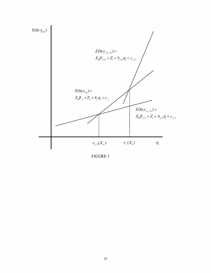
E(ln y ijt) =

Xitβ j +Z i + bjη i +c j

E(ln yi, j −1,t) =

Xitβ j −1 + Zi + bj−1ηi + c j −1

E(ln y i,j + 1,t ) =

Xitβ j +1 + Zi + bj +1ηi + c j +1

E(ln yijt )

η iv j −1(X it ) v j (Xit )

FIGURE 1

35

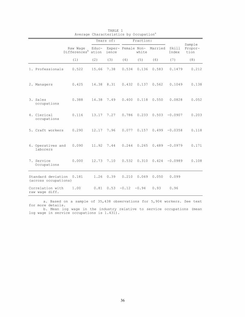
TABLE 1 Average Characteristics by Occupationa

Years of: Fraction: ───────────── ──────────────────── Sample Raw Wage Educ- Exper- Female Non- Married Skill Propor- Differencesb ation ience white Index tion (1) (2) (3) (4) (5) (6) (7) (8)

1. Professionals 0.522 15.66 7.38 0.534 0.136 0.583 0.1479 0.212 2. Managers 0.425 14.38 8.31 0.432 0.137 0.562 0.1049 0.138 3. Sales 0.388 14.38 7.49 0.400 0.118 0.550 0.0828 0.052 occupations 4. Clerical 0.116 13.17 7.27 0.786 0.233 0.503 -0.0907 0.203 occupations 5. Craft workers 0.290 12.17 7.96 0.077 0.157 0.499 -0.0358 0.118 6. Operatives and 0.090 11.92 7.44 0.244 0.265 0.489 -0.0979 0.171 laborers 7. Service 0.000 12.73 7.10 0.532 0.310 0.424 -0.0989 0.108 Occupations Standard deviation 0.181 1.26 0.39 0.210 0.069 0.050 0.099 (across occupations) Correlation with 1.00 0.81 0.53 -0.12 -0.94 0.93 0.96 raw wage diff.

a. Based on a sample of 35,438 observations for 5,904 workers. See text for more details. b. Mean log wage in the industry relative to service occupations (mean log wage in service occupations is 1.431).

36

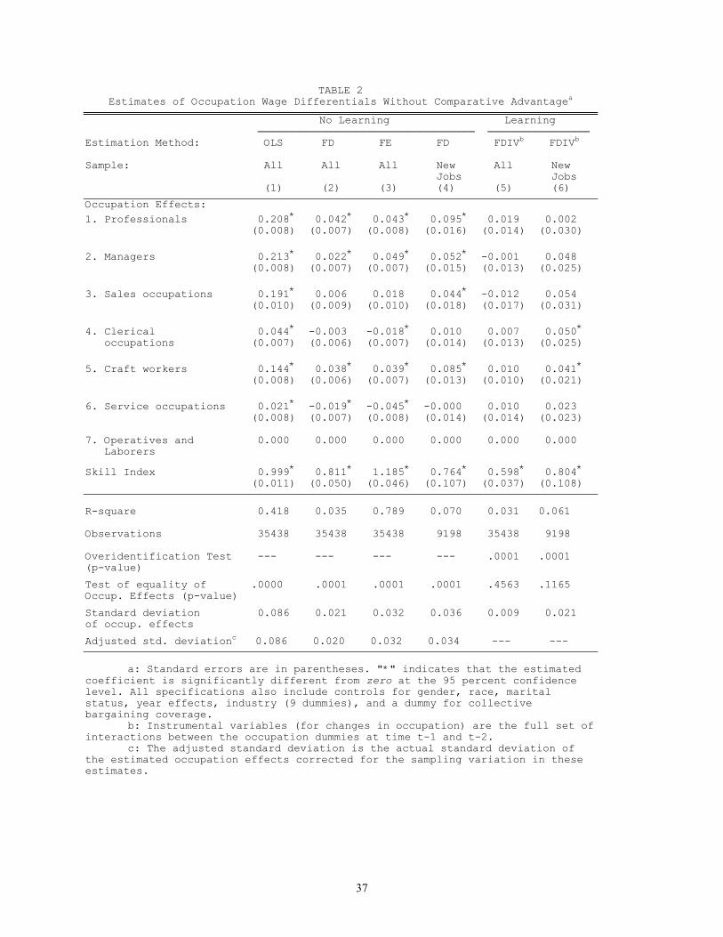
TABLE 2 Estimates of Occupation Wage Differentials Without Comparative Advantagea

No Learning Learning ────────────────────────────────── ──────────────── Estimation Method: OLS FD FE FD FDIVb FDIVb

Sample: All All All New All New Jobs Jobs (1) (2) (3) (4) (5) (6)

Occupation Effects: 1. Professionals 0.208* 0.042* 0.043* 0.095* 0.019 0.002 (0.008) (0.007) (0.008) (0.016) (0.014) (0.030) 2. Managers 0.213* 0.022* 0.049* 0.052* -0.001 0.048 (0.008) (0.007) (0.007) (0.015) (0.013) (0.025) 3. Sales occupations 0.191* 0.006 0.018 0.044* -0.012 0.054 (0.010) (0.009) (0.010) (0.018) (0.017) (0.031) 4. Clerical 0.044* -0.003 -0.018* 0.010 0.007 0.050* occupations (0.007) (0.006) (0.007) (0.014) (0.013) (0.025) 5. Craft workers 0.144* 0.038* 0.039* 0.085* 0.010 0.041* (0.008) (0.006) (0.007) (0.013) (0.010) (0.021) 6. Service occupations 0.021* -0.019* -0.045* -0.000 0.010 0.023 (0.008) (0.007) (0.008) (0.014) (0.014) (0.023) 7. Operatives and 0.000 0.000 0.000 0.000 0.000 0.000 Laborers

Skill Index 0.999* 0.811* 1.185* 0.764* 0.598* 0.804* (0.011) (0.050) (0.046) (0.107) (0.037) (0.108)

R-square 0.418 0.035 0.789 0.070 0.031 0.061 Observations 35438 35438 35438 9198 35438 9198 Overidentification Test --- --- --- --- .0001 .0001 (p-value)

Test of equality of .0000 .0001 .0001 .0001 .4563 .1165 Occup. Effects (p-value)

Standard deviation 0.086 0.021 0.032 0.036 0.009 0.021 of occup. effects

Adjusted std. deviationc 0.086 0.020 0.032 0.034 --- ---

a: Standard errors are in parentheses. "*" indicates that the estimated coefficient is significantly different from zero at the 95 percent confidence level. All specifications also include controls for gender, race, marital status, year effects, industry (9 dummies), and a dummy for collective bargaining coverage. b: Instrumental variables (for changes in occupation) are the full set of interactions between the occupation dummies at time t-1 and t-2. c: The adjusted standard deviation is the actual standard deviation of the estimated occupation effects corrected for the sampling variation in these estimates.

37

TABLE 3 Estimates of Occupation Wage Differentials With Comparative Advantagea

No Learning Learning ────────────────────────────────── ──────────────── Estimation Method: OLS NLIV NLIV Sample: All All All ─────────────── ─────────────── ─────────────── Occupation effects: Main Interactedb Main Interactedb Main Interactedb

(1) (2) (3) (4) (5) (6)

1. Professionals 0.263* 1.120* 0.069 1.271* 0.029 1.259* (0.008) (0.034) (0.034) (0.086) (0.049) (0.116) 2. Managers 0.233* 1.332* 0.046 1.201* 0.032 1.196 (0.008) (0.036) (0.034) (0.077) (0.049) (0.110) 3. Sales occupations 0.199* 1.476* 0.054 1.218* 0.087 1.224 (0.011) (0.047) (0.038) (0.083) (0.061) (0.128) 4. Clerical 0.066* 1.027 0.033 1.162* 0.004 1.099 occupations (0.008) (0.036) (0.031) (0.073) (0.044) (0.097) 5. Craft workers 0.168* 1.138* 0.040 1.023 -0.024 0.971 (0.008) (0.044) (0.026) (0.065) (0.036) (0.086) 6. Service occupations -0.037* 1.107* 0.047 1.127 0.088 1.204 (0.009) (0.042) (0.035) (0.076) (0.060) (0.133) 7. Operatives and 0.000 1.000 0.000 1.000 0.000 1.000 Laborers

Proportionality factorb --- 0.8652* 0.7847* between measured and (0.0710) (0.0899) unmeasured skills

Endogenous Variablesc --- w1 w1,D0

Instrumental Variablesc --- D0*D1 D1*D2,SK*D2,E*D2

Observations 35438 35438 35438

Overidentification test --- .0000 .0000 (p-value) Test of equality of .0000 .4372 .2807 Occupation Effects (p-value) Test of equality of .0000 .0357 .0852 Interaction slopes (p-value) Test of proportionalityb --- .1391 .5403 (p-value) Standard deviation 0.096 0.020 0.040 of occupation effects Adjusted std. Deviationd 0.095 --- ---

38

Notes to Table 3 a: Standard errors are in parentheses. In the case of main effects, "*" indicates that the estimated coefficient is significantly different from zero at the 95 percent confidence level. In the case of interactions, "*" indicates that the estimated coefficient is significantly different from one at the 95 percent confidence level. All specifications also include controls for gender, race, marital status, year effects, industry (9 dummies), collective bargaining coverage, and (except in columns 1-2) occupation-specific experience effects. b: In columns 1-2, the interaction terms indicate the effect of measured skills in the occupation relative to operatives and laborers (effect normalized to 1 in service occupations). In columns 3-6, the interaction terms indicate the effect of both measured and unmeasured skills in the occupation, again relative to operatives and laborers, but these occupation-specific slopes for measured and unmeasured skills are constrained to have the same proportionality factor across all occupations. The estimated proportionality factor is reported at the bottom of the first panel; the test of the proportionality restriction is reported in the second panel. c: In the endogenous variables, w1 stands for the lagged wage and D0 stands for contemporaneous values of the occupation dummies {Dijt, j=1,..,6}. In the instrumental variables, D1 and D2 stand for the first and second lag of occupations dummies, SK stands for the skill index, and E stands for experience. d: The adjusted standard deviation is the actual standard deviation of the estimated occupation effects corrected for the sampling variation in these estimates.

39

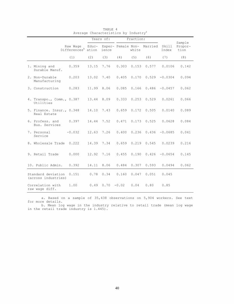
TABLE 4 Average Characteristics by Industrya

Years of: Fraction: ───────────── ──────────────────── Sample Raw Wage Educ- Exper- Female Non- Married Skill Propor- Differencesb ation ience white Index tion (1) (2) (3) (4) (5) (6) (7) (8)

1. Mining and 0.359 13.15 7.76 0.303 0.153 0.577 0.0106 0.142 Durable Manuf. 2. Non-Durable 0.203 13.02 7.40 0.405 0.170 0.529 -0.0304 0.094 Manufacturing 3. Construction 0.283 11.99 8.06 0.085 0.166 0.486 -0.0457 0.062 4. Transpo., Comm., 0.387 13.44 8.09 0.333 0.253 0.529 0.0261 0.066 Utilities 5. Finance. Insur., 0.348 14.10 7.43 0.659 0.172 0.505 0.0140 0.089 Real Estate 6. Profess. and 0.397 14.44 7.52 0.471 0.173 0.525 0.0628 0.084 Bus. Services 7. Personal -0.032 12.63 7.26 0.400 0.236 0.436 -0.0685 0.041 Service 8. Wholesale Trade 0.222 14.39 7.34 0.659 0.219 0.545 0.0239 0.216 9. Retail Trade 0.000 12.92 7.16 0.455 0.190 0.426 -0.0654 0.145 10. Public Admin. 0.392 14.11 8.06 0.484 0.307 0.593 0.0494 0.062

Standard deviation 0.151 0.78 0.34 0.160 0.047 0.051 0.045 (across industries) Correlation with 1.00 0.49 0.70 -0.02 0.04 0.80 0.85 raw wage diff.

a. Based on a sample of 35,438 observations on 5,904 workers. See text

for more details. b. Mean log wage in the industry relative to retail trade (mean log wage

in the retail trade industry is 1.445).

40

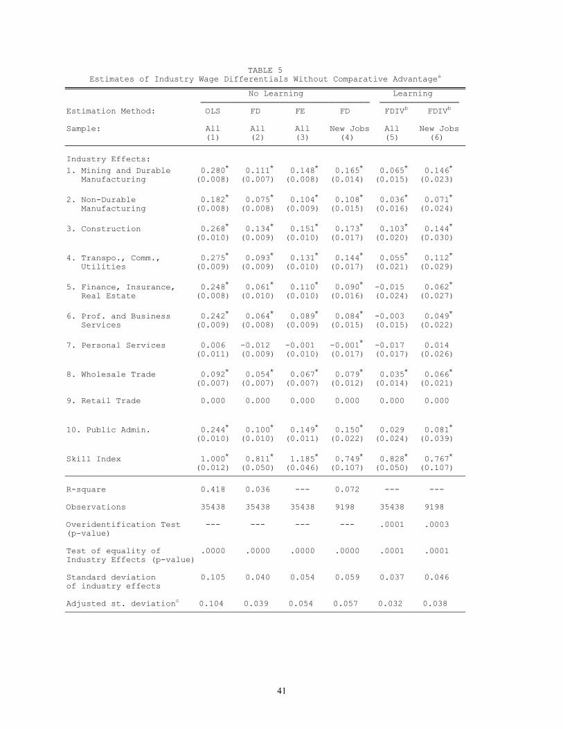
TABLE 5 Estimates of Industry Wage Differentials Without Comparative Advantagea

No Learning Learning ────────────────────────────────── ──────────────── Estimation Method: OLS FD FE FD FDIVb FDIVb

Sample: All All All New Jobs All New Jobs (1) (2) (3) (4) (5) (6)

Industry Effects: 1. Mining and Durable 0.280* 0.111* 0.148* 0.165* 0.065* 0.146* Manufacturing (0.008) (0.007) (0.008) (0.014) (0.015) (0.023) 2. Non-Durable 0.182* 0.075* 0.104* 0.108* 0.036* 0.071* Manufacturing (0.008) (0.008) (0.009) (0.015) (0.016) (0.024) 3. Construction 0.268* 0.134* 0.151* 0.173* 0.103* 0.144* (0.010) (0.009) (0.010) (0.017) (0.020) (0.030) 4. Transpo., Comm., 0.275* 0.093* 0.131* 0.144* 0.055* 0.112* Utilities (0.009) (0.009) (0.010) (0.017) (0.021) (0.029) 5. Finance, Insurance, 0.248* 0.061* 0.110* 0.090* -0.015 0.062* Real Estate (0.008) (0.010) (0.010) (0.016) (0.024) (0.027) 6. Prof. and Business 0.242* 0.064* 0.089* 0.084* -0.003 0.049* Services (0.009) (0.008) (0.009) (0.015) (0.015) (0.022) 7. Personal Services 0.006 -0.012 -0.001 -0.001* -0.017 0.014 (0.011) (0.009) (0.010) (0.017) (0.017) (0.026) 8. Wholesale Trade 0.092* 0.054* 0.067* 0.079* 0.035* 0.066* (0.007) (0.007) (0.007) (0.012) (0.014) (0.021) 9. Retail Trade 0.000 0.000 0.000 0.000 0.000 0.000 10. Public Admin. 0.244* 0.100* 0.149* 0.150* 0.029 0.081* (0.010) (0.010) (0.011) (0.022) (0.024) (0.039) Skill Index 1.000* 0.811* 1.185* 0.749* 0.828* 0.767* (0.012) (0.050) (0.046) (0.107) (0.050) (0.107)

R-square 0.418 0.036 --- 0.072 --- --- Observations 35438 35438 35438 9198 35438 9198 Overidentification Test --- --- --- --- .0001 .0003 (p-value) Test of equality of .0000 .0000 .0000 .0000 .0001 .0001 Industry Effects (p-value) Standard deviation 0.105 0.040 0.054 0.059 0.037 0.046 of industry effects Adjusted st. deviationc 0.104 0.039 0.054 0.057 0.032 0.038

41

Notes to Table 5 a: Standard errors are in parentheses. “*” indicates that the estimated coefficient is significantly different from zero at the 95 percent confidence level. All specifications also include controls for gender, race, marital status, year effects, occupation (6 dummies), and collective bargaining coverage.

b: Instrumental variables (for changes in industry affiliation) are the full set of interactions between the industry affiliation dummies at time t-1 and t-2. c: The adjusted standard deviation is the actual standard deviation of the estimated industry effects corrected for the sampling variation in these estimates.

42

TABLE 6 Estimates of Inter-Industry Wage Differentials With Comparative Advantagea

No Learning Learning ────────────────────────────────────────────────── ──────────────────────────────── Estimation Method: OLS NLIV NLIV NLIV NLIV Sample: All All New Jobs All New Jobs ─────────────── ─────────────── ─────────────── ─────────────── ─────────────── Industry effects: Main Interactedb Main Interactedb Main Interactedb Main Interactedb Main Interactedb (1) (2) (3) (4) (5) (6) (7) (8) (9) (10)

1. Mining and Durable 0.282* 1.182

* 0.163

* 1.124* 0.254

* 1.138 0.144* 1.158 0.182* 0.978

Manufacturing (0.008) (0.042) (0.033) (0.062) (0.051) (0.100) (0.047) (0.100) (0.060) (0.119)

2. Non-Durable 0.187* 1.208* 0.093

* 1.089 0.123* 1.114 0.112* 1.144 0.167* 1.282

Manufacturing (0.009) (0.046) (0.033) (0.060) (0.051) (0.096) (0.049) (0.100) (0.089) (0.179) 3. Construction 0.248* 0.823* 0.124* 1.005 0.173* 0.968 0.146* 1.115 0.169* 0.875 (0.011) (0.054) (0.040) (0.087) (0.056) (0.133) (0.065) (0.152) (0.069) (0.147) 4. Transpo., Comm., 0.276* 0.969 0.114* 1.094 0.201* 1.182 0.053 1.275 0.190* 1.223 Utilities (0.009) (0.048) (0.041) (0.079) (0.069) (0.135) (0.063) (0.156) (0.097) (0.201) 5. Finance, Insurance, 0.237* 1.296* 0.037 1.212* 0.125* 1.362* -0.040 1.156 0.029 1.241 Real Estate (0.009) (0.049) (0.040) (0.081) (0.061) (0.131) (0.052) (0.137) (0.072) (0.181) 6. Prof. and Business 0.224* 1.341* 0.052 1.176* 0.092 1.223* 0.028 1.132 0.084 1.098 Services (0.009) (0.049) (0.036) (0.070) (0.052) (0.108) (0.046) (0.105) (0.062) (0.133) 7. Personal Services -0.023 0.625* -0.050 0.970 -0.047 0.939 0.066 1.232 0.112 1.167 (0.012) (0.056) (0.054) (0.123) (0.078) (0.192) (0.105) (0.232) (0.145) (0.311) 8. Wholesale Trade 0.102* 0.877* 0.069 1.148* 0.109* 1.165 0.095 1.248* 0.180* 1.219 (0.007) (0.032) (0.033) (0.069) (0.051) (0.108) (0.051) (0.118) (0.080) (0.166)

43

9. Retail Trade 0.000 1.000 0.000 1.000 0.000 1.000 0.000 1.000 0.000 1.000 --- --- --- --- --- --- --- --- --- ---

10. Public 0.251* 0.936 0.119* 1.155* 0.183* 1.233 0.099 1.300 0.039 1.119

Administration (0.010) (0.047) (0.036) (0.078) (0.064) (0.162) (0.061) (0.176) (0.077) (0.195)

Proportionalityb --- 0.987* 0.724

* 0.860

* 0.671

*

Parameter (0.063) (0.103) (0.077) (0.111)

Endogenous Variables --- w1 w1 w1,D0 w1,D0 Instrumental Variablesc --- D0*D1 D0*D1 D1*D2,SK*D2,E*D2 D1*D2,SK*D2,E*D2 Observations 35438 35428 9198 35438 9198 Overidentification test --- .0001 .0002 .0000 .0169 (p-value) Test of equality of .0000 .0000 .0000 .0018 .0259 Industry Effects (p-value) Test of equality of .0000 .1331 .2473 .6980 .1996 Industry Slopes (p-value) Standard deviation 0.099 0.061 0.086 0.058 0.038 of industry effects Adjusted st. deviationd 0.098 0.048 0.065 --- --- Test of proportionalityb --- .9645 .4487 .4649 .5597 (p-value)

a: In the case of main effects, “*” indicates that the estimated coefficient is significantly different from zero at the 95 percent confidence level. In the case of interactions, “*” indicates that the estimated coefficient is significantly different from one at the 95 percent confidence level. All specifications also include controls for gender, race, marital status, year effects, occupation (6 dummies), collective bargaining coverage, and industry-specific experience effects (except in the model of columns 1-2). b: In columns 1-2, the interaction terms indicate the effect of measured skills in the industry relative to retail trade (effect normalized to 1 in this industry). In columns 3-10, the interaction terms indicate the effect of both measured and unmeasured skills in the industry, again relative to retail trade, but these industry-specific slopes for measured and unmeasured skills are constrained to be proportional across all industries. The estimated constant of proportionality between measured and unmeasured skills is reported at the bottom of the first panel; the test of the proportionality restriction is reported in the second panel.

44

c: In the endogenous variables, w1 stands for the lagged wage and D0 stands for contemporaneous values of the occupation dummies {Dijt, j=1,..,6}. In the instrumental variables, D1 and D2 stand for the first and second lag of occupations dummies, SK stands for the skill index, and E stands for experience.

d. The adjusted standard deviation is the actual standard deviation of the estimated industry effects corrected for the sampling variation in these estimates.

45

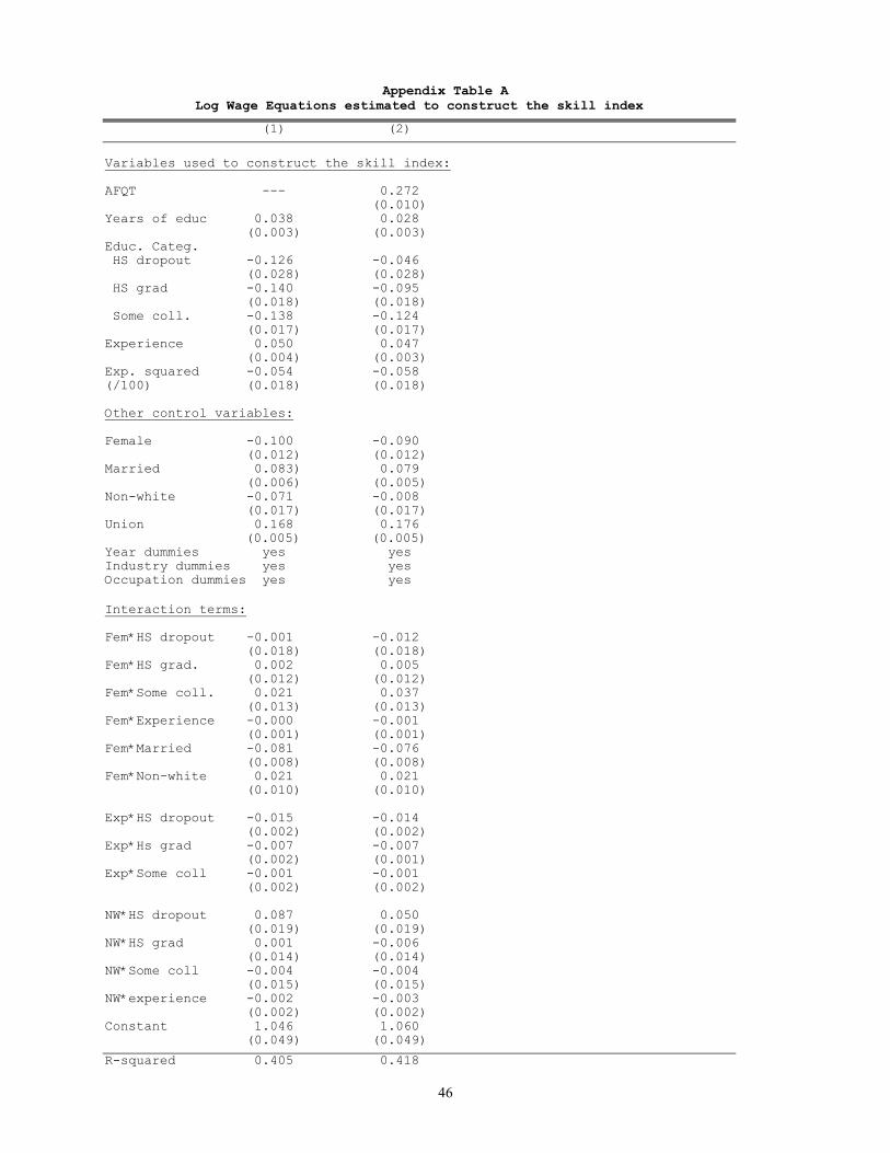
Appendix Table A Log Wage Equations estimated to construct the skill index

(1) (2)

Variables used to construct the skill index: AFQT --- 0.272 (0.010) Years of educ 0.038 0.028 (0.003) (0.003) Educ. Categ. HS dropout -0.126 -0.046 (0.028) (0.028) HS grad -0.140 -0.095 (0.018) (0.018) Some coll. -0.138 -0.124 (0.017) (0.017) Experience 0.050 0.047 (0.004) (0.003) Exp. squared -0.054 -0.058 (/100) (0.018) (0.018) Other control variables: Female -0.100 -0.090 (0.012) (0.012) Married 0.083) 0.079 (0.006) (0.005) Non-white -0.071 -0.008 (0.017) (0.017) Union 0.168 0.176

(0.005) (0.005) Year dummies yes yes Industry dummies yes yes Occupation dummies yes yes Interaction terms: Fem*HS dropout -0.001 -0.012 (0.018) (0.018) Fem*HS grad. 0.002 0.005 (0.012) (0.012) Fem*Some coll. 0.021 0.037 (0.013) (0.013) Fem*Experience -0.000 -0.001 (0.001) (0.001) Fem*Married -0.081 -0.076 (0.008) (0.008) Fem*Non-white 0.021 0.021 (0.010) (0.010) Exp*HS dropout -0.015 -0.014 (0.002) (0.002) Exp*Hs grad -0.007 -0.007 (0.002) (0.001) Exp*Some coll -0.001 -0.001 (0.002) (0.002) NW*HS dropout 0.087 0.050 (0.019) (0.019) NW*HS grad 0.001 -0.006 (0.014) (0.014) NW*Some coll -0.004 -0.004 (0.015) (0.015) NW*experience -0.002 -0.003 (0.002) (0.002) Constant 1.046 1.060 (0.049) (0.049)

R-squared 0.405 0.418

46

Note: All models are estimated on a sample of 35,438 observations for 5,904 workers. The skill index is constructed by computing a predicted wage from equation (2) using only the variables AFQT, education (both years of education and education categories) and experience, and holding the other variables (female, married, non-white, union, year, industry and occupation) at their average sample values.

47

Appendix B: Choice of instruments This appendix explains the choice of the interaction between the sector affiliation at time t-1 and t-2 as the main set of instruments in model with comparative advantage and learning. The intuition for this choice is most easily understood using of Figure 1. First note that in the most general model with comparative advantage and learning, Figure 1 remains as is except that the unmeasured ability ηi is replaced by its expected value conditional on the available information, mi,t-1. Consider the case of sectors j and j-1 in the Figure 1. There are four possible “sector histories” in these two sectors. Workers can either “stay” in sector j-1 or j in both time periods, or switch (from j to j-1 or from j-1 to j). Workers with expected ability close to the critical value vj-1(X) are more likely to switch sector than either workers with expected ability clearly lower than vj-1(X) (sector j-1 stayers) or clearly higher than vj-1(X) (sector j-1 stayers). In terms of expected ability and wages, “switchers” currently in sector j-1 should earn more than other workers in sector j-1, while “switchers” currently in sector j should earn less than other workers in sector j. Appendix Tables B1 (occupations) and B2 (industries) show that the data is broadly consistent with this prediction. These tables show the average log wages as a function of current and previous sector affiliations. For example, consider operatives and laborers as sector j-1 and craft workers as sector j. As expected, “stayers” in the craft occupation earn more (0.08) than craft workers who switched from operatives and laborers to craft (-0.09). By contrast, workers who “switch down” from craft to operatives and laborers earn more (-0.11) than “stayers” in the operative and laborers occupation (-0.17). This example shows how the interaction between sector affiliation at time t and t-1 helps predict wages even after controlling for the current sector affiliation. Similar reasoning can be used to show how the interaction between sector affiliation at time t-1 and t-2 can be used to predict sector affiliation at time t. Recall that like the lagged wage, the current sector affiliation is endogenous in the model with comparative advantage and learning. Consider, for example, the choice of sector at time t of individuals observed to be in sector j at time t-1. Remember from Figure 1 that the expected ability of sector j workers (at time t-1) who were in sector j-1 at time t-2 should be lower (close to vj-1(X)) than the expected ability of sector j workers who were also in sector j at time t-2. Consider a positive productivity signal that increases expected ability mi . Since sector j stayers (at time t-1 and t-2) are closer to the upper critical value vj(X) than the switchers who just came from sector j-1, the stayers are more likely to move to sector j+1 at time t than the switchers. This shows how the interaction between sector affiliation at time t-1 and t-2 can be used to predict sector affiliation at time t. In summary, sector histories (interaction between sector dummies at time t-1 and t-2) should help predict both the wage at t-1 and the sector affiliation at time t in the model with comparative advantage and learning. Appendix Tables B1 and B2 suggest they do so in the case of the wage. A more formal test consists of testing the predictive power of the sector histories on the lagged wage and current affiliation after controlling for all other exogenous variables of the model. In a linear model, this test is just the standard F-test of the predictive power of the excluded instruments in the first-stage equation. Testing for the predictive power of instruments is more complicated in a non-linear context. In the linear model y = xβ + e, the “first-stage” consists of projecting all the right hand side variables (x) on the set of instruments, where the x variables also happen to be (minus) the derivative (or gradient) of e with respect the parameters β (since e = y - xβ). In the non-linear model, the equivalent of the first-stage is thus a regression of the gradient of e with respect to the structural parameters. Those derivatives will typically be non-linear combinations of various x variables. One way to measure the predictive power of the instruments is thus to compute F-tests on the excluded instruments in these “gradient” regressions. The more intuitive approach we follow is to linearize the gradients as a function of the various explanatory variables. Once this linearization is performed, we can simply compute the usual F-test on the “first-stage” equations for the lagged wage and the current sector affiliation. To be consistent with the estimated models of Table 3 and Table 6, our excluded instruments are the interactions between sector affiliation at time t-1 and t-2 as well as interactions of sector affiliation at time t-2 with the skill index and experience. The F-statistics are reported below. In all cases, they largely exceed the critical values (at the 95 percent confident level) of 1.26 for industries and 1.39 for occupations:

48

F-test of the predictive power of instruments Lagged Current sector # of excluded

wage (range of values) instruments Occupations: 16.27 16.27-38.69 60 Industries: 11.46 17.45-26.68 117 As mentioned in the text and tables, in the case with comparative advantage but no learning we use the sector affiliations at time t and t-1 (instead of t-1 and t-2) as instruments. In this case, the F-statistics are 10.70 and 8.27 for occupations and industries, respectively, which largely exceeds the critical values. Overidentification test Having established that the instruments predict well the lagged wage and sector affiliation, it is also important to know whether the instruments are valid in the sense that they are uncorrelated with the error term in equation (13). As discussed in Section 2.4, the overidentification test is the natural way of testing this hypothesis. In a complicated non-linear model like ours, however, this test is an omnibus test that can fail either because the model is misspecified or because the model is well-specified but the instruments are invalid. Intuitively speaking, the model is overidentified when there are more instruments than parameters. So the model may either fail the overidentification test because not enough parameters are included (model misspecified) or because some of the instruments are invalid. In the absence of further information, we cannot conclude that the instruments are invalid just because our models do not generally pass the overidenfication test. For example, we use throughout the paper a convenient single-index model in which wages in all sectors are linear functions of the same underlying index of measured and unmeasured skills. While this assumption is used for reasons of convenience and clarity, it is well-known to be restrictive in models with more than two sectors (see Heckman and Scheinkman, 1987). By contrast, Lemieux (1998) argues that the single index model imposes little restriction when only two sectors are used. It is easy to see in the three sector case illustrated in Figure 1 why the single index model is restrictive. Consider sector j-1 and j. The relative slope and intercepts in the two sectors can be estimated using the subsample of workers that are in these two sectors at time t and t-1 (and t-2 in the model with learning). Similarly, observations from sectors j and j+1 can be used to estimate the relative slope and intercepts in these two sectors. Say we normalize the slope in sector j-1 to 1 and estimate the slope of sector j relative to j-1 to be 1.2. If the slope in sector j+1 relative to j is also 1.2, it follows that the slope of sector j+1 relative to j-1 is 1.44. According to the model, it is unlikely that a worker would switch directly from sector j-1 to j+1 or vice versa. But since those transitions are actually observed in the data, it is possible to use the subsample of workers in the two sectors in two consecutive periods to estimate the relative slope and intercepts in sectors j-1 and j+1. To the extent that the resulting slope (for example) is statistically different from 1.44, the overidentification test will fail since different identification strategies yield different estimates of the slopes. In this case we would conclude, however, that the failure of the overidentification is a consequence of the fact that the single index model is an oversimplication. In light of this example, we re-estimate the model of columns 3 and 4 of Table 3 using only workers who either stay in the same occupation at t and t-1 (66 percent of the sample) or move across adjoining occupations according to the ranking used in the tables (14 percent of the sample).24 Consistent with our expectations, the p-value on the overidentification test moves from 0.0000 (Table 3) to 0.2776. In other words, the overidentification restrictions can no longer be rejected at standard significance levels.

24 Note that except for clerical and service occupations, occupational mobility tends to be concentrated between adjoining sectors. There is a total of 11969 occupation transitions (34 percent of all observations) in the data. Of those 4789 are between “adjoining” occupation (i.e. between occupation 1 (professionals) and 2 (managers), 2 and 3 (sales), etc.). Of the 7180 transitions among “non-adjoining” occupations, 5316 involve either clerical or service occupations. This pattern of transitions among occupations suggests that these two particular occupations are difficult to rank in terms of an occupational hierarchy based on a single index of skills. 49

Another possible source of misspecification is that, as mentioned in Section 2, we assume throughout the paper that this period's wage is specified before production occurs. This, in essence, assumes away the presence of piece rate contracts or of any form of contracts where the level of pay is determined ex post, such as contracts where part of the compensation is based on a subjective evaluation of performance. One consequence of having some workers in our sample being paid piece rates or commissions would thus be to affect the validity of our overidentifying restrictions. To explore whether this might be one reason why the restrictions are all rejected, we re-estimated our occupation models by first restricting the sample to workers who were in occupations in which the percentage of piece rate workers is below 10%. To impose this sample selection restriction, we looked at the percentage of workers in the sample who are paid commissions or piece rates between 1988 and 1990, the three years in which this information is available in the NLSY. We then exclude from our total sample observations that belong to one of the 3-digit occupations where piece rates account for at least 10% of the observations between 1988 and 1990.25 As it turns out, the overidentifying restrictions are still decidedly rejected, although the p-value does increase somewhat to 0.0003 for the model with comparative advantage only.26 There is hardly any change for the model with both learning and comparative advantage. If we further restrict the sample to occupations where piece rates account for less than 5% of the sample (this reduces the sample size to 18,108 observations), we basically get the same results as in the previous paragraph for the full sample: the overidentifying restrictions are rejected in both models. For the subsample of new jobs only, though, both models pass the test, with a p-value of 0.2185 for the comparative advantage model and 0.0827 for the model. In summary, our assumptions that wages are paid in advance and depend on a single index of skill are restrictive and clearly contribute to the rejection of the overidentification restrictions of the model. It would be useful to enrich the empirical model in future research to accommodate departures from these assumptions. But despite the limitations of our approach, we think our model and instrumentation strategy are a useful way of analyzing the role of comparative advantage and learning in sectoral wage determination.

25This reduces the sample size from to 24,726 observations. Not surprisingly, the main deletions are made in sales-related occupations, where we are more likely to find workers paid commissions, and also among operatives, which account for the bulk of piece rate workers. A list of all deleted 3-digit occupations is available upon request. 26The improvement is more substantial if we look at new jobs. In fact, we cannot reject the restrictions (p-value=0.0904) for the model with comparative advantage. The restrictions are still rejected for the full model with learning and comparative advantage (p-value=0.0175).

50

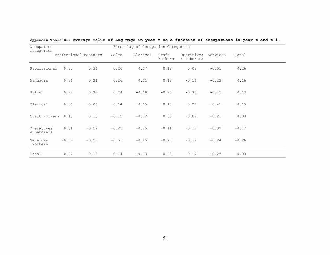
Appendix Table B1: Average Value of Log Wage in year t as a function of occupations in year t and t-1.

Occupation First lag of Occupation Categories Categories Professional Managers Sales Clerical Craft Operatives Services Total Workers & laborers

Professional 0.30 0.36 0.26 0.07 0.18 0.02 -0.05 0.26 Managers 0.36 0.21 0.26 0.01 0.12 -0.16 -0.22 0.16 Sales 0.23 0.22 0.24 -0.09 -0.20 -0.35 -0.45 0.13 Clerical 0.05 -0.05 -0.14 -0.15 -0.10 -0.27 -0.41 -0.15 Craft workers 0.15 0.13 -0.12 -0.12 0.08 -0.09 -0.21 0.03 Operatives 0.01 -0.22 -0.25 -0.25 -0.11 -0.17 -0.39 -0.17 & Laborers Services -0.06 -0.26 -0.51 -0.45 -0.27 -0.39 -0.24 -0.26 workers

Total 0.27 0.16 0.14 -0.13 0.03 -0.17 -0.25 0.00

51

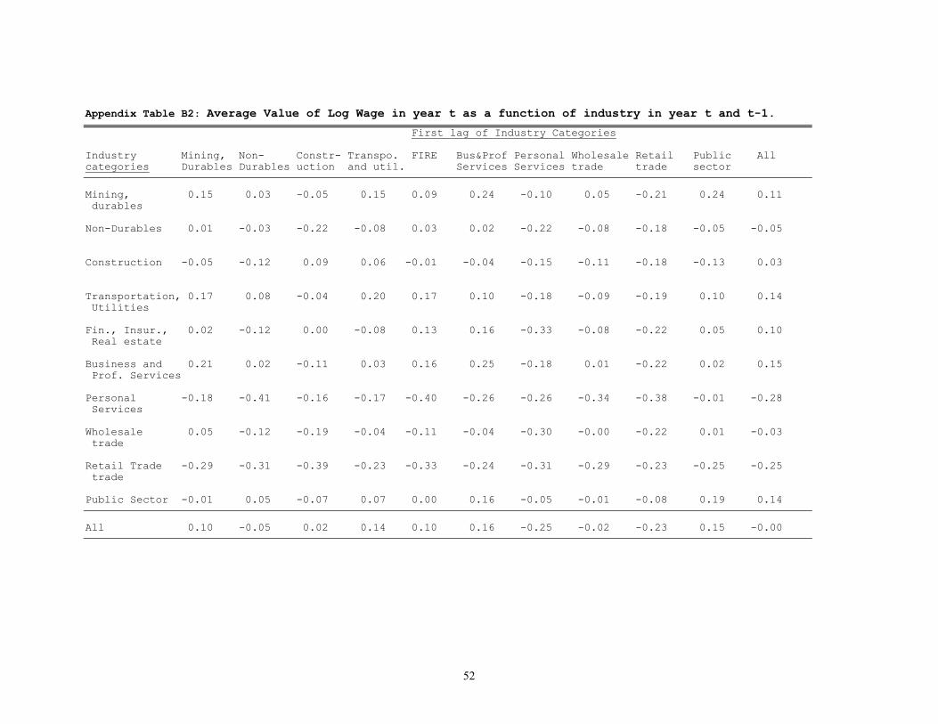
52

Appendix Table B2: Average Value of Log Wage in year t as a function of industry in year t and t-1.

First lag of Industry Categories Industry Mining, Non- Constr- Transpo. FIRE Bus&Prof Personal Wholesale Retail Public All categories Durables Durables uction and util. Services Services trade trade sector

Mining, 0.15 0.03 -0.05 0.15 0.09 0.24 -0.10 0.05 -0.21 0.24 0.11 durables Non-Durables 0.01 -0.03 -0.22 -0.08 0.03 0.02 -0.22 -0.08 -0.18 -0.05 -0.05 Construction -0.05 -0.12 0.09 0.06 -0.01 -0.04 -0.15 -0.11 -0.18 -0.13 0.03 Transportation, 0.17 0.08 -0.04 0.20 0.17 0.10 -0.18 -0.09 -0.19 0.10 0.14 Utilities Fin., Insur., 0.02 -0.12 0.00 -0.08 0.13 0.16 -0.33 -0.08 -0.22 0.05 0.10 Real estate Business and 0.21 0.02 -0.11 0.03 0.16 0.25 -0.18 0.01 -0.22 0.02 0.15 Prof. Services Personal -0.18 -0.41 -0.16 -0.17 -0.40 -0.26 -0.26 -0.34 -0.38 -0.01 -0.28 Services Wholesale 0.05 -0.12 -0.19 -0.04 -0.11 -0.04 -0.30 -0.00 -0.22 0.01 -0.03 trade Retail Trade -0.29 -0.31 -0.39 -0.23 -0.33 -0.24 -0.31 -0.29 -0.23 -0.25 -0.25 trade Public Sector -0.01 0.05 -0.07 0.07 0.00 0.16 -0.05 -0.01 -0.08 0.19 0.14

All 0.10 -0.05 0.02 0.14 0.10 0.16 -0.25 -0.02 -0.23 0.15 -0.00