1

Learning by Collaborative and Individual-Based Recommendation Agents

Dan Ariely, Sloan School of Management, MITJohn G. Lynch, Jr., Fuqua School of Business, Duke University

Manuel Aparicio IV, Saffron Technology, Inc.

RUNNING HEAD: Learning by Recommendation Agents

2

Learning by Collaborative and Individual-Based Recommendation Agents

ABSTRACT

Intelligent recommendation systems can be based on two basic principles: collaborative filters

and individual-based agents. In this work we examine the learning function that results from these two

general types of learning smart agents. There has been significant work on the predictive properties of

each type, but no work has examined the patterns in their learning from feedback over repeated trials.

Using simulations, we create clusters of “consumers” with heterogeneous utility functions and errorful

reservation utility thresholds. The consumers go shopping with one of the designated smart agents –

receive recommendations from the agents, and purchase products they like and reject ones they do not.

Based on the purchase / no purchase behavior of the consumers, agents learn about the consumers and

potentially improve the quality of their recommendations. We characterize learning curves by

modified exponential functions with an intercept for percent of recommendations accepted at trial 0, an

asymptotic rate of recommendation acceptance, and a rate at which learning moves from intercept to

asymptote. We compare the learning of a baseline random recommendation agent, an individual-based

logistic-regression agent, and two types of collaborative filters that rely on K-mean clustering (popular

in most commercial applications) and nearest-neighbor algorithms. Compared to the collaborative

filtering agents, the individual agent: 1) learns slower initially, but performs better in the long run

when the environment is stable; 2) is less negatively affected by permanent changes in the consumer’s

utility function; 3) is less adversely affected by error in the reservation threshold to which consumers

compare a recommended product’s utility. The K-mean agent reaches a lower asymptote but

approaches it faster, reflecting a surprising stickiness of target classifications after feedback from

recommendations made under initial (incorrect) hypotheses.

3

The emergence of Internet retailing provides consumers with an explosion of products available

at greatly reduced search costs. Alba et al. (1997) argued that this is of little benefit to consumers

without an efficient way to screen products effectively. Without such screening, consumers may suffer

from information overload (Jacoby, Speller, and Berning 1974) or stop searching long before

exhausting the set of relevant products (Diehl, Kornish, and Lynch, in press).

To overcome this inherent difficulty, smart recommendation agents have emerged (Ansari,

Essegaier, and Kohli 2000; Iacobucci, Arabie, and Bodapati 2000, Schafer, Konstan, and Riedl 1999;

Shardanand and Maes 1995; West et al. 1999). Smart agents counteract the information explosion

problem by “considering” a large number of alternatives and recommending only a small number to

the consumer, very much like a salesperson who is highly knowledgeable about both the alternatives

available and the consumer’s tastes. An effective screening mechanism allows consumers to expend

processing effort only for those few recommended alternatives that are actively inspected. If the

agent’s screening rule is highly correlated with consumers’ overall preferences, consumers’ best choice

from this small set will have utility almost as high as that if every alternative in the universe were

inspected – but with dramatically reduced effort on their part (Häubl and Trifts 2000).

Our aim in the current research is to describe the properties of two broad classes of intelligent

agents that have received significant attention in academic research and commercial applications.

Much work has evaluated agents’ accuracy at a given point in time, but none, to our knowledge,

examines the differences in their patterns of learning from feedback over trials. We build simulations

of these agents and explore the antecedents of learning patterns of each type.

TWO TYPES OF AGENTS: COLLABORATIVE FILTERING VS. INDIVIDUAL MODELS

While there are many different interpretations of the term “intelligent agents,” our focus here is

4

intelligent “recommendation agents” that learn customers’ preferences by observing their actions, and

use this feedback to improve recommendations over time. Intelligent recommendation agents can be

categorized into one of two general classes: collaborative filtering, and individual agents. To illustrate

the differences between these two approaches, consider two data matrices, [X] and [Y], as shown in

Table 1. In both matrices the rows represent products (1, 2, …, p, …, P). However, in the [X] matrix

columns represent descriptors of attribute dimensions (X1, X2, …, Xd, …, XD), whereas in the [Y]

matrix columns represent overall ratings of each product, with a separate column containing the ratings

of each consumer (1, 2, …, i, …, N). In any real life application, the [Y] matrix is likely to be

“sparse”, in the sense that for each consumer many, if not most, of the product-ratings are “missing,”

and in the sense that these missing values are associated with different products for different

consumers. The process of generating recommendations is in the general family of imputation of

missing data (Schafer and Graham 2002; Schein, Popescul, and Ungar 2002). We will next describe

the approaches of these two types of agents to the different data subsets, including their advantages and

disadvantages.

••• Table 1•••

Individual Intelligent Agents

The individual agent approach uses the [X] matrix to make recommendations based on the

underlying multiattribute utility function of the target consumer – ignoring reactions of all other

consumers. For example, this approach could estimate the likelihood that certain consumers will like a

product that is high on X1, medium on X2 and low on Xd. A consumer’s rating of an unknown

product p, is predicted by relating the consumer’s reactions to other products in the database on a set of

attribute dimensions scores {X1, X2, …, Xd , … XD}. Many different algorithms can be used in this

approach (e.g., Balabanovic and Shoham 1997; Condliff et al. 1999), including conjoint analysis,

5

multiple regression (Gershoff and West 1998), and exemplar learning. In general, in these types of

algorithms learning takes place as the agent gets more data about the consumer, which improves

prediction accuracy.

This approach requires identification of product dimensions and product scoring on these

perceptual or engineering dimensions. Misidentification of the relevant dimensions (or inability to

keep current databases of the X scores for products) undercuts an agent’s abilities to identify the best

products for a customer, and diminish the agent’s ability to learn from feedback (Gershoff and West

1998).

Collaborative Filtering: Clustering and Nearest Neighbor Approaches

The collaborative filtering approach relies on a [Y] database of many consumers’ evaluations

(e.g., purchase histories or ratings) of products as well as demographics and other traits to predict the

evaluations of a target consumer to some not-yet-experienced products. This general approach uses

the reactions of others within the database, and their similarity to the target consumer (Goldberg et al.

1992). In some implementations, the target’s product evaluation is forecasted by a composite of the

reactions of all other consumers, weighted as a function of their correlation with the target consumer

on commonly rated products (Herlocker et al. 1999; Hill et al. 1995; Konstan et al. 1997; Shardanand

and Maes 1995). However, these “nearest-neighbor” algorithms become computationally unwieldy as

the user base grows, since the number of correlations to be computed increases with the square of N.

Some researchers have coped with this problem by clustering consumers into segments, then predicting

preferences for new consumers by assigning them to a cluster and predicting preferences consistent

with the cluster central tendency (e.g., Breese, Heckerman, and Kadie 1998; Rich 1979).

In collaborative filtering, with new data the agents “learn” by better estimating which other

6

consumers are most like the target consumer. Using only a small amount of data from the target

consumer, the probability of misclassification is high. As information about the target consumer

accumulates and as the number of consumers in the database expands, the chances of finding highly

similar consumers increases.

Because collaborative filtering learning takes place by learning which other consumers are most

like the target consumer, these techniques require a large database of other customers’ reactions to the

same products. This demand for information from others creates an inherent problem in motivating

consumers to be the first to use such systems when the agent is not very knowledgeable (Avery,

Resnick, and Zeckhauser 1999). In addition, when users of collaborative filter systems have rated only

a small subset of the available products, these agents suffer from the “sparse data problem.” The agent

has information only about the customer’s liking for a small set of products from a potentially large

universe. If few consumers have rated all products and most consumers have rated a different subset,

the data set used to compute the correlation between any two consumers is only the very small number

of commonly rated items. Such correlations can be quite unstable. Based on these accounts of the

individual and collaborative approaches, we speculate that neither the individual nor the collaborative

approach dominates the other. Rather, each method has its advantages and disadvantages and the

selection between them for a given consumer depends on the amount of knowledge about the

population, the knowledge about the consumer, knowledge about the product attributes, the stability of

the consumer’s preference structure, and the changes in the marketplace. Next we describe how we

implemented each approach in a series of computer simulations of the antecedents of agent learning,

then present and discuss simulation results.

METHOD

7

In order to test the relation between the learning and performance of the collaborative and the

individual approaches, one can start by examining a “pure” form – that is, in a simulation. There are

many advantages to such an approach: 1) a simulation requires precise specifications of the variables

of interest; 2) within the simulation, one can systematically manipulate each of the factors in isolation,

learning about its unique contribution; 3) within these specifications, a simulation provides a

convenient framework in which to understand the relationship between learning, performance, and the

two types of smart agents; 4) a simulation can be used on many different scenarios with high speed

and efficiency to provide a general understanding of the system, parts of which can later be supported

by behavioral experiments; 5 ) finally, in a simulation, we can know the “right answer” to assess the

accuracy of recommendations. Like any scientific method, simulation studies have disadvantages. In

particular, our simulation will create a specific marketplace with a specific structure and decision rules.

The results, therefore, cannot be generalized to all marketplaces and should be treated as examples and

not proofs.

Our simulations attempt to capture the essence of a marketplace in which consumers interact with

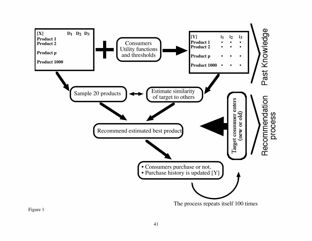
products and intelligent agents. The overall structure of the collaborative and individual simulation is

described in figures 1 and 2. Below we describe the different elements of the simulations, followed by

a description of the collaborative filtering and individual agents learning simulations.

••• Figure 1 •••

••• Figure 2 •••

The Product Catalog

We created a catalog of 1000 products [X], where each product was characterized by scores on

three positively valenced attributes, X1p, X2p, and X3p. Note that the product set is not factorial, but

rather reflects negative inter-attribute correlations (-0.3). Product choice would then be sensitive to the

8

relative weights consumers placed on the three attributes.

The Population of Consumers

At the onset of the simulation, we created a population of consumers, each defined by a vector of

preference weights for the 3 product dimensions. Because we were comparing individual to

collaborative approaches, we wanted to build a simulation in which real clusters existed. We created a

hierarchical cluster structure with three primary clusters with large mean differences in the relative

weights of the three attributes ( W s1, W s2, and W s3). Each primary cluster included three sub-

clusters with centroids that deviated from their respective primary cluster centroids. Table 2 shows the

cluster centroids for the nine segments.

Each consumer’s utility weight for dimension d, Wisd, was the sum of the consumer’s segment

mean weight ( W sd) plus a normally distributed random deviation from the segment average ,(Risd).

That is, Wisd = W sd + Risd. The Risd values were stable for each consumer i and do not vary by

product (p). Sampling randomly 20 consumers from each of the 9 segments, we created a community

population of 180 consumers.

••• Table 2 •••

Initial Product Shopping by Community Consumers

After all the consumers and products were created, all consumers “went shopping.” This

shopping process was such that each consumer (i) observed each product (p) and purchased it only if

the true overall utility of that product for that consumer exceeded that consumer’s threshold (Tip). The

threshold was set by the simulation to have a common base for all the consumers with different

random perturbations for each consumer at each product evaluation / purchase (sampled from a normal

distribution with a mean of 0 and a standard deviation that was defined by the simulation).

9

The true overall utility (U) that consumer i had for product p is given by: Uisp = S[Wisd * Xpd].

That is, the product’s score on dimension d was weighted by the consumer’s weights for dimension d.

For each of the 1000 products in the database, its utility for each consumer was computed (Uisp), and

compared to the random threshold Tip, which varied for each purchase evaluation. If Uisp > Tip, the

product p was “purchased”, and the simulation recorded a 1 for that product in the [Y] matrix column

for that consumer. If Uisp < Tip, the product was “not purchased”, and the simulation recorded a -1 in

the [Y] matrix column for that consumer.

The Target Consumer

At this point, a target consumer was generated. The preferences (weights) of this target

consumer were always sampled from segment A2 (see Table 2), where the weight of the least

important attribute remained the same for all target consumers, and the weights of the other two

attributes varied randomly around their original value in segment A2. In each simulation, this process

repeated itself for 200 different target consumers, drawing from the same distributions of random

thresholds (Tip) and the same random decision weights as the community consumers (Risd).

Recommending Products to Target Consumers

The target consumer, once created, “approached” the recommendation system and “asked” for a

product recommendation. The simulation then called one of the different intelligent agents that had

been implemented (random, K-mean, nearest-neighbor, and logistic-regression) and asked for a

product recommendation. The intelligent agent then sampled 20 products from the catalog, retrieved

all the information it had regarding these products (which differed among the various intelligent

agents), and recommended a product, which it predicts to be favored by the target consumer.

The target consumer received the recommendation, then compared Uisp to Tip and made the

10

appropriate decision. This decision was then recorded as either a buy (1) or reject (-1), and the target

consumer came back to ask for another product recommendation. This process repeated itself 100

times for each of the target consumers. Note that all agents started with diffuse priors about each

target consumer and that the mechanics of the recommendation process was identical in all 100

recommendations. Thus, changes in recommendation quality across trials can only be due to learning.

Four Algorithms for Intelligent Agents

We used four different algorithms for our intelligent agents: random, K-mean, nearest-neighbor,

and logistic-regression. Note that in all cases the recommendation engine observed only the purchase

history of 1’s and -1’s, and not any of the underlying preference information of the consumers. We

next describe each of our intelligent agents.

Random. Every time a recommendation is requested, the agent randomly samples a product and

presents it to the target consumer. The target consumer “inspected” that product, applied its own true

weights to it to compute Uisp, compared Uisp to a threshold Tip, and made the appropriate decision.

This agent did not learn; the recommendations in trials 1-100 were independent of responses made on

prior trials.

Collaborative filtering by K-mean clustering. This agent began by randomly assigning the target

consumer to one of the clusters. On each trial, the K-mean agent recommended the product that was

most frequently purchased by the other consumers in the segment to which the consumer was assigned.

The target consumer “inspected” that product, applied its own true weights to it, compared Uisp to a

threshold Tip, and made the appropriate decision. The database recorded a 1 or -1 for that product and

that consumer. The system made no record in the [Y] matrix of any information about the 19 products

that were not recommended.

As the number of recommendations increased, the agent gathered more data about the target

11

consumer, learning what segment the target consumer is most like. The consumer’s purchase history

was used to update the agent’s priors about segment membership by reclustering the target consumer

and the entire population. The agent assessed fit of the target consumer to any segment by computing

similarity for products that the target consumer had evaluated previously (with either 1 or –1 in the

consumer’s column in [Y]). The target and community were then re-clustered, using only [Y] values

for products that had been recommended to that target.

Similarity was assessed by correlation coefficients, the estimation of which requires at least two

data points. For trials 1 and 2, therefore, we used a similarity measure defined by the squared

difference between the target consumer and each of the segments. (The same approach was also used

in the nearest-neighbor approach for trials 1 and 2.)

Our simulations always extracted the 9-cluster K-mean solution. In practice, an analyst would

not know the number of clusters a priori, so our simulation was biased in favor of the clustering

approach. However, because of the random error introduced in the thresholds, Tip, and because the

utility value has been dichotomized (-1, 1), there is no guarantee that the customers (comparison or

target) will be classified into segments with others who share their true underlying preferences.

Collaborative filtering by nearest-neighbor. A nearest-neighbor approach follows a framework

just like that shown in Figure 1, except for the different algorithm for assessing which community

members to use to forecast the preferences of the target. These methods compute the correlation

between the target’s revealed preferences and those of every other consumer in the community

database (e.g., Konstan et al. 1997; Good et al. 1999). This approach is called “nearest-neighbor”

because the most similar persons in the community are used more heavily to predict reactions of the

target consumer (Breese et al. 1998; Gershoff and West 1998).

In our simulations, a similarity matrix was created between the target consumer and the

12

population of consumers, and the weight given to each of the consumers in the population was

proportional to the similarity of their purchase pattern in [Y] from the pattern of the target consumer.

The decision process of the target consumers, the repetitions, and the information recorded in the

database were otherwise exactly the same as the K-mean clustering.

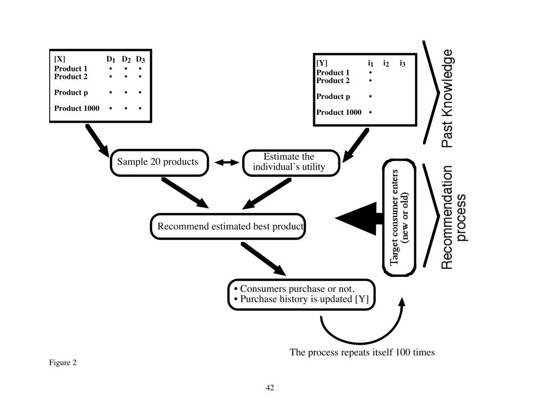
Individual-based logistic-regression intelligent agents. The simulation for the individual-based

intelligent agent mimics the simulation for the community-based intelligent agent with two main

differences (see Figure 2). In the individual agent, there is no initial set of “population” consumers.

We only make use of the column from the [Y] matrix for the “target” consumer. Second, the

recommendation technique is different. The agent does not rely on the target consumer’s assumed

similarity to others to forecast liking for a new product. Instead, the agent performs a logistic-

regression of the purchase / no purchase (1, -1) values in [Y] on the associated X values for those

products, estimating the target’s utility weights (Wisd) for the sampled products, and recommend the

product with the highest expected utility (Uisp).

The logistic regression model requires the estimation of 4 parameters. On trials 1-3, the

simulation used a reinforcement learning bootstrap, beginning with an equal weight model and then

reinforcing or inhibiting the weights of the consumer to account for the reaction to each new

recommendation.

Dependent Variable

There are two types of success measurements we can get from the simulation. First, we can

measure the probability of purchasing – i.e., the probability that the utility of the recommended product

exceeds Tip. Second, we can compare the performance of the agent to an omniscient who always

recommended the product with the highest utility for the target consumer (Uisp). Note that this second

13

measure can only be available in a simulation. In our simulation, these two measures produced

identical conclusions about the effects of the independent variables described below. Thus, for brevity,

we present only the “probability of purchasing” results.

RESULTS

Performance When Tastes and Product Alternatives are Stable

Our major focus is on the differential learning characteristics of individual vs. community based

collaborative agents. We begin by comparing K-mean, nearest-neighbor, logistic-regression, and

random agents under conditions where neither the consumer nor the environment change over time.

We report “success” (probability of buying the recommended option) over time; we do not report

inferential statistics because of our arbitrarily large sample sizes.

Baseline comparison of four recommendation agents. Figure 3 compares success over trials 1 to

100 for our three types of agents vs. a null model where recommendations were random. Success rate

is the percent of recommended products that are purchased because they exceeded the target

consumer’s utility threshold. The simulation was set such that 20% of the products in the catalog

exceeded the expected value of the errorful utility thresholds. Consequently, the bottom curve in

Figure 3 shows that an agent who recommends products randomly has a 20% success rate that does not

improve over time. The top curve (triangles) shows the performance of an individual logistic-

regression agent. The two curves below it show two kinds of collaborative filters: the nearest-neighbor

agent (squares) and the K-mean agent (circles).

As can be seen in Figure 3, the nearest-neighbor agent outperforms the K-mean agent by roughly

7%, and this advantage exists from trial 1 to trial 100. The individual agent performs at a lower level

than either collaborative agents until roughly trial 20, but its asymptotic success rate of 80% is

14

substantially higher than either collaborative method. Thus, it appears that collaborative filter

algorithms achieve modest success more quickly than an individual agent, but are substantially

outstripped by individual agents in the long run.

Note that in our simulation, this crossover point occurred after 20 trials, but this is a function of a

number of simulation details. It should increase if the [X] matrix is missing key attributes or

interactions, if the utility function is of high dimensionality, or if the number of segments is smaller

than the 9 used here. It should be obvious to the reader, for example, that if the [X] matrix excluded

enough key predictors, the individual agent might never exceed the intercept of the collaborative

filters.

For each curve, we estimated the parameters of a learning function with an intercept, an

asymptote, and a rate parameter capturing the speed with which learning moved from intercept to

asymptote. A convenient functional form is the modified exponential (Lilien, Kotler, and Moorthy

1992, p. 656): Proportion Success (t) = a + c [1 - e -b * t]. In this function, there is one independent

variable, t = trial number, and three parameters to be estimated. The intercept (a) is the predicted

success at trial t = 0, before any feedback has occurred; c is the change in performance from trial 0 to

the asymptote (which is a + c). The rate of learning is captured in parameter b; [1 - e –b ] can be

interpreted as the proportion of the potential learning remaining at trial t that occurs after one

incremental trial. Values of [1 - e –b] close to 1 reflect very fast learning, almost like a step function

rising to asymptote in the first few trials; values close to 0 reflect slow learning, nearly linear

throughout the trials. If the asymptotic success rate is (a + c), the remaining potential learning at time

t is [a + c – proportion success (t)]; [1 - e –b] is the expected fraction of remaining potential achieved

on each trial, t. We recoded trial numbers 1 to 100 to 0 to 99 to make intercepts reflect first trials.

In Table 3, we show the parameters of this function and the associated standard errors for our

15

three intelligent agents and the random recommendation baseline. The parameter values should be

treated as descriptive and not inferential statistics, since one could arbitrarily add consumers to the

simulation to reduce the noise around the aggregate mean data points and reduce standard errors. The

R2 values give a sense of how well this learning function captures the change in aggregate success over

trials for each agent. Fit is better for the logistic-regression agent because there is more total variance

in success to be explained by trials. For random recommendations, there is minimal variance over

trials in success rate and none of it is systematic, as shown by the R2 of zero.

Intercepts (a). As shown in Figure 3, the intercepts for the two collaborative filters exceeded .2,

the success rate for a random recommendation. This is because our product catalog is not maximally

“efficient” (attribute correlations = -0.3, and the maximum average negative correlation among three

attributes is -.5; Krieger and Green 1996). Thus, the product catalog included some products with

exceptionally good or bad attribute values for all segments, which made it likely that the best product

out of 20 will have a high mean utility for other segments. Thus, collaborative approaches can have an

initial bootstrap based on the population evaluation even when there is no information about the target

consumer (cf. Ansari et al. 2000). The individual-based logistic-regression agent lacks this initial

advantage. Its success rate is .2 until it can collect enough data points to estimate the coefficients of

the model.

Total learning (c). As information accumulated about the target consumer, the individual

logistic-regression improved quickly overcoming its initial disadvantage (c = .75), and outperforming

the other agents at its asymptote (a + c = .80). Among the two collaborative filtering approaches the

nearest-neighbor does better in terms of higher total learning than the K-mean agent (.37 vs. .22) and

asymptotic level of success (.58 vs. .50, respectively).

Learning rate (b). Collaborative filter agents reach their success asymptote much faster than the

16

individual agent. Recall that [1 - e -b ] is the proportion of the remaining available learning that

occurs per trial. A higher value of b implies that learning is “front loaded”; a bigger proportion of the

learning that will ever occur happens on each early trial, leaving less learning “available” for later

trials. The [1 - e -b ] values for nearest-neighbor, K-mean, and the individual logistic-regression are

.10, .15, and .06, respectively, implying that collaborative filters are more “front-loaded.”

••• Figure 3 and Table 3 •••

K-mean Agent and Sticky Initial Classifications

We attribute the lower total learning, c, and the higher learning rate, b, evident in the K-mean

agent to stickiness in the classification of a respondent into a cluster. We propose that cluster based

collaborative filters learn less than one might expect because they remain stuck on the image they first

“see” when they classify a target consumer into a cluster, and because feedback from (mostly sub-

threshold) recommendations is not sufficiently diagnostic for reclustering. Recall that on the first trial,

consumers were randomly assigned to a cluster and were recommended the product most suitable to

that cluster. Because there were 9 clusters, the odds of being correctly classified were 1/9. Therefore,

the percentage of customers that should have remained classified in the same cluster throughout trials

1to 100 should have been 11.1%. Instead, we found that 29.5% of consumers did not change clusters

from trial 1 to trial 100. Classifications were even stickier when a very small amount of data had been

collected; from trial 2 to trial 100, 37.5% did not change their cluster; from trial 5 to trial 100, 48% did

not change their cluster. This pattern was consistent with the high values of the learning rate

parameter, b and the front loaded learning.

Why did stickiness occur? Collaborative filters produce a systematic a bias toward

nondiagnostic evidence when recommendations are based upon what is “best” under the currently

maintained hypothesis. The statistical properties are very similar to the learning from feedback

17

mechanisms postulated by March’s (1996, p. 315) research on why people incorrectly learn to be risk

averse from feedback from choice of risky vs. riskless options.

“Much of the power of learning stems from these sequential sampling properties. By shifting

sampling from apparently inferior alternatives to apparently superior ones, the process improves

performance. However, these same properties of sequential sampling complicate learning from

experience. An experiential learning process reduces the rate of sampling apparently inferior

alternatives and thus reduces the chance to experience their value correctly, particularly for those with

high variance in returns. Correction in estimates of expected return from each alternative is a natural

consequence of the unfolding of experience, but it is inhibited by any learning process that quickly

focuses choice and thus reduces the sampling rate of one alternative.”

The logistic-regression agent also tends to recommend only products that are consistent with the

utility weights estimated for the target. However, the key difference is that this does not prevent the

observed response from correcting the utility weights. Success causes an increased weight on

attributes that happen to be strong for the accepted product and a decreased weight on weaker

attributes, relative to other recommended products in that customer’s database. We believe that this

explains the logistic-regression’s higher total learning, c, and less front-loaded learning rate, [1 - e -b ],

in comparison with collaborative filters.

Effects of an Consumer’s Distance from Cluster Average Utility Weights

Since the K-mean agent is the most common type of agent in most commercial applications, it is

interesting to note that its performance is relatively poor in our simulations. Why? The agent makes

recommendations based on the average behavior of the consumers in the segment to which the target

consumer is assigned. The upper limit its predictive accuracy is related to the correlation between the

consumers’ preferences and the preferences of the average consumer within their segment (assuming

18

classification is accurate). Consumers whose preferences are farther from their cluster center will be

predicted less well than those close to the center.

For the nearest-neighbor collaborative filter, predictive accuracy will be unaffected by the

similarity between the consumer’s utility weights and those of the average consumer in the same

cluster. Nearest-neighbor algorithms make use of similar consumers independent of their cluster

typicality.

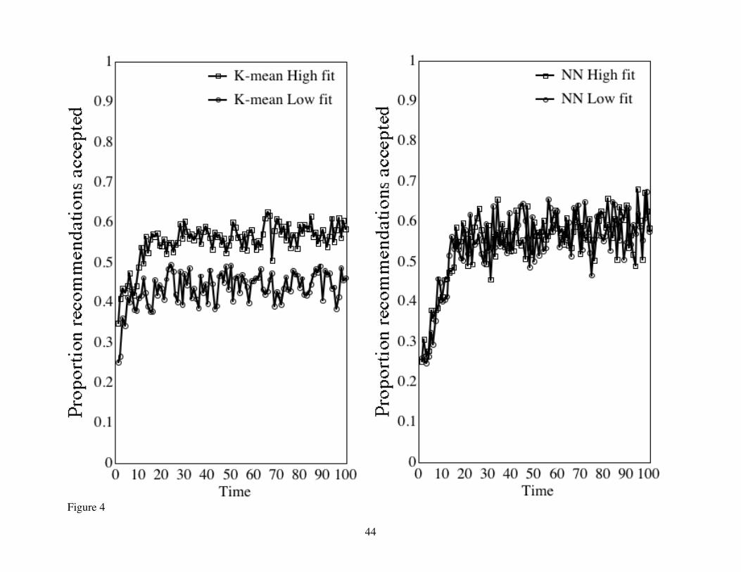
Figure 4 illustrates both of these points. We stratified the results from Figure 3 for the K-mean

and nearest-neighbor agents according to the degree to which the consumer’s utility weights departed

from the average weights of the cluster to which the target was assigned. In the utility function Uisp =

S(Wisd * Xpd) = S[( W sd + Risd )* Xpd], “high fit consumers” had Risd values in the two central

quartiles. “Low fit consumers” had Risd values in the two extreme quartiles.

Table 4 shows that, for the K-mean agent, the asymptotic level of learning is significantly lower

for consumers that are atypical of their cluster. The higher asymptotic levels of accuracy for high fit

vs. low fit consumers, (.57 vs. .44, respectively) is primarily due to the difference in their intercepts

(.36 vs. .26, respectively) and to learning that approaches its asymptote faster in low-fit than in high-fit

conditions. Note that (1 - e –b ) = .20 and .11 for low and high-fit, respectively.

In contrast, the performance of the nearest-neighbor agent is unaffected by the consumer’s fit,

with a asymptotic success rate of .58 for both high and low fit consumers. Note that this asymptote is

nearly identical to that in K-mean for high fit consumers. In other words, for target consumers who are

typical of their clusters, these two algorithms will yield closely correlated predictions, but in cases

where there are also atypical consumers, the nearest-neighbor algorithm will perform best.

••• Figure 4 and Table 4 •••

Another simulation made a related point. We manipulated the within-segment variance in

19

weights for the three attributes (Risd). When this variance = 0, all consumers in a segment have

identical weights. Here, K-mean asymptotic performance (.534) approached that of nearest-neighbor

(.579). Nearest neighbor asymptotes were unaffected by within-segment variance is weights.

Error in Reservation Utility Thresholds for Target Consumers and Community

Consider the effect of adding noise to the dependent variable of response to recommendations, as

occurs, for example, when agents rely on “implicit” rather than “explicit” response to

recommendations (Nichols 1997). In our simulations, we assume that consumers assess without error

their utility for product p, but that there is error in the translation from utility to purchase. A

recommended product p is purchased if it’s utility exceeds an errorful reservation threshold– i.e., if

Uisp > Tip. The threshold has a mean value but varies randomly among consumers and products, so

that the same recommended product could be accepted by a consumer in one trial but rejected in

another. We refer to this noise in thresholds as “purchase error”, and compare the performance of our

three agents as the variance around the mean threshold to increase from 5 (in the base case shown in

Figure 3) to 15. In our two collaborative filtering simulations (K-means clustering and nearest-

neighbor), the same purchase error variance in Tip is assumed for the community and for the target

consumer. Results are shown in Figure 5 and Table 5.

For all three agents, asymptotic proportions of recommendations that are successful (a + c) is 0.1

to 0.2 lower when there is more noise in the purchase thresholds. However, the focus of the deficit

varies from agent to agent.

All three agents gain less from intercept to asymptote when there is more error in purchase

threshold and therefore in purchasing responses (see parameter c in Table 5). For logistic-regression,

the expected value of the coefficients for the 3 dimensions is unaffected by error in the dependent

variable, yet the effect of purchase error is asymmetric for positive and negative changes to the

20

threshold. When purchase error decreases the threshold, the probability of purchase remains high and

relatively unaffected. But when purchase error increases the threshold, it becomes more likely that

Uisp < Tip – hindering success.

For K-mean and nearest-neighbor, the asymptotic level of success is closer to .5, such that there

is no asymmetric effect of positive and negative threshold errors, and increasing purchase error

decreases success for a different reason. For K-mean, purchase error increases the chance that the

consumer will be classified into the wrong segment. Because of the endogenous generation of

nondiagnostic feedback we noted earlier, such misclassifications are long-lived. Similar mechanisms

cause the c values for nearest-neighbor to be depressed by purchase error, which causes the target’s

preferences to be predicted by consumers whose utility weights are less similar to their own.

In K-mean, increasing the purchase error also decreases the learning rate parameter, b, from .16

to .04. The latter implies that with noisier purchase thresholds, learning approaches asymptote more

slowly. This result is due to the fact that the clusters themselves have a large error component and are

thus less diagnostic and less stable.

••• Figure 5 and Table 5 •••

Agent Learning When Tastes Change

In all of the simulations described thus far, the target consumer had a single, stable utility

function guiding purchase or nonpurchase of recommended products across all 100 trials. However, a

major problem for intelligent agents is that the database purchase history may include purchases

governed by different utility functions. The consumer may experience a permanent change in

circumstances, e.g., from graduation, a move, or change in stage of the family life cycle (Wilkes 1995),

or may have different attribute weights depending on the usage situation (Dickson 1982; Miller and

Ginter 1979). When a single agent attempts to model the mixed purchase stream, aggregation errors

21

can result. We next compare individual and collaborative approaches in their sensitivity to such

changes in taste.

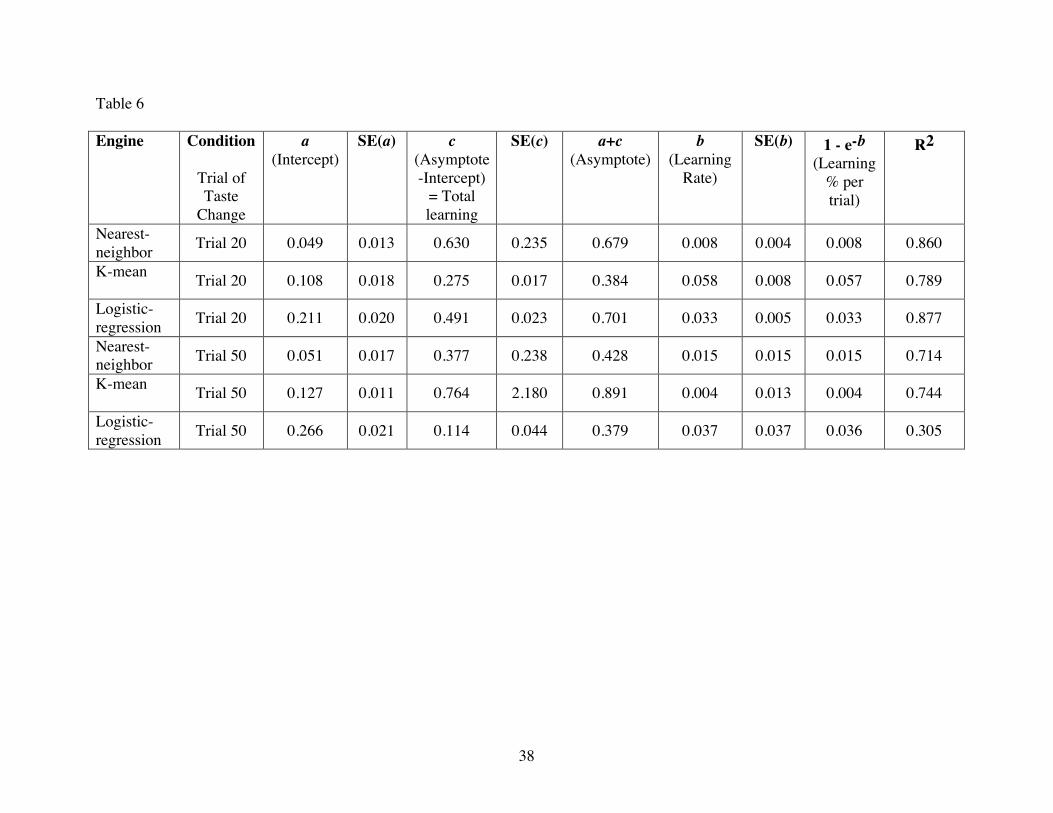
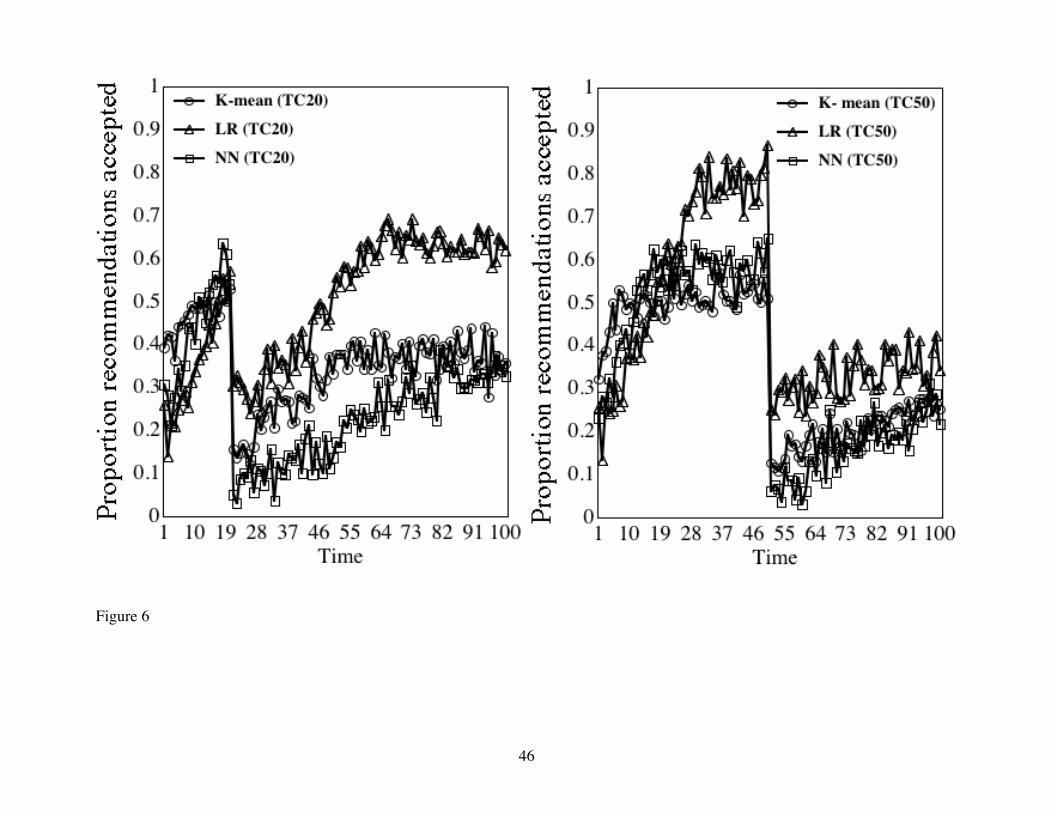
We tested a simple form of aggregation error: whether the consumer‘s tastes changed

permanently after a given number of learning trials. After either 20 learning trials (Figure 6a and

Table 6, top) or after 50 trials (Figure 6b and Table 6, bottom), we changed each target consumer’s

utility function from centering around sub-segment A2 to centering around sub-segment C2 (see Table

3). Figure 6 shows that, by 20 trials, all three agents are predicting at about a 50% success rate, with a

slight advantage to the nearest-neighbor agent. After the taste change, nearest-neighbor’s predictive

accuracy is the worst of the three, and logistic-regression is best. Eventually, nearest-neighbor again

catches up to, and surpasses K-mean agent.

Figure 6b shows that, after 50 trials, all three agents have learned substantially. After the taste

change, nearest-neighbor’s predictive accuracy is the worst of the three, but logistic-regression has

suffered the largest overall decrease in accuracy. It is also interesting to note the differences in

learning rates between the first 50 trials and the last 50 trials. In the last 50 trials, all three agents base

their recommendations on all the data (before and after the taste change) and therefore, learning is

slower.

Why is the individual agent less adversely affected in the long run? Logistic-regression differs

from the two collaborative filters in its propensity to recommend options that lead to feedback that

corrects errors in initial hypotheses. With 20 trials worth of feedback under the consumer’s original

utility function, all agents recommend products predicted to be the best of 20 sampled on trial t under

the old hypothesis. For collaborative filters, it becomes extremely unlikely that a recommendation will

be made that is very diagnostic – i.e., one where acceptance or rejection produces a likelihood ratio

strongly favoring the new and more accurate hypothesis. In logistic-regression though, both success

22

and failure produce continuous correction after the consumer’s utility weights have shifted. Success

increases the weight of attributes on which the purchased product is high, and decreases the weight of

attributes on which the purchased product is low. The opposite is true for failure.

••• Figure 6, Table 6 •••

GENERAL DISCUSSION

Limitations

The conclusions from this research should be understood to be a function of a number of

simulation design decisions that affect either main effect differences among agent types, or their

interactions with trials (feedback) and the independent variables we manipulated.

- Performance of the different agents in our simulations depends in part on the correlations among

the attributes. If attributes are less negatively correlated and there are more dominated and

dominating alternatives, collaborative filters will easily identify and recommend products liked by

everyone, leading to a higher intercept. More negative correlations have the opposite effect.

- Performance of the different agents in our simulations depends in part on the degree of overlap

between consumers and clusters. Our clusters had modest overlap; consumers from two different

clusters could have quite similar weights. Less overlap should make easier the task of K-mean but

leave learning by nearest-neighbor and logistic-regression agents unaffected. We showed above

that such effects are slight. With zero within-cluster variance in weights, K-mean came closer to

the asymptotic performance of nearest-neighbor, but remained far below the performance of the

logistic-regression.

- The utility function for our products was simple, with three attributes with no interactions. A

logistic-regression agent with more parameters would have required more trials to match and

23

surpass the accuracy of our collaborative filters.

- Our [X] matrix had complete information for all attributes included in the utility function.

Collaborative filters are often used in circumstances where key attributes are absent, subjective, or

proprietary. If the variables in our [X] matrix collectively explained little variance in utility, the

gain from learning (c) would have been diminished for the logistic-regression but not for

collaborative filters.

- Our simulation had 9 clusters. Fewer clusters would have increased total learning for K-mean, with

no effects on the other two kinds of agents. This is because, with fewer clusters, negative feedback

from an initial wrong classification would be more diagnostic because it’s updating value would

not be spread across many alternative hypotheses compatible with rejection. Fewer clusters would

reduce the stickiness of original classifications.

- Our community size of 180 members corresponds to an early stage of growth in a collaborative

filter. Shandanand and Maes (1995), for example, report that their “Ringo” agent attracted 1000

users in its first month. Having more community members would help learning by collaborative

filters.

- Our community has far more data per user than is typical, with complete responses to all 1000

products for each member. This favors the collaborative filters and reduces cold start problems.

Conclusions

The major conclusion from this work is that individual agents and collaborative filters have

different learning properties. It is not our goal to declare one type of agent as superior; after all,

several authors have been working on combining individual and collaborative approaches into a single

agent (e.g. Chung and Rao 2001; Good et al. 1999; Popescul et al 2001; Schein et al. 2002). Our aim is

24

to better understand what factors affect the rates at which different pure types of agents learn from

feedback to recommendations generated by the agent.

Comparing collaborative filters, we showed that K-mean agents learn about as well as nearest-

neighbor for consumers who are close to the centroids of their clusters, but less well for consumers

farther from cluster centroids. Compared to collaborative filters, individual agents: 1) learn slower

initially, but are better off in the long run if the environment is stable; 2) recover faster after a

permanent changes in the consumer’s utility function; 3) are less adversely affected by random error in

the purchase thresholds that makes purchase a noisy indicator of underlying utility functions.

These conclusions do not necessarily imply that collaborative agents are inferior. We noted

above many circumstances under which collaborative agents might have higher asymptotic

performance, and we showed that collaborative systems perform better initially when the agent has

little or no information about the consumer.

Given the relative performance of the collaborative and individual agents, it might be suggested

that the best approach for smart agents is to base their recommendations on a mixture of these two

approaches is best: when there is little or no knowledge, rely on the collaborative component, but as

information about a consumer accumulates, the recommendations of individual agents should pervail.

This type of recommendation has one central flaw: As was shown earlier, recommendations of agents

also define the agent’s own learning environment. Thus, it is not clear that a switch from collaborative

filers to individual agents can provide the same learning potential as when an individual agent was

used throughout. In sum, the question of when and how to use these two types of agents is still open.

Unresolved Issues and Future Research

In considering what approach to use, another key factor is what are consumers’ requirements in

25

terms of recommendation quality. At what level of recommendation quality will consumers persist

using an intelligent agent and at what level will they abandon recommendation systems? The

designers of such systems would prefer (hope) that consumers would judge agents positively if they

provide better than random recommendations. We suspect that this is not the case, and in fact that

consumers are likely to judge performance negatively as it deviates from their high expectations

(100%?). Understanding the recommendation level that will satisfy consumers is important because

providing tentative initial recommendations might be self-defeating.

The simplest method for avoiding low-quality recommendations is to withhold recommendations

until the agent has sufficient information to make high quality recommendations. In order to accelerate

learning, the agent can explicitly ask consumers to provide feedback (ratings, choices) about products

they like and dislike. By using this input as a starting point for the estimation procedures before

making any recommendations, an agent can start the learning curve at a higher level of initial

recommendation quality. How many questions and how much time will consumers be willing to

spend, and under what conditions (one vs. multiple sessions etc.)? Future research is also needed to

understand circumstances under which consumers will be willing to train agents rather than abandon

them for poor initial recommendation quality. In addition to withholding recommendations and asking

for explicit input, agents can frame the recommendations as tentative, indicating to the consumer that

more learning needs to take place before high quality recommendations can be made. We might ask

here is whether consumers will be more forgiving for recommendations that are framed as tentative,

and whether they will be willing to keep on using such systems until they mature.

Another key research question emerges from the stickiness of essentially random classifications

in K-mean agent (Statgraphics). The question here is how to design agents that can learn more

efficiently without getting stuck in local sub-optima. It is clear that the goal of short-term

26

maximization of recommendations is in conflict with the long-term goal of learning the consumer’s

preferences. One can envision a “multiple-armed bandit” (DeGroot 1970) approach to

recommendations, balancing expected success over a stream of future trials and not just the current

trials. For one such approach, see Oliveira (2002). In addition, a similar methodology might be used to

recommend multiple rather than single products, where options in the recommended set are chosen to

maximize learning. Understanding how to balance short-term recommendation acceptance with long-

term learning, and how to use multiple simultaneous recommendations for maximizing learning

deserves future investigation.

Finally, research is needed on learning to detect taste changes. As can be seen in Figure 6, the

learning speed after the change occurred is much lower compared to the initial learning speed. As

stated earlier, this is due to faulty estimates generated by incorporating the old (irrelevant) purchase

history into predictions. Learning could be improved if the agent simply forgot the old data by one of

three possible approaches. First, an agent can always give higher weight to the most recent feedback.

Alternatively, an agent can measure its own success over the past N trials against expected success,

based on the learning function to date. Once success is found to be significantly below expectation (as

in Figure 6), the agent can take this as an indication that the preference structure has changed and

actively forget the old information. Finally, an agent can use latent learning principles whereby there

is no forgetting per se, but rather a classification of old and nondiagnostic information into a category

that is familiar, but also known to have no influence on behavior. The advantage of such an approach

is that if circumstances change, the old information could become easily available again. Optimal

forgetting functions could be a rich avenue for future research.

27

REFERENCES

Alba, Joseph, John Lynch, Barton Weitz, Chris Janiszewski, Richard Lutz, Alan Sawyer, and Stacy

Wood (1997), “Interactive Home Shopping: Consumer, Retailer, and Manufacturer Incentives to

Participate in Electronic Marketplaces,” Journal of Marketing, 61 (July), 38-53.

Ansari, Asim, Skander Essegaier, and Rajeev Kohli (2000), “Internet Recommender Systems,” Journal

of Marketing Research, (August) 363-375.

Avery, Christopher, Paul Resnick, and Richard Zeckhauser (1999), “The Market for Evaluations,”

American Economic Review, 89 (June), 564-584.

Balabanovic, Marko and Yoav Shoham, (1997), “Fab: Content-Based, Collaborative

Recommendation,” Communications of the ACM, 40 (March), 66 – 72.

Breese, John S., David Heckerman, and Carl Kadie (1998), “Empirical Analysis of Predictive

Algorithms for Collaborative Filtering,” Proceedings of the 14th Conference on Uncertainty in

Artificial Intelligence, Madison, WI 1998; San Francisco, Morgan Kaufmann Publisher, 43-52.

Condliff, Michell Keim, David D. Lewis, David Madigan, and Christian Posse (1999), “Bayesian

Mixed-Effects Models for Recommender Systems,” ACM SIGIR ’99 Workshop on Recommender

Systems: Algorithms and Evaluation, University of California, Berkeley, August 19, 1999.

DeGroot, Morris H.. (1970) Optimal Statistical Decisions. New York-London-Sydney: McGraw Hill.

Dickson, Peter R. (1982) “Person-Situation: Segmentation’s Missing Link,” Journal of Marketing, 46

(4), 56-64.

Diehl, Kristin R., Laura J. Kornish, and John G. Lynch, Jr. (in press), “Smart Agents: When Lower

Search Costs for Quality Information Increase Price Sensitivity,” Journal of Consumer Research.

Gershoff, Andrew, and Patricia M. West (1998), “Using a Community of Knowledge to Build

Intelligent Agents,” Marketing Letters, 9 (January), 835-847.

28

Goldberg, David, Brian Nichols, Brian M. Old, and Douglas Terry (1992), “Using Collaborative

Filtering to Weave an Information Tapestry,” Communications of the ACM, 35 (December), 61-70.

Good, Nathaniel, J. Ben Schafer, Joseph A. Konstan, Al Borchers, Badrul Sarwar, Jon Herlocker, and

John Reidl (1999), “Combining Collaborative Filtering with Personal Agents for Better

Recommendations,” Proceedings of the 1999 Conference of the American Association of Artificial

Intelligence (AAAI-99), 439-446.

Häubl, Gerald, and Valerie Trifts (2000), “Consumer Decision Making in Online Shopping

Environments: The Effects of Interactive Decision Aids,” Marketing Science, 19 (1).

Herlocker, Jonathan L, Joseph A. Konstan, Al Borchers, and John Riedl (1999), “An Algorithmic

Framework for Performing Collaborative Filtering,” Proceedings of the 1999 Conference on

Research and Development in Information Retrieval. Association for Computing Machinery.

Hill, Will, Larry Stead, Mark Rosenstein, and George Furnas (1995), “Recommending and Evaluating

Choices in A Virtual Community of Use,” Human Factors in Computing Systems, CHI ‘95

Conference Proceedings, ACM, 194-201.

Iacobucci, Dawn, Phipps Arabie, and Anand Bodapati (2000), “Recommendation Agents on the

Internet,” Journal of Interactive Marketing, 14 (3), 2-11.

Jacoby, Jacob, Donald E. Speller, and Carol Kohn Berning (1974), Brand Choice Behavior as a

Function of Information Load: Replication and Extension, Journal of Consumer Research, 1

(June), 33-42

Konstan, Joseph A., Bradley N. Miller, David Maltz, Jonathan Herlocker, Lee R. Gordon, and John

Riedl (1997), “GroupLens: Applying Collaborative Filtering to USENET News,” Communications

of the ACM, 40 (March), 77-87.

Krieger, Abba M. and Paul E. Green (1996), “Linear Composites in Multiattribute Judgment and

29

Choice: Extensions of Wilks' Results to Zero and Negatively Correlated Attributes,” British

Journal of Mathematical and Statistical Psychology, 49 (May, Part 1), 107-126.

Lilien, Gary L., Philip Kotler, and K. Sridhar Moorthy (1992), Marketing Models. Englewood Cliffs,

NJ: Prentice Hall.

March, James G. (1996), “Learning to Be Risk Averse,” Psychological Review, 103 (2), 309-319.

Miller, Kenneth E. and James L. Ginter, (1979), “An Investigation of Situational Variation in Brand

Choice Behavior and Attitude,” Journal of Marketing Research, 16 (1), 111-123

Nichols, David M. (1997), “Implicit Rating and Filtering,” in European Research Consortium for

Informatics and Mathematics, Fifth DELOS Workshop Filtering and Collaborative Filtering,

ERICM Workshop Proceedings, No. 98-W001.

Oliveira, Paulo R. (2002) “Service Delivery and Learning in Automated Interfaces.” Unpublished

Ph.D. Dissertation, Massachusetts Institute of Technology, Cambridge, MA.

Popescul, Alexandrin, Lyle H. Ungar, David M. Pennock, and Steve Lawrence (2001), “Probabilistic

Models for Unified Collaborative and Content-Based Recommendation in Sparse-Data

Environments,” In Proceedings of the 17th Conference on Uncertainty in Artificial Intelligence

(UAI 2001), Seattle, WA, August 2001.

Rich, Elaine (1979), “User Modeling via Stereotypes,” Cognitive Science, 3, 335-366.

Schafer, J. Ben, Joseph Konstan, and John Riedl (1999), “Recommender Systems in E-Commerce.”

Proceedings of the ACM Conference on Electronic Commerce, November 3-5, 1999.

Schafer, Joseph L and John W. Graham (2002), “Missing Data: Our View of the State of the Art,”

Psychological Methods, 7 (2), 147-177.

Schein, Andrew I, Alexandrin Popescul, Lyle H. Ungar, and David M. Pennock (2002), “Methods and

Metrics for Cold Start Recommendations,” SIGIR ’02, August 11-15, Tampere, Finland.

30

Shardanand, Uprendra and Pattie Maes (1995), “Social Information Filtering: Algorithms for

Automating ‘Word of Mouth’,” Proceedings of the Conference on Human Factors in Computing

Systems (CHI ‘95), ACM Press, 210-217.

West, Patricia M., Dan Ariely, Steve Bellman, Eric Bradlow, Joel Huber, Eric Johnson, et al. (1999),

“Agents to the Rescue?” Marketing Letters, 10 (3), 285-300.

Wilkes, Robert E (1995), “Household Life-Cycle Stages, Transitions, and Product Expenditures,”

Journal of Consumer Research, 22 (June), 27-42.

31

AUTHOR NOTE

Dan Ariely: Massachusetts Institute of Technology, 38 Memorial Drive E56-329, Cambridge, MA

02142; Tel (617) 258-9102 Fax (617) 258-7597; ariely@mit.edu, web.mit.edu/ariely/www.

John Lynch: Fuqua School of Business, Duke University, Box 90120, Durham, NC 27708-0120;

Tel (919) 660-7766 Fax (919) 681-6245; john.lynch@duke.edu, www.duke.edu/~jglynch.

Manuel Aparicio: Saffron Technology, 1600 Perimeter Park Dr. Suite 150. Morrisville, NC 27560;

Tel (919) 468-8201 Fax (919) 468-8202; maparicio@saffrontech.com, www.saffrontech.com.

The authors would like to thank Carl Mela, Shane Frederick, Robert Zeithammer, the Editor, and the

reviewers for their comments, as well as the Center for eBusiness at MIT’s Sloan School of

Management and the e-markets Special Interest Group at the MIT Media Lab for their support.

32

Table Captions

Table 1: Product attribute matrix [X] and ratings matrix [Y] used for intelligent recommendation

agents. In [X], rows are products and columns are dimensions of products. In [Y], rows are products

and columns are consumers making product ratings.

Table 2: Starting values for the preferences of the population. The table shows the three main

segments and their three sub-segments and the weights they place on attribute dimensions X1, X2, and

X3.

Table 3: Parameter estimation for the data in Figure 3. Proportion Success = a + c [1 - e -b * t]. Base

case in which target’s tastes are stable over t = 1 to 100 trials.

Table 4: Parameter estimation for the data in Figure 4. Proportion Success = a + c [1 - e -b * t].

Comparison of fit of K-mean and nearest-neighbor for consumers with high vs. low fit to segment’s

centroid. High fit consumers have utility weights in the middle two quartiles of the segment’s

distribution, and low fit consumers are in highest and lowest quartiles.

Table 5: Parameter estimation for the data in Figure 5. Proportion Success = a + c [1 - e -b * t].

Effects of increased “purchase error” in thresholds Tip on recommendation success by logistic-

regression, K-mean, and nearest-neighbor agents.

Table 6: Parameter estimation for the data in Figure 6. Proportion Success = a + c [1 - e -b * t].

Effects of permanent change in target’s utility weights on trial 20 (Figure 6b) or trial 50 (Figure 6b) on

recommendation success by logistic-regression, K-mean, and nearest-neighbor agents. Model fits re-

code time period of trial to define t = 0 as first period after “taste change.”

33

Table 1

X1 X2 … Xd … XD Ind1 Ind2 … Indi … IndN

Product 1 Product 1Product 2 Product 2

… [X] … [Y]Product p Product p

… …Product P Product P

34

Table 2

Segment A Segment B Segment C

AttributeDimension

X1 X2 X3 X1 X2 X3 X1 X2 X3

Sub-Segment 1 50 45 5 5 50 45 45 5 50

Sub-Segment 2 50 35 15 15 50 35 35 15 50

Sub-Segment 3 50 25 25 25 50 25 25 25 50

35

Table 3

Engine Condition a(Intercept)

SE(a) c(Asymptote-Intercept)

= Totallearning

SE(c) a+c(Asymptote)

b(Learning

Rate)

SE(b) 1 - e-b(Learning

% pertrial)

R2

Nearest-neighbor

A (Base) 0.212 0.020 0.367 0.019 0.579 0.108 0.010 0.103 0.846

K-mean A (Base) 0.282 0.017 0.222 0.017 0.504 0.157 0.020 0.146 0.730

Logistic-regression

A (Base) 0.059 0.022 0.745 0.021 0.804 0.057 0.003 0.056 0.942

Random A (Base) 0.203 0.002 0.000 0.000 0.203 0.000 0.000 0.000 0.000

36

Table 4

Engine Condition a(Intercept) SE(a)

c(Asymptote-Intercept)

= Totallearning

SE(c) a+c(Asymptote)

b(Learning

Rate)SE(b)

1 - e-b(Learning

% pertrial)

R2

K-mean High fit 0.364 0.016 0.208 0.016 0.572 0.116 0.015 0.109 0.731

K-mean Low fit 0.261 0.024 0.183 0.024 0.443 0.221 0.049 0.198 0.465

Nearest-neighbor High fit 0.226 0.026 0.354 0.026 0.579 0.106 0.013 0.101 0.740

Nearest-neighbor Low fit 0.199 0.027 0.381 0.027 0.579 0.110 0.013 0.104 0.758

37

Table 5

Engine Condition a(Intercept)

SE(a) c(Asymptote-Intercept)

= Totallearning

SE(c) a+c(Asymptote)

b(Learning

Rate)

SE(b) 1 - e-b(Learning

% pertrial)

R2

Logistic-regression

A (Base)0.059 0.022 0.745 0.021 0.804 0.057 0.003 0.056 0.942

Logistic-regression

HighPurchaseError

0.052 0.022 0.655 0.021 0.707 0.050 0.004 0.048 0.921

K-mean A (Base)0.282 0.017 0.222 0.017 0.504 0.157 0.020 0.146 0.730

K-mean HighPurchaseError

0.297 0.014 0.106 0.013 0.403 0.035 0.012 0.034 0.395

Nearest-neighbor

A (Base)0.212 0.020 0.367 0.019 0.579 0.108 0.010 0.103 0.846

Nearest-neighbor

HighPurchaseError

0.241 0.015 0.148 0.015 0.389 0.102 0.018 0.097 0.588

38

Table 6

Engine Condition

Trial ofTaste

Change

a(Intercept)

SE(a) c(Asymptote-Intercept)

= Totallearning

SE(c) a+c(Asymptote)

b(Learning

Rate)

SE(b) 1 - e-b(Learning

% pertrial)

R2

Nearest-neighbor Trial 20 0.049 0.013 0.630 0.235 0.679 0.008 0.004 0.008 0.860

K-mean Trial 20 0.108 0.018 0.275 0.017 0.384 0.058 0.008 0.057 0.789

Logistic-regression Trial 20 0.211 0.020 0.491 0.023 0.701 0.033 0.005 0.033 0.877

Nearest-neighbor Trial 50 0.051 0.017 0.377 0.238 0.428 0.015 0.015 0.015 0.714

K-mean Trial 50 0.127 0.011 0.764 2.180 0.891 0.004 0.013 0.004 0.744

Logistic-regression Trial 50 0.266 0.021 0.114 0.044 0.379 0.037 0.037 0.036 0.305

39

Figure Captions

Figure 1: An illustration of the community-based intelligent agent. The brackets on the

right represent the two different aspects of the simulation: 1) creating the products and the

database; 2) making the recommendations, and obtaining the measurements. The dots in the

databases represent data being used by the community-based intelligent agents (names of the

products and their evaluations by the community).

Figure 2: An illustration of the individual-based intelligent agent. The brackets on the

right represent the two different aspects of the simulation: 1) creating the products and the

database; 2) making the recommendations, and obtaining the measurements. The dots in the

databases represent data being used by the individual-based intelligent agents (names and

attributes of the products and their evaluations by the target consumer).

Figure 3: “Success” – i.e., the probability of “buying” recommended option as a function

of trials (1 to 100) for 3 different intelligent agents: logistic-regression (LR), nearest-neighbor

(NN), and K-mean. The top curve (triangles) shows the performance of the logistic-regression

agent. The two curves below it show two kinds of collaborative filters: the nearest-neighbor in

squares; and the K-mean in circles. The bottom curve (no symbols) shows success for random

recommendations.

Figure 4: Collaborative filter: effects of consumer fit to cluster centroid on the success of

recommendations in trials 1 to 100. The left panel shows results for K-mean agent and the right

panel shows results for nearest-neighbor agent. In each panel, the squares show the learning for

consumers with high fit to the cluster centroid – i.e., with deviations from centroid utility

weights in the 2nd and 3rd quartiles. Circles represent consumers with low fit to the cluster

centroid – i.e., deviations from centroid utility weights in the 1st and 4th quartiles.

40

Figure 5: Effects of “purchase error” – i.e., random error in utility threshold, on proportion

of recommended items chosen in trials 1 to 100 for logistic-regression (LR), K-mean, and

nearest-neighbor (NN). The top curve (squares) shows the base case, from Figure 3, where

variance in thresholds equal 5 and the bottom curve (circles) shows results when the purchase

error is 15.

Figure 6: Proportion successful recommendations when consumers’ tastes change (on trial

20 in the left panel trial 50 in the right panel). Triangles show results for logistic-regression

agent (LR), circles show results for K-mean agent, and squares show results for the nearest-

neighbor agent (NN).

41

ConsumersUtility functions and thresholds

The process repeats itself 100 times

[Y] i1 i2 i3Product 1 • • •Product 2 • • •

Product p • • •

Product 1000 • • •

Sample 20 products Estimate similarity of target to others

Recommend estimated best product

• Consumers purchase or not,• Purchase history is updated [Y]

[X] D1 D2 D3Product 1Product 2

Product p

Product 1000

Figure 1

42

The process repeats itself 100 times

[X] D1 D2 D3Product 1 • • •Product 2 • • •

Product p • • •

Product 1000 • • •

Sample 20 products Estimate the individual’s utility

Recommend estimated best product

• Consumers purchase or not,• Purchase history is updated [Y]

[Y] i1 i2 i3Product 1 •Product 2 •

Product p •

Product 1000 •

Figure 2

43

Figure 3

44

Figure 4

45

Figure 5

46

Figure 6