Learning a Nonlinear Embedding by PreservingClass Neighbourhood Structure

Ruslan Salakhutdinov and Geoffrey HintonDepartment of Computer Science

University of TorontoToronto, Ontario M5S 3G4

Abstract

We show how to pretrain and fine-tune a mul-tilayer neural network to learn a nonlineartransformation from the input space to a low-dimensional feature space in which K-nearestneighbour classification performs well. We alsoshow how the non-linear transformation can beimproved using unlabeled data. Our methodachieves a much lower error rate than SupportVector Machines or standard backpropagation ona widely used version of the MNIST handwrit-ten digit recognition task. If some of the dimen-sions of the low-dimensional feature space arenot used for nearest neighbor classification, ourmethod uses these dimensions to explicitly rep-resent transformations of the digits that do notaffect their identity.

1 Introduction

Learning a similarity measure or distance metric over theinput space

�is an important task in machine learning. A

good similarity measure can provide insight into how high-dimensional data is organized and it can significantly im-prove the performance of algorithms like K-nearest neigh-bours (KNN) that are based on computing distances [4].

For any given distance metric � (e. g. Euclidean) we canmeasure similarity between two input vectors ��� , ����� �by computing � � ��� ��� ����� � ��� ��� ����� , where � ��� � ��� is afunction �� �����

mapping the input vectors in�

into afeature space

�and is parameterized by � (see fig. 1).

As noted by [8] learning a similarity measure is closelyrelated to the problem of feature extraction, since for anyfixed � , any feature extraction algorithm can be thought ofas learning a similarity metric. Previous work studied thecase when � is Euclidean distance and � ��� � ��� is a simplelinear projection � ��� � ��� �!� � . The Euclidean distancein the feature space is then the Mahalanobis distance in theinput space:

� � ��� � �"� � ��� � ���#� ��� � $ � � �&%��'%�� ��� � $ � � � (1)

Linear discriminant analysis (LDA) learns the matrix �which minimizes the ratio of within-class distances tobetween-class distances. Goldberger et.al.[9] learned thelinear transformation that optimized the performance ofKNN in the resulting feature space. This differs from LDAbecause it allows two members of the same class to be farapart in the feature space so long as each member of theclass is close to K other class members. Globerson andRoweis [8] learned the matrix � such that the input vectorsfrom the same class mapped to a tight cluster. They showedthat their method approximates the local covariance struc-ture of the data and is therefore not based on Gaussian as-sumption as opposed to LDA which uses global covariancestructure. Weinberger et.al.[18] also learned � with thetwin goals of making the K-nearest neighbours belong tothe same class and making examples from different classesbe separated by a large margin. They succeeded in achiev-ing a test error rate of 1.3% on the MNIST dataset[15].

A linear transformation has a limited number of parametersand it cannot model higher-order correlations between theoriginal data dimensions. In this paper, we show that a non-linear transformation function � ��� � ��� with many moreparameters can discover low-dimensional representationsthat work much better than existing linear methods pro-vided the dataset is large enough to allow the parametersto be estimated.

The idea of using a multilayer neural network to learn anonlinear function � ��� � ��� that maximizes agreement be-tween output signals goes back to [2]. They showed thatit is possible to learn to extract depth from stereo imagesof smooth, randomly textured surfaces by maximizing themutual information between the one-dimensional outputsof two or more neural networks. Each network looks at alocal patch of both images and tries to extract a number thathas high mutual information with the number extracted bynetworks looking at nearby stereo patches. The only prop-erty that is coherent across space is the depth of the surfaceso that is what the networks learn to extract. A similar ap-proach has been used to extract structure that is coherentacross time [17].

W

W

W

W

W

W

W

W

500

500

500

500

2000

Learning Similarity Metric

30

2000

1

2

3

4

30

1

2

3

4

y

X Xa b

ya b

D[y ,y ]a b

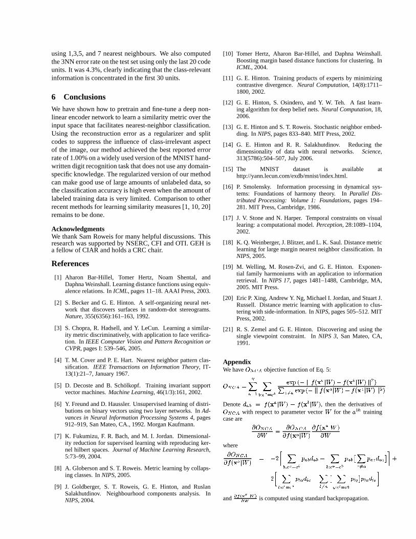
Figure 1: After learning a non-linear transformation from imagesto 30-dimensional code vectors, the Euclidean distance betweencode vectors can be used to measure the similarity between im-ages.

Generalizing this idea to networks with multi-dimensional,real-valued outputs is difficult because the true mutual in-formation depends on the entropy of the output vectors andthis is hard to estimate efficiently for multi-dimensionaloutputs. Approximating the entropy by the log determi-nant of a multidimensional Gaussian works well for learn-ing linear transformations [7], because a linear transforma-tion cannot alter how Gaussian a distribution is. But it doesnot work well for learning non-linear transformations [21]because the optimization cheats by making the Gaussianapproximation to the entropy as bad as possible. The mu-tual information is the difference between the individual en-tropies and the joint entropy, so it can be made to appearvery large by learning individual output distributions thatresemble a hairball. When approximated by a Gaussian, alarge hairball has a large determinant but its true entropy isvery low because the density is concentrated into the hairsrather than filling the space.

The structure in an iid set of image pairs can be decom-posed into the structure in the whole iid set of individualimages, ignoring the pairings, plus the additional struc-ture in the way they are paired. If we focus on model-ing only the additional structure in the pairings, we canfinesse the problem of estimating the entropy of a multi-dimensional distribution. The additional structure can bemodeled by finding a non-linear transformation of each im-age into a low-dimensional code such that paired imageshave codes that are much more similar than images that arenot paired. Adopting a probabilistic approach, we can de-fine a probability distribution over all possible pairs of im-ages, ��� � ��� by using the squared distances between theircodes, � ��� � ��� � ����� � :

� ��� � � � � � � � � � ����� � $ � ����� � � � ������� � � � ����� $ � ���

�� � � � (2)

We can then learn the non-linear transformation by maxi-mizing the log probability of the pairs that actually occur inthe training set. The normalizing term in Eq. 2 is quadraticin the number of training cases rather than exponential inthe number of pixels or the number of code dimensions be-cause we are only attempting to model the structure in thepairings, not the structure in the individual images or themutual information between the code vectors.

The idea of using Eq. 2 to train a multilayer neural net-work was originally described in [9]. They showed thata network would extract a two-dimensional code that ex-plicitly represented the size and orientation of a face if itwas trained on pairs of face images that had the same sizeand orientation but were otherwise very different. Attemptsto extract more elaborate properties were less successfulpartly because of the difficulty of training multilayer neu-ral networks with many hidden layers, and partly becausethe amount of information in the pairings of images isless than � ���� bits per pair. This means that a very largenumber of pairs is required to train a large number of pa-rameters.

Chopra et.al. [3] have recently used a non-probabilistic ver-sion of the same approach to learn a similarity metric forfaces that assigns high similarity to very different images ofthe same person and low similarity to quite similar imagesof different people. They achieve the same effect as Eq.2 by using a carefully hand-crafted penalty function thatuses both positive (similar) and negative (dissimilar) exam-ples. They greatly reduce the number of parameters to belearned by using a convolutional multilayer neural networkand achieve impressive results on a face verification task.

We have recently discovered a very effective and entirelyunsupervised way of training a multi-layer, non-linear ”en-coder” network that transforms the input data vector � intoa low-dimensional feature representation � ��� � ��� that cap-tures a lot of the structure in the input data [14]. This un-supervised algorithm can be used as a pretraining stage toinitialize the parameter vector � that defines the mappingfrom input vectors to their low-dimensional representation.After the initial pretraining, the parameters can be fine-tuned by performing gradient descent in the Neighbour-hood Component Analysis (NCA) objective function intro-duced by [9]. The learning results in a non-linear trans-formation of the input space which has been optimized tomake KNN perform well in the low-dimensional featurespace. Using this nonlinear NCA algorithm to map MNISTdigits into the 30-dimensional feature space, we achieve anerror rate of 1.08%. Support Vector Machines have a sig-nificantly higher error rate of 1.4% on the same version ofthe MNIST task [5].

In the next section we briefly review Neighborhood Com-ponents Analysis and generalize it to its nonlinear counter-part. In section 3, we show how one can efficiently per-

form pretraining to extract useful features from binary orreal-valued data. In section 4 we show that nonlinear NCAsignificantly outperforms linear methods on the MNISTdataset of handwritten digits. In section 5 we show hownonlinear NCA can be regularized by adding an extra termto the objective function. The extra term is the error inreconstructing the data from the code. Using this regular-izing term, we show how nonlinear NCA can benefit fromadditional, unlabeled data. We further demonstrate the su-periority of regularized nonlinear NCA when only smallfraction of the images are labeled.

2 Learning Nonlinear NCAWe are given a set of labeled training cases ����� ��� � � ,� � � ��� ������ � , where � � �� � , and � � ��� � ��� ������ ����� .For each training vector � � , define the probability that point� selects one of its neighbours � (as in [9, 13]) in the trans-formed feature space as:

� �"� � ����� � $�� �"� ������� � ����� � $�� � � � �� �"� � � (3)

We focus on the Euclidean distance metric:

� � � �"! � ��� � � ��� $ � ��� � � ����! �and � �$# � ��� is a multi-layer neural network parametrizedby the weight vector � (see fig 1). The probability thatpoint � belongs to class % depends on the relative proximityof all other data points that belong to class % :

� � � � � % � �'&�)( *)+ � �

� �"� (4)

The NCA objective (as in [9]) is to maximize the expectednumber of correctly classified points on the training data:

,.-0/21 �-&� �43 &�5( *)6 � * +

� �"� (5)

One could alternatively maximize the sum of the log prob-abilities of correct classification:

,.798 �-&� �:3 � ���<; &�5( * 6 � * +

� �"�>= (6)

When � ��� � ��� � � � is constrained to be a linear trans-formation, we get linear NCA. When � ��� � ��� is definedby a multilayer, non-linear neural network, we can explorea much richer class of transformations by backpropagatingthe derivatives of the objective functions in Eq. 5 or 6 withrespect to parameter vector � through the layers of theencoder network. In our experiments, the NCA objective, -?/41

of Eq. 5 worked slightly better than, 798

. We sus-pect that this is because

, -0/21is more robust to handling

outliers., 798

, on the other hand, would strongly penalizeconfigurations where a point in the feature space does notlie close to any other member of its class. The derivativesof Eq. 5 are given in the appendix.

h

W

BinaryVisible Data

BinaryHidden Features

x

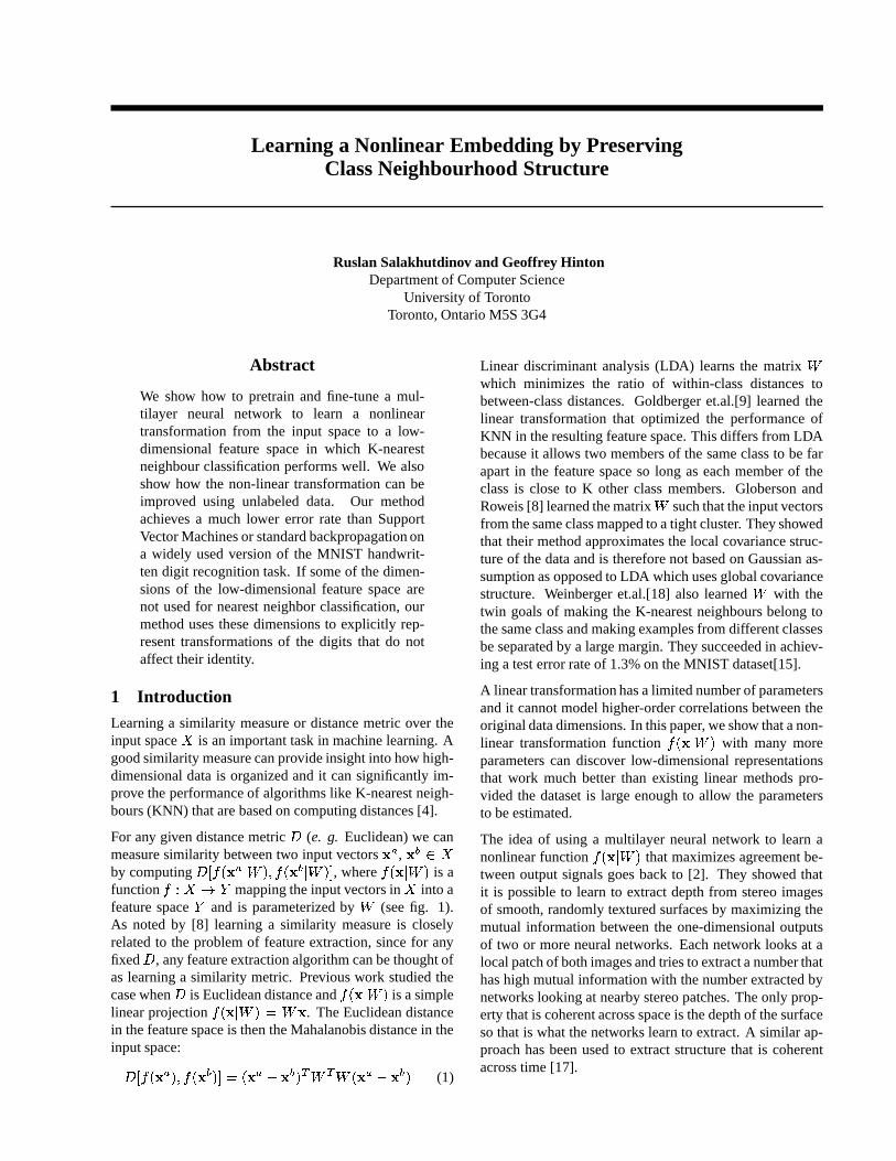
Figure 2: A Restricted Boltzmann Machine. The top layer repre-sents a vector of stochastic binary features @ and and the bottomlayer represents a vector of stochastic binary “visible” variablesA . When modeling real-valued visible variables, the bottom layeris composed of linear units with Gaussian noise.

3 Pretraining

In this section we describe an unsupervised way to learnan adaptive, multi-layer, non-linear ”encoder” network thattransforms the input data vector � into its low-dimensionalfeature representation � ��� � ��� . This learning is treated as apretraining stage that discovers good low-dimensional rep-resentations. Subsequent fine-tuning of the weight vector� is carried out using the objective function in Eq. 5

3.1 Modeling Binary Data

We model binary data (e.g. the MNIST digits) using aRestricted Boltzmann Machine [6, 16, 11] (see fig. 2).The “visible” stochastic binary input vector � and “hidden”stochastic binary feature vector B are modeled by productsof conditional Bernoulli distributions:

� �DC�E � � � � � � F �G��E?H &JI � I E�K I � (7)

� �LK I � � � B � � F �G� I H & E �I EMCNE � (8)

where F �PO � � �MQ � � HSRUT � � is the logistic function, �I E is

a symmetric interaction term between input V and feature W ,and � I , ��E are biases. The biases are part of the overall pa-rameter vector, � . The marginal distribution over visiblevector � is:

� ��� � ��&�X �Y��� � $�Z ��� � B �&���[�\ ] �Y�N� � $�Z �P^ ��_ � � (9)

where Z ��� � B � is an energy term (i.e. a negative log prob-ability + an unknown constant offset) given by:

Z ��� � B � � $ & I � I K I $ & E � E C E $ & I \ E KI C E � I E (10)

The parameter updates required to perform gradient ascentin the log-likelihood can be obtained from Eq. 9:

` � I E � aNb � � � � ��� �b � I E �ca �$d.K I C Efe � ��g�� $ dhK I C E�e�ikj �ml � �

W

W

W +ε

W +ε

W +ε

W +ε

W +ε

W +ε

W +ε

W +ε

W +ε

W +ε

W +ε

W +ε

W +ε

W +ε

W +ε

W +ε

W

W

2

1

500

500

500

500

2000

2000

500

500

2000

2000

500

500

2 2

3 3

1 1

4 4

4T

5

3T

6

2T

7

1T

8

500

500

2000

2000

500

500

2 2

3 3

1 1

4 4

4T

5

3T

6

2T

7

1T

8

RBM

Pretraining

RBM

3

4

30

RBMTop

RBM

3030

Fine−tuning

Encoder

Decoder

�*NCA

����� �����

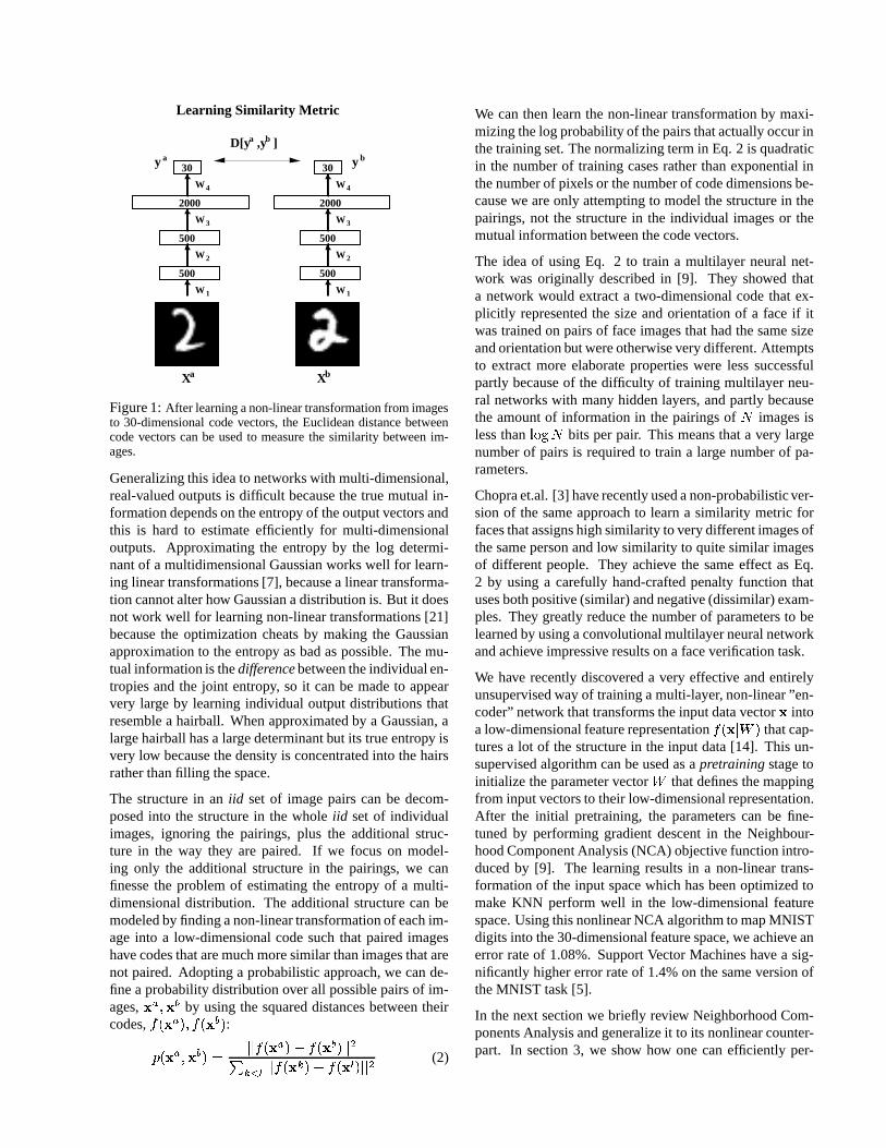
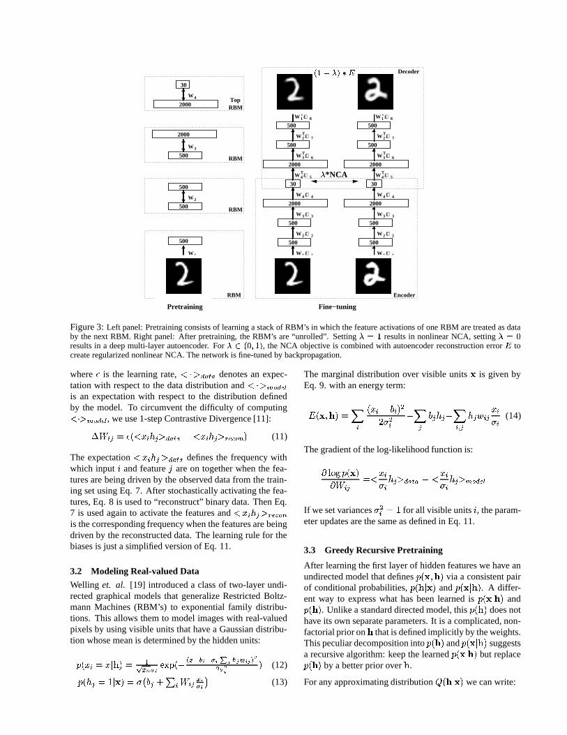
Figure 3: Left panel: Pretraining consists of learning a stack of RBM’s in which the feature activations of one RBM are treated as databy the next RBM. Right panel: After pretraining, the RBM’s are “unrolled”. Setting

� � �results in nonlinear NCA, setting

�����results in a deep multi-layer autoencoder. For

��� � ��� � �, the NCA objective is combined with autoencoder reconstruction error

to

create regularized nonlinear NCA. The network is fine-tuned by backpropagation.

where a is the learning rate, d # e � ��g�� denotes an expec-tation with respect to the data distribution and d # e.i0j �ml �is an expectation with respect to the distribution definedby the model. To circumvent the difficulty of computingd<# e�ikj �ml � , we use 1-step Contrastive Divergence [11]:` � I E �ca � dhK I C�E e � ��g�� $ dhK I C�E e�� l * j�� � (11)

The expectation d K I C�E e � ��g�� defines the frequency withwhich input V and feature W are on together when the fea-tures are being driven by the observed data from the train-ing set using Eq. 7. After stochastically activating the fea-tures, Eq. 8 is used to “reconstruct” binary data. Then Eq.7 is used again to activate the features and d K I C E e � l * j��is the corresponding frequency when the features are beingdriven by the reconstructed data. The learning rule for thebiases is just a simplified version of Eq. 11.

3.2 Modeling Real-valued Data

Welling et. al. [19] introduced a class of two-layer undi-rected graphical models that generalize Restricted Boltz-mann Machines (RBM’s) to exponential family distribu-tions. This allows them to model images with real-valuedpixels by using visible units that have a Gaussian distribu-tion whose mean is determined by the hidden units:

� �LK I � K � B � � 3� ������� ����� � $� "! T � � T ���$#&%(' %�) � %�*,+�-� +� � (12)

� �DC�E � � � � � ��F ;G��E H � I � I E ! ��.� = (13)

The marginal distribution over visible units � is given byEq. 9. with an energy term:

Z ��� � B � � & I �PK I $ � I � ���F �I $ & E ��E�C�E $ & I \ E CNE0/I E K IF I (14)

The gradient of the log-likelihood function is:

b � ��� � ��� �b � I E � d K IF I CNE e � ��g�� $ d KIF I CNE e i0j �ml �

If we set variances F �I � � for all visible units V , the param-eter updates are the same as defined in Eq. 11.

3.3 Greedy Recursive Pretraining

After learning the first layer of hidden features we have anundirected model that defines � ��� � B � via a consistent pairof conditional probabilities, � �DB � � � and � ��� � B � . A differ-ent way to express what has been learned is � ��� � B � and� �DB � . Unlike a standard directed model, this � �PB � does nothave its own separate parameters. It is a complicated, non-factorial prior on B that is defined implicitly by the weights.This peculiar decomposition into � �PB � and � ��� � B � suggestsa recursive algorithm: keep the learned � ��� � B � but replace� �DB � by a better prior over B .

For any approximating distribution 1 �PB � � � we can write:

� ��� � ��� ��� & X 1 �PB � � � � ��� � �PB � H � � � � ��� � B � �$ & X 1 �DB � � � � ��� 1 �PB � � � (15)

If we set 1 �PB � � � to be the true posterior distribution,� �DB � � � (Eq. 7), the bound becomes tight. By freezingthe parameter vector � at the value ����������� (Eq. 7,8)we freeze � ��� � B � , and if we continue to use � %��� ������ tocompute the distribution over B given � we also freeze1 �DB � � � � %��������� � . When � �PB � is implicitly defined by����������� , 1 �DB � � � � %��������� � is the true posterior, but whena better distribution is learned for � �PB � , 1 �DB � � � � %���������� � isonly an approximation to the true posterior. Nevertheless,the loss caused by using an approximate posterior is lessthan the gain caused by using a better model for � �DB � , pro-vided this better model is learned by optimizing the vari-ational bound in Eq. 15. Maximizing this bound with �frozen at ����� ������ is equivalent to maximizing:

& X 1 �DB � � � �'%��������� � � ��� � �PB �This amounts to maximizing the probability of a set of Bvectors that are sampled with probability 1 �PB � � � � %���������� � ,i.e. it amounts to treating the hidden activity vectors pro-duced by applying � %��������� to the real data as if they weredata for the next stage of learning.1 Provided the numberof features per layer does not decrease, [12] showed thateach extra layer increases the variational lower bound inEq. 15 on the log probability of data. This bound does notapply if the layers get smaller, as they do in an encoder,but, as shown in [14], the pretraining algorithm still worksvery well as a way to initialize a subsequent stage of fine-tuning. The pretraining finds a point that lies in a goodregion of parameter space and the myopic fine-tuning thenperforms a local gradient search that finds a nearby pointthat is considerably better.

After learning the first layer of features, a second layer islearned by treating the activation probabilities of the exist-ing features, when they are being driven by real data, as thedata for the second-level binary RBM (see fig. 3). To sup-press noise in the learning signal, we use the real-valuedactivation probabilities for the visible units of every RBM,but to prevent each hidden unit from transmitting more thanone bit of information from the data to its reconstruction,the pretraining always uses stochastic binary values for thehidden units.

The hidden units of the top RBM are modeled with stochas-tic real-valued states sampled from a Gaussian whose meanis determined by the input from that RBM’s logistic visible

1We can initialize the new model of the average conditionalposterior over @ by simply using the existing learned model butwith the roles of the hidden and visible units reversed. This en-sures that our new model starts with exactly the same � � @ � as ourold one.

units. This allows the low-dimensional codes to make gooduse of continuous variables and also facilitates comparisonswith linear NCA. The conditional distributions are given inEq. 12,13, with roles of B and � reversed. Throughout allof our experiments we set variances F �E � � for all hiddenunits W , which simplifies learning. The parameter updatesin this case are the same as defined in Eq. 11.

This greedy, layer-by-layer training can be repeated sev-eral times to learn a deep, hierarchical model in which eachlayer of features captures strong high-order correlations be-tween the activities of features in the layer below.

Recursive Learning of Deep Generative Model:

1. Learn the parameters ��� of a Bernoulli or Gaussianmodel.

2. Freeze the parameters of the lower-level model and usethe activation probabilities of the binary features, whenthey are being driven by training data, as the data fortraining the next layer of binary features.

3. Freeze the parameters ��� that define the 2 ��� layer offeatures and use the activation probabilities of thosefeatures as data for training the 3 ��� layer of features.

4. Proceed recursively for as many layers as desired.

3.4 Details of the training

To speed-up the pretraining, we subdivided the MNISTdataset into small mini-batches, each containing 100 cases,and updated the weights after each mini-batch. Each layerwas greedily pretrained for 50 passes (epochs) through theentire training dataset.2 For fine-tuning model parametersusing the NCA objective function we used the method ofconjugate gradients3 on larger mini-batches of 5000 withthree line searches performed for each mini-batch in eachepoch. To determine an adequate number of epochs andavoid overfitting, we fine-tuned on a fraction of the train-ing data and tested performance on the remaining valida-tion data. We then repeated the fine-tuning on the entiretraining dataset for 50 epochs.

We also experimented with various values for the learningrate, momentum, and weight-decay parameters used in thepretraining. Our results are fairly robust to variations inthese parameters and also to variations in the number oflayers and the number of units in each layer. The preciseweights found by the pretraining do not matter as long as itfinds a good region from which to start the fine-tuning.

4 Experimental ResultsIn this section we present experimental results for theMNIST handwritten digit dataset. The MNIST dataset [15]

2The weights were updated using a learning rate of 0.1, mo-mentum of 0.9, and a weight decay of

��� �.����� �weight

�learning

rate. The weights were initialized with small random values sam-pled from a zero-mean normal distribution with variance 0.01.

3Code is available athttp://www.kyb.tuebingen.mpg.de/bs/people/carl/code/minimize/

1 3 5 7

0.6

0.8

1

1.2

1.4

1.6

1.8

2

2.2

2.4

2.6

2.8

3

3.2

Number of Nearest Neighbours

Tes

t E

rro

r (%

)

Nonlinear NCA 30DLinear NCA 30DAutoencoder 30DPCA 30D

1

23

4

56

7

89

0

Linear NCA LDA PCA

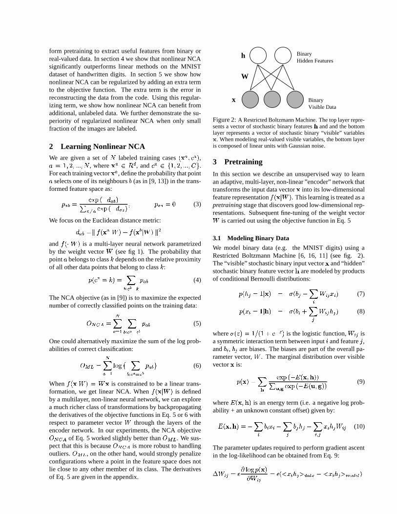
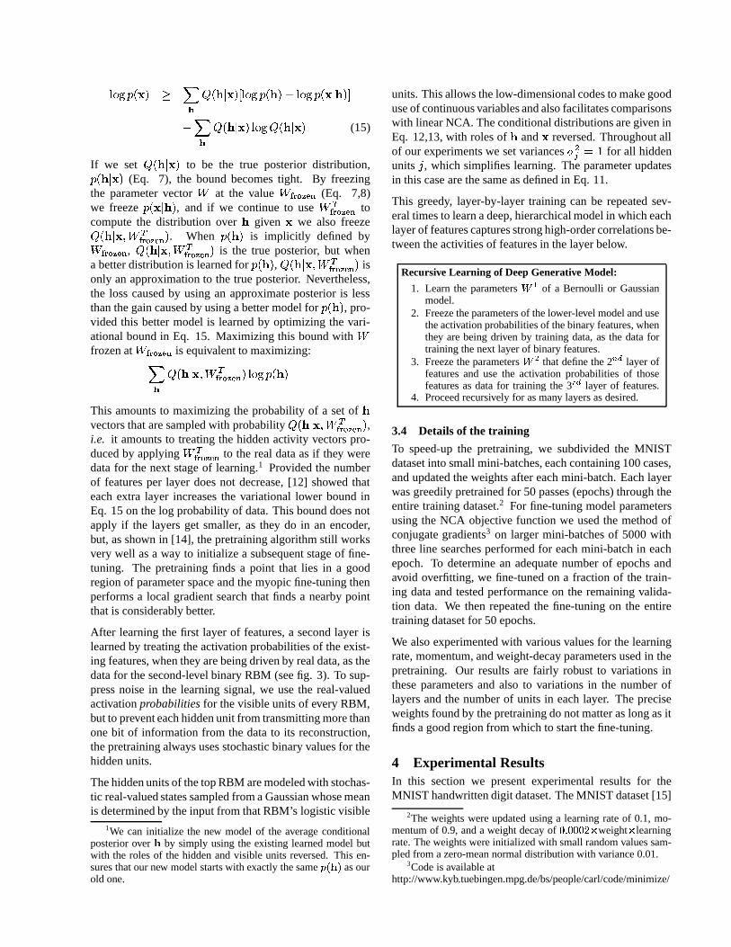
Figure 4: The top left panel shows KNN results on the MNIST test set. The top right panel shows the 2-dimensional codes producedby nonlinear NCA on the test data using a 784-500-500-2000-2 encoder. The bottom panels show the 2-dimensional codes produced bylinear NCA, Linear Discriminant Analysis, and PCA.

contains 60,000 training and 10,000 test images of ����� ���handwritten digits. Out of 60,000 training images, 10,000were used for validation. The original pixel intensities werenormalized to lie in the interval ��� � � and had a preponder-ance of extreme values.

We used a 28 � 28 $ 500 $ 500 $ 2000 $ 30 architecture asshown as fig. 3, similar to one used in [12]. The 30 codeunits were linear and the remaining hidden units were lo-gistic. Figure 4 shows that Nonlinear NCA, after 50 epochsof training, achieves an error rate of 1.08%, 1.00%, 1.03%,and 1.01% using 1,3,5, and 7 nearest neighbours. Thisis compared to the best reported error rates (without us-ing any domain-specific knowledge) of 1.6% for randomlyinitialized backpropagation and 1.4% for Support VectorMachines [5]. Linear methods such as linear NCA orPCA are much worse than nonlinear NCA. Figure 4 (rightpanel) shows the 2-dimensional codes produced by non-linear NCA compared to linear NCA, Linear DiscriminantAnalysis, and PCA.

5 Regularized Nonlinear NCAIn many application domains, a large supply of unlabeleddata is readily available but the amount of labeled data,

which can be expensive to obtain, is very limited so non-linear NCA may suffer from overfitting.

After the pretraining stage, the individual RBM’s at eachlevel can be “unrolled” as shown in figure 3 to create adeep autoencoder. If the stochastic activities of the binaryfeatures are replaced by deterministic, real-valued proba-bilities, we can then backpropagate through the entire net-work to fine-tune the weights for optimal reconstruction ofthe data. Training such deep autoencoders, which does notrequire any labeled data, produces low-dimensional codesthat are good at reconstructing the input data vectors, andtend to preserve class neighbourhood structure [14].

The NCA objective, that encourages codes to lie close toother codes belonging to the same class, can be combinedwith the autoencoder objective function (see fig. 3) to max-imize: �'��� , -0/21 H � � $ � � � $ E � (16)

where, -0/41

is defined in Eq. 5, Z is the reconstructionerror, and � is a trade-off parameter. When the derivativeof the reconstruction error Z is backpropagated throughthe autoencoder, it is combined, at the code level, with thederivatives of

,.-0/21.

1 3 5 7 8

9

10

11

12

13

14

15

16

17

18

19

20

21

Number of Nearest Neighbours

Tes

t E

rro

r (%

)

Regularized NCA (λ=0.99)Nonlinear NCA 30D (λ=1)Linear NCA 30DAutoencoder 30D (λ=0)KNN in pixel space

1 3 5 7 2.5

3

3.5

4

4.5

5

5.5

6

6.5

7

7.5

8

Number of Nearest Neighbours

Tes

t E

rro

r (%

)

Regularized NCA (λ=0.99)Nonlinear NCA 30D (λ=1)Linear NCA 30DAutoencoder 30D (λ=0)KNN in pixel space

1 3 5 7 2

2.5

3

3.5

4

4.5

5

5.5

6

Number of Nearest Neighbours

Tes

t E

rro

r (%

)

Regularized NCA (λ=0.999)Nonlinear NCA 30D (λ=1)Linear NCA 30DAutoencoder 30D (λ=0)KNN in pixel space

1% labels 5% labels 10% labels

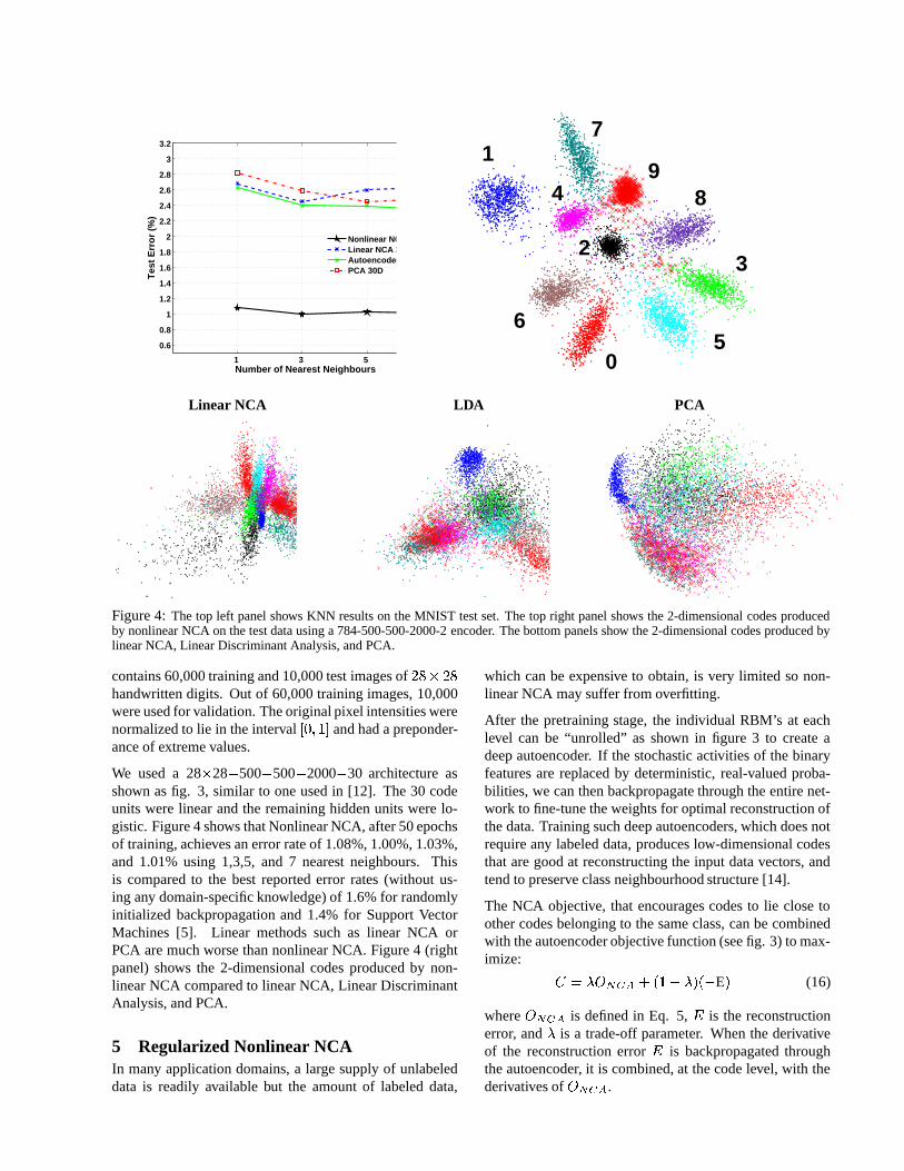
Figure 5: KNN on the MNIST test set when only a small fraction of class labels is available. Linear NCA and KNN in pixel space donot take advantage of the unlabeled data.

30 20 30 20

.......

.......

.......

....... �*NCA

����� �����

Figure 6: Left panel: The NCA objective function is only applied to the first 30code units, but all 50 units are used for image reconstruction. Right panel: Thetop row shows the reconstructed images as we vary the activation of code unit25 from 1 to -23 with a stepsize of 4. The bottom row shows the reconstructedimages as we vary code unit 42 from 1 to -23.

This setting is particularly useful for semi-supervisedlearning tasks. Consider having a set of � labeled train-ing data ���

���� � � , where as before �

�� � , and � � �� � �>���Y���� �>��� , and a set of �� unlabeled training data � � .

Let � � H �� . The overall objective to maximize canbe written as:, � � � �

- �& � �43 &� � * � � *)+� � � H � � $ � �

�

-&� �43 $�Z � (17)

where Z � is the reconstruction error for the input data vec-tor K � . For the MNIST dataset we use the cross-entropyerror:

Z�� � $ & I K �I � �����K �I $ & I � � $ K �I � � ��� � � $ �K �I � (18)

where K �I � � � � � is the intensity of pixel V for the trainingexample � , and �K �I is the intensity of its reconstruction.

When the number of labeled example is small, regular-ized nonlinear NCA performs better than nonlinear NCA( � � � ), which uses the unlabeled data for pretraining butignores it during the fine-tuning. It also performs betterthan an autoencoder ( � � � ), which ignores the labeledset. To test the effect of the regularization when most ofthe data is unlabeled, we randomly sampled 1%, 5% and10% of the handwritten digits in each class and treatedthem as labeled data. The remaining digits were treated

as unlabeled data. Figure 5 reveals that regularized non-linear NCA( � � � � �� )4 outperforms both nonlinear NCA( � � � ) and an autoencoder ( � � � ). Even when the en-tire training set is labeled, regularized NCA still performsslightly better.

5.1 Splitting codes into class-relevant andclass-irrelevant parts

To allow accurate reconstruction of a digit image, the codemust contain information about aspects of the image suchas its orientation, slant, size and stroke thickness that arenot relevant to its classification. These irrelevant aspects in-evitably contribute to the Euclidean distance between codesand harm classification. To diminish this unwanted effect,we used 50-dimensional codes but only used the first 30dimensions in the NCA objective function. The remaining20 dimensions were free to code all those aspects of an im-age that do not affect its class label but are important forreconstruction.

Figure 6 shows how the reconstruction is affected bychanging the activity level of a single code unit. Chang-ing a unit among the first 30 changes the class; changing aunit among the last 20 does not. With � � �J� �� the splitcodes achieve an error rate of 1.00% 0.97% 0.98% 0.97%

4The parameter�

was selected, using cross-validation, fromamong the values � ��� ����� � ������ � ������ � � �� .

using 1,3,5, and 7 nearest neighbours. We also computedthe 3NN error rate on the test set using only the last 20 codeunits. It was 4.3%, clearly indicating that the class-relevantinformation is concentrated in the first 30 units.

6 ConclusionsWe have shown how to pretrain and fine-tune a deep non-linear encoder network to learn a similarity metric over theinput space that facilitates nearest-neighbor classification.Using the reconstruction error as a regularizer and splitcodes to suppress the influence of class-irrelevant aspectof the image, our method achieved the best reported errorrate of 1.00% on a widely used version of the MNIST hand-written digit recognition task that does not use any domain-specific knowledge. The regularized version of our methodcan make good use of large amounts of unlabeled data, sothe classification accuracy is high even when the amount oflabeled training data is very limited. Comparison to otherrecent methods for learning similarity measures [1, 10, 20]remains to be done.

AcknowledgmentsWe thank Sam Roweis for many helpful discussions. Thisresearch was supported by NSERC, CFI and OTI. GEH isa fellow of CIAR and holds a CRC chair.

References

[1] Aharon Bar-Hillel, Tomer Hertz, Noam Shental, andDaphna Weinshall. Learning distance functions using equiv-alence relations. In ICML, pages 11–18. AAAI Press, 2003.

[2] S. Becker and G. E. Hinton. A self-organizing neural net-work that discovers surfaces in random-dot stereograms.Nature, 355(6356):161–163, 1992.

[3] S. Chopra, R. Hadsell, and Y. LeCun. Learning a similar-ity metric discriminatively, with application to face verifica-tion. In IEEE Computer Vision and Pattern Recognition orCVPR, pages I: 539–546, 2005.

[4] T. M. Cover and P. E. Hart. Nearest neighbor pattern clas-sification. IEEE Transactions on Information Theory, IT-13(1):21–7, January 1967.

[5] D. Decoste and B. Scholkopf. Training invariant supportvector machines. Machine Learning, 46(1/3):161, 2002.

[6] Y. Freund and D. Haussler. Unsupervised learning of distri-butions on binary vectors using two layer networks. In Ad-vances in Neural Information Processing Systems 4, pages912–919, San Mateo, CA., 1992. Morgan Kaufmann.

[7] K. Fukumizu, F. R. Bach, and M. I. Jordan. Dimensional-ity reduction for supervised learning with reproducing ker-nel hilbert spaces. Journal of Machine Learning Research,5:73–99, 2004.

[8] A. Globerson and S. T. Roweis. Metric learning by collaps-ing classes. In NIPS, 2005.

[9] J. Goldberger, S. T. Roweis, G. E. Hinton, and RuslanSalakhutdinov. Neighbourhood components analysis. InNIPS, 2004.

[10] Tomer Hertz, Aharon Bar-Hillel, and Daphna Weinshall.Boosting margin based distance functions for clustering. InICML, 2004.

[11] G. E. Hinton. Training products of experts by minimizingcontrastive divergence. Neural Computation, 14(8):1711–1800, 2002.

[12] G. E. Hinton, S. Osindero, and Y. W. Teh. A fast learn-ing algorithm for deep belief nets. Neural Computation, 18,2006.

[13] G. E. Hinton and S. T. Roweis. Stochastic neighbor embed-ding. In NIPS, pages 833–840. MIT Press, 2002.

[14] G. E. Hinton and R. R. Salakhutdinov. Reducing thedimensionality of data with neural networks. Science,313(5786):504–507, July 2006.

[15] The MNIST dataset is available athttp://yann.lecun.com/exdb/mnist/index.html.

[16] P. Smolensky. Information processing in dynamical sys-tems: Foundations of harmony theory. In Parallel Dis-tributed Processing: Volume 1: Foundations, pages 194–281. MIT Press, Cambridge, 1986.

[17] J. V. Stone and N. Harper. Temporal constraints on visuallearing: a computational model. Perception, 28:1089–1104,2002.

[18] K. Q. Weinberger, J. Blitzer, and L. K. Saul. Distance metriclearning for large margin nearest neighbor classification. InNIPS, 2005.

[19] M. Welling, M. Rosen-Zvi, and G. E. Hinton. Exponen-tial family harmoniums with an application to informationretrieval. In NIPS 17, pages 1481–1488, Cambridge, MA,2005. MIT Press.

[20] Eric P. Xing, Andrew Y. Ng, Michael I. Jordan, and Stuart J.Russell. Distance metric learning with application to clus-tering with side-information. In NIPS, pages 505–512. MITPress, 2002.

[21] R. S. Zemel and G. E. Hinton. Discovering and using thesingle viewpoint constraint. In NIPS 3, San Mateo, CA,1991.

AppendixWe have ������� objective function of Eq. 5:

� ����� � ��� � �� � 6 � � +

����� �������� A �� � � ���� A � � � � � ����! �" ����� ���#�$�� A � � � �%�� A � � � � � � �Denote & � �� A � � � �'�� A � � �

, then the derivatives of� ����� with respect to parameter vector � for the (*),+ trainingcase are - � �����-

��

- � �����- �� A � � �- �� A �� � �-

�where- � �����- �� A � � � � � ��. �� � 6 � � + �

& � /� � 6 � � + � 10 �! �� � � & ��24365

��. 78� � � � � 6 �7 & 7 � 7 �" 0 9 � � � � �/: � 7 9 2 � 7 & 7 3

and ;=<=> ? 6A@ BDC; B is computed using standard backpropagation.