LEARMONTH PIPELINE FABRICATION FACILITY SEDIMENT

www.rpsgroup.com/mst

LEARMONTH PIPELINE FABRICATION FACILITY SEDIMENT DISPERSION MODELLING Report

MAW0752J

Learmonth Pipeline

Fabrication Facility Sediment

Dispersion Modelling

Rev 1

27 March 2019

REPORT

MAW0752J | Learmonth Pipeline Fabrication Facility Sediment Dispersion Modelling | Rev 1 | 27 March 2019

www.rpsgroup.com/mst Page ii

Document status

Version Purpose of document Authored by Reviewed by Approved by Review date

Rev A Internal review N. Page D. Wright D. Wright 19/03/2019

Rev 0 Client review N. Page D. Wright D. Wright 22/03/2019

Rev 1 Client review N. Page R. Alexander

D. Wright D. Wright 27/03/2019

Approval for issue

David Wright 27 March 2019

This report was prepared by RPS within the terms of RPS’ engagement with its client and in direct response

to a scope of services. This report is supplied for the sole and specific purpose for use by RPS’ client. The

report does not account for any changes relating the subject matter of the report, or any legislative or

regulatory changes that have occurred since the report was produced and that may affect the report. RPS

does not accept any responsibility or liability for loss whatsoever to any third party caused by, related to or

arising out of any use or reliance on the report.

Prepared by: Prepared for:

RPS MBS Environmental

David Wright

Manager - Perth

Spencer Shute

Principal Environmental Scientist

Level 2, 27-31 Troode Street

West Perth WA 6005

4 Cook Street

West Perth WA 6005

T +61 8 9211 1111

E [email protected]

T +61 9 9226 3166

E [email protected]

REPORT


www.rpsgroup.com/mst Page iii

Contents

1 INTRODUCTION ................................................................................................................................ 1

1.1 Background .............................................................................................................................. 1

1.2 Modelling Scope ....................................................................................................................... 3

2 HYDRODYNAMIC AND WAVE MODELLING .................................................................................. 4

2.1 Overview .................................................................................................................................. 4

2.2 Hydrodynamic Model (D-FLOW) .............................................................................................. 4

2.2.1 Model Description ....................................................................................................... 4

2.2.2 Bathymetry and Domain Definition ............................................................................. 5

2.2.3 Boundary and Initial Conditions .................................................................................. 8

2.2.4 Model Validation ......................................................................................................... 8

2.3 Wave Model (D-WAVE) ......................................................................................................... 15

2.3.1 Model Description ..................................................................................................... 15

2.3.2 Model Implementation .............................................................................................. 15

2.3.3 Model Validation ....................................................................................................... 15

3 SUMMARY OF CHAIN TOW FIELD EXPERIMENT ....................................................................... 18

3.1 Background ............................................................................................................................ 18

3.2 Continuous Turbidity Loggers ................................................................................................ 20

3.3 Vertical Turbidity Profile Data................................................................................................. 20

3.4 Particle Size Distribution Data................................................................................................ 20

3.5 Water Sample TSS and Turbidity Data .................................................................................. 21

4 SEDIMENT FATE MODELLING ...................................................................................................... 23

4.1 General Approach .................................................................................................................. 23

4.2 Model Description .................................................................................................................. 23

4.3 Model Limitations ................................................................................................................... 25

4.4 Model Domain and Bathymetry .............................................................................................. 26

4.5 Pipeline Bundle Tow Project Description and Model Operational Assumptions .................... 28

4.5.1 Overview ................................................................................................................... 28

4.5.2 Bundle Design and Tow Method............................................................................... 28

4.6 Model Sediment Sources ....................................................................................................... 29

4.6.1 Overview ................................................................................................................... 29

4.6.2 Representation of A Single Chain Source ................................................................ 29

4.6.3 Representation of Multiple Chain Sources ............................................................... 31

4.6.4 Scenario Summary ................................................................................................... 31

4.7 Validation of DREDGEMAP Inputs ........................................................................................ 31

5 ENVIRONMENTAL THRESHOLD ANALYSIS ............................................................................... 34

5.1 Overview ................................................................................................................................ 34

5.2 Baseline Water Quality ........................................................................................................... 34

5.3 Marine Fauna: Zone of Impact to Fish ................................................................................... 34

5.4 Marine Environmental Quality ................................................................................................ 35

5.4.1 Overview ................................................................................................................... 35

5.4.2 Ecosystem Health ..................................................................................................... 35

5.4.3 Aesthetic Quality ....................................................................................................... 35

6 RESULTS OF SEDIMENT FATE MODELLING .............................................................................. 36

6.1 Spatial Distributions of TSS ................................................................................................... 36

6.1.1 Flood-Tide Commencement Scenario ...................................................................... 37

6.1.2 Ebb-Tide Commencement Scenario ........................................................................ 49

6.2 Predictions of Management Zone Extents ............................................................................. 61

6.2.1 Flood-Tide Commencement Scenario ...................................................................... 62

6.2.2 Ebb-Tide Commencement Scenario ........................................................................ 64

REPORT


www.rpsgroup.com/mst Page iv

7 REFERENCES ................................................................................................................................. 66

REPORT


www.rpsgroup.com/mst Page v

Tables

Table 3.1 Measured suspended sediment PSDs (MBS, 2018a). .......................................................... 21

Table 3.2 Measured seabed sediment PSDs (MBS, 2018a). ................................................................ 21

Table 4.1 Material size classes used in SSFATE. ................................................................................. 24

Table 4.2 Assumed PSDs of sediments lost to the water column as bundle chains are dragged

across the seabed along the tow route. ................................................................................. 30

Table 4.3 Assumed initial vertical distribution of sediments lost to the water column as bundle

chains are dragged across the seabed along the tow route. ................................................. 30

REPORT


www.rpsgroup.com/mst Page vi

Figures

Figure 1.1 Locations of the proposed Learmonth Pipeline Fabrication Facility project envelope, tow

route and bundle laydown area, and the measurement points of the chain tow field

experiment discussed in Section 3. ......................................................................................... 2

Figure 2.1 Model grid setup showing the domain-decomposition scheme applied, highlighting the

two outermost grids. ................................................................................................................. 6

Figure 2.2 Model grid setup showing the domain-decomposition scheme applied, highlighting the

innermost grid. The locations of the measurement stations (‘Launchway’ and ‘Parking’)

used for model validation are indicated. .................................................................................. 7

Figure 2.3 Comparison of tidal amplitudes from the D-FLOW hydrodynamic model (y-axis) with

those from the XTide database (x-axis) at eight stations located within the model domain. ... 9

Figure 2.4 Time series comparisons of water elevations predicted by the D-FLOW hydrodynamic

model (blue line) with those predicted by the XTide database (green line) over the

validation period of January 2017 at two selected station locations. ..................................... 11

Figure 2.5 Time series comparisons of water elevations predicted by the D-FLOW hydrodynamic

model (blue line) with those predicted by the XTide database (green line) over the

validation period of January 2017 at two selected station locations. ..................................... 12

Figure 2.6 Time series comparisons of modelled and measured depth-averaged currents at the

Launchway ADCP station over the full measurement period (May-June 2018). ................... 13

Figure 2.7 Time series comparisons of modelled and measured depth-averaged currents at the

Parking ADCP station over the full measurement period (May-June 2018). ......................... 14

Figure 2.8 Time series comparisons of modelled and measured wave heights and water levels at the

Launchway ADCP station over the full measurement period (May-June 2018). ................... 17

Figure 3.1 Chain tow tracks and sampling locations (source: MBS, 2018a). .......................................... 19

Figure 3.2 Turbidity logger data. The orange line represents Turbidity Logger 1, north-west of the

tow paths, and the blue line represents Turbidity Logger 2, south-east of the tow paths

(source: MBS, 2018a). ........................................................................................................... 20

Figure 4.1 DREDGEMAP model domain and bathymetry (m MSL). ...................................................... 27

Figure 4.2 Locations of the proposed Learmonth Pipeline Fabrication Facility project envelope, tow

route and laydown area, overlain on existing marine conservation areas. ............................ 28

Figure 4.3 Bundle tow procedure (source: 360 Environmental, 2017c). ................................................. 29

Figure 4.4 Comparison of modelled TSS (converted to turbidity units, NTU) from the final validation

simulation with measured turbidity at the location of Turbidity Logger 2. .............................. 33

Figure 6.1 Predicted 50th percentile depth-averaged TSS throughout the entire flood-tide scenario

duration. ................................................................................................................................. 37


duration. ................................................................................................................................. 38


duration. ................................................................................................................................. 39

Figure 6.4 Predicted 50th percentile maximum TSS throughout the entire flood-tide scenario

duration. ................................................................................................................................. 40


duration. ................................................................................................................................. 41


duration. ................................................................................................................................. 42

Figure 6.7 Predicted 50th percentile bottom concentration throughout the entire flood-tide scenario

duration. ................................................................................................................................. 43


duration. ................................................................................................................................. 44


duration. ................................................................................................................................. 45

Figure 6.10 Predicted 50th percentile bottom thickness throughout the entire flood-tide scenario

duration. ................................................................................................................................. 46

REPORT


www.rpsgroup.com/mst Page vii


duration. ................................................................................................................................. 47


duration. ................................................................................................................................. 48

Figure 6.13 Predicted 50th percentile depth-averaged TSS throughout the entire ebb-tide scenario

duration. ................................................................................................................................. 49


duration. ................................................................................................................................. 50


duration. ................................................................................................................................. 51

Figure 6.16 Predicted 50th percentile maximum TSS throughout the entire ebb-tide scenario duration. . 52



Figure 6.19 Predicted 50th percentile bottom concentration throughout the entire ebb-tide scenario

duration. ................................................................................................................................. 55


duration. ................................................................................................................................. 56


duration. ................................................................................................................................. 57

Figure 6.22 Predicted 50th percentile bottom thickness throughout the entire ebb-tide scenario

duration. ................................................................................................................................. 58


duration. ................................................................................................................................. 59


duration. ................................................................................................................................. 60

Figure 6.25 Predicted zone of influence following application of the appropriate MEQ threshold for

ecosystem health (described in Section 5.4) to total (model and background) TSS

throughout the entire flood-tide scenario duration. ................................................................ 62


aesthetic quality (described in Section 5.4) to total (model and background) TSS

throughout the entire flood-tide scenario duration. ................................................................ 63


ecosystem health (described in Section 5.4) to total (model and background) TSS

throughout the entire ebb-tide scenario duration. .................................................................. 64


aesthetic quality (described in Section 5.4) to total (model and background) TSS

throughout the entire ebb-tide scenario duration. .................................................................. 65

REPORT


www.rpsgroup.com/mst Page 1

1 INTRODUCTION

1.1 Background

Subsea 7 proposes to construct and operate a new pipeline fabrication facility, to be located at Learmonth

adjacent to the south-western shoreline of Exmouth Gulf in Western Australia, approximately 35 km south of

the Exmouth townsite. The Learmonth Pipeline Fabrication Facility will build pipeline bundles for the offshore

oil and gas industry and may produce an average of 1-2 bundles per year (and a maximum of 3 per year). The

bundles will be constructed onshore before being launched via a launchway crossing the beach and towed

offshore along a predetermined route (Figure 1.1). As the bundle moves beyond the end of the launchway,

chains suspended beneath the bundle will be in contact with the seabed, causing a disturbance of

unconsolidated material and potential suspension of sediments into the water column.

During the environmental assessment process for the Learmonth Pipeline Fabrication Facility, the potential

severity, extent and persistence of suspended sediment plumes associated with the bundle launch and tow

operation was identified as requiring analysis to determine the potential impacts to water quality or benthic

communities and habitat (BCH). RPS was commissioned by MBS Environmental (MBS), on behalf of Subsea

7, to undertake sediment dispersion modelling of the pipeline bundle launch and tow operation to aid

assessment of the potential environmental consequences in terms of generation of total suspended sediment

(TSS) concentrations and sedimentation.

This technical report contains a summary of the sediment fate model inputs, methodologies and assumptions,

and the model outcomes following analysis of specified threshold criteria.

REPORT



Figure 1.1 Locations of the proposed Learmonth Pipeline Fabrication Facility project envelope, tow route and bundle laydown area, and the measurement points of the chain tow field experiment discussed in Section 3.

REPORT



1.2 Modelling Scope

The scope of work required to complete the sediment dispersion modelling included the following key tasks:

1. Review of the available current, wave and turbidity field data;

2. Development and validation of a hydrodynamic model, and production of up to one month of

hydrodynamic simulation data;

3. Development and validation of a wave model, and production of up to one month of wave simulation data;

4. Review of the chain tow field experiment and application of the data to determine appropriate inputs to

the sediment dispersion model;

5. Undertaking of sediment dispersion modelling;

6. Post-processing, combination and analysis of simulation outputs to determine outcomes including zones

of impact and influence based on specified threshold criteria.

REPORT



2 HYDRODYNAMIC AND WAVE MODELLING

2.1 Overview

Modelling of the potential sediment dispersion from the pipeline bundle launch activities required temporal and

spatial representation of the hydrodynamic and wave conditions within the project area. A hydrodynamic and

wave model framework for Exmouth Gulf was constructed and validated for this study.

The hydrodynamic and wave modelling for the project was conducted using the Delft3D suite of software. The

Delft3D suite is a fully integrated computer software package composed of several modules (e.g. flow, waves,

sediment, water quality, and ecology) grouped around a common interface. This software suite has been

developed to carry out studies with a multi-disciplinary approach and multi-dimensional calculations (e.g. 2-D

and 3-D) for a range of systems, such as oceanic, coastal, estuarine and river environments. It can simulate

the interaction of flows, waves, sediment transport, morphological developments, water quality and aquatic

ecology. Specific modules of the Delft3D suite are referenced in this report, following the convention of the

software developers, with the suffix D- (e.g. D-FLOW for the Delft3D Hydrodynamics module and D-WAVE for

the Delft3D Spectral Wave module).

The Delft3D suite has been developed by Deltares, an independent institute for applied research on water with

over 30 years of experience in modelling aquatic systems (http://www.deltares.nl/en). The Delft3D suite of

models adheres to the International Association for Hydro-Environment Engineering and Research guidelines

for documenting the validity of computational modelling software, closely replicating an array of analytical,

laboratory, schematic and real-world data.

2.2 Hydrodynamic Model (D-FLOW)

2.2.1 Model Description

To simulate the hydrodynamics within Exmouth Gulf and the surrounding area, a three-dimensional model with

accurate representations of the bathymetry and spatially-varying wind stress was developed. The model

framework was built through the combination of a large-scale regional model with smaller refined regions, or

sub-domains.

The D-FLOW model is ideally suited to represent the hydrodynamics of complex coastal waters, including

regions where the tidal range creates large intertidal zones and where buoyancy processes are important.

RPS has applied the model for numerous studies in the region.

D-FLOW is a multi-dimensional (2-D or 3-D) hydrodynamic (and transport) simulation program which

calculates non-steady flow and transport phenomena that result from tidal, meteorological and baroclinic

forcing on a rectilinear or a curvilinear, boundary-fitted grid. In three-dimensional simulations, the vertical grid

can be defined following the sigma-coordinate approach, where the local water depth is divided into a series

of layers with thickness at a set proportion of the depth.

D-FLOW allows for the establishment of a series of interconnected (two-way, dynamically-nested) curvilinear

grids of varying resolution; a technique referred to as “domain decomposition”. This allows for the generation

of a series of grids with progressively increasing spatial resolution, down to an appropriate scale for accurate

resolution of the hydrodynamics associated with features such as dredged channels. The main advantage of

domain decomposition over traditional one-way, or static, nesting systems is that the model domains interact

seamlessly, allowing transport and feedback between the regions of different scales. The ability to dynamically

couple multiple model domains offers a flexible framework for hydrodynamic model development. This

modelling method was applied in this study.

Inputs to the model, as discussed in the following sections, included:

• Bathymetry of the study area. The wetting and drying of the intertidal zones was simulated in applicable

areas.

http://www.deltares.nl/en

REPORT



• Boundary elevation forcing data.

• Spatially-varying surface wind and pressure data.

2.2.2 Bathymetry and Domain Definition

The hydrodynamic model was established over the domain shown in Figure 2.1 and Figure 2.2. Accurate

bathymetry is a significant factor in development of a model framework required to resolve highly variable wave

and current conditions. The bathymetry was developed using data from the C-MAP electronic chart database

and supplemented with data from Geoscience Australia where relevant and required.

The composite bathymetric data was interpolated onto the D-FLOW Cartesian grid. The resultant bathymetry

is shown in Figure 2.1 and Figure 2.2. The extent and shape of the model coastline will change as water levels

rise and fall with tidal movements due to the inclusion of wetting and drying within the model system.

The vertical grid of the model comprised three layers of varying thickness, depending on location, throughout

the domain. Three layers was found to be enough to resolve the circulation and provide suitable bed level

currents, without overly compromising model performance. As the model was set up as a proportional sigma-

grid in the vertical dimension, these layers therefore represented a terrain-following arrangement with a layer

thickness of 33.3% of the total local water depth.

To offset the computational effort required for a large, multi-layered model domain, and to achieve adequate

horizontal and temporal resolution, a multiple-grid (domain-decomposition) strategy was applied using two

sub-domains of varying horizontal grid cell size (Figure 2.1 and Figure 2.2). Horizontal resolutions within each

sub-domain were 250 m for the main operational area (sub-grid 2), 600 m for the Exmouth Gulf intermediate

region (sub-grid 1) and 2 km for the outer domain (sub-grid 0).

Each sub-domain is an individual hydrodynamic model simulated in parallel with the others, with dynamic

coupling at the shared boundaries between sub-domains. The outermost sub-domain captured large-scale

oceanographic phenomena which progressively fed into the finer-resolution domains representing the area of

interest. The resolution of the innermost sub-domain was specified after assessment of the requirement to

adequately resolve the variation in current fields, and in turn the sediment dynamics.

REPORT



Figure 2.1 Model grid setup showing the domain-decomposition scheme applied, highlighting the two outermost grids.

REPORT



Figure 2.2 Model grid setup showing the domain-decomposition scheme applied, highlighting the innermost grid. The locations of the measurement stations (‘Launchway’ and ‘Parking’) used for model validation are indicated.

REPORT



2.2.3 Boundary and Initial Conditions

2.2.3.1 Overview

As the hydrodynamics in the study area are controlled primarily by tidal flows and wind forcing, these processes

were explicitly included in the developed model.

The model was forced on the open boundaries of the outer sub-domain with time series of water elevation

obtained for the chosen simulation period. Spatially-varying wind speed and wind direction data was used to

force the model across the entire domain.

2.2.3.2 Water Elevation

Water elevations at hourly intervals were obtained from the TPXO8.0 database, which is the most recent

iteration of a global model of ocean tides derived from measurements of sea-surface topography by the

TOPEX/Poseidon satellite-borne radar altimeters. Tides are provided as complex amplitudes of earth-relative

sea-surface elevation for eight primary (M2, S2, N2, K2, K1, O1, P1, Q1), two long-period (Mf, Mm) and three non-

linear (M4, MS4, MN4) harmonic constituents at a spatial resolution of 0.25°.

The tidal sea level data was augmented with non-tidal sea level elevation data from the global Hybrid

Coordinate Ocean Model (HYCOM; Bleck, 2002; Chassignet et al., 2003; Halliwell, 2004), created by the

USA’s National Ocean Partnership Program (NOPP) as part of the Global Ocean Data Assimilation Experiment

(GODAE). The HYCOM model is a three-dimensional model that assimilates observations of sea surface

temperature, sea surface salinity and surface height, obtained by satellite instrumentation, along with

atmospheric forcing conditions from atmospheric models to predict drift currents generated by such forces as

wind shear, density, sea height variations and the rotation of the Earth.

The HYCOM model is configured to combine the three vertical coordinate types currently in use in ocean

models: depth (z-levels), density (isopycnal layers), and terrain-following (σ-levels). HYCOM uses isopycnal

layers in the open, stratified ocean, but uses the layered continuity equation to make a dynamically smooth

transition to a terrain-following coordinate in shallow coastal regions, and to z-level coordinates in the mixed

layer and/or unstratified seas. Thus, this hybrid coordinate system allows for the extension of the geographic

range of applicability to shallow coastal seas and unstratified parts of the world ocean. It maintains the

significant advantages of an isopycnal model in stratified regions while allowing more vertical resolution near

the surface and in shallow coastal areas, hence providing a better representation of the upper ocean physics

than non-hybrid models. The model has global coverage with a horizontal resolution of 1/12th of a degree

(~7 km at mid-latitudes) and a temporal resolution of 24 hours.

2.2.3.3 Wind Forcing

Spatially-variable wind data was sourced from the Australian Digital Forecast Database (ADFD), which

contains official weather forecast elements produced by the Bureau of Meteorology (BoM) – such as

temperature, rainfall and weather types – presented in a gridded format. The ADFD data was selected for the

study site because it includes the influence of localised sea-breezes and topographic features such as North

West Cape. The ADFD data has a horizontal resolution of 1/20th of a degree and a temporal resolution of 1

hour.

2.2.4 Model Validation

2.2.4.1 Comparison of Modelled and Measured Water Elevation

Validation of the water level changes predicted by the D-FLOW hydrodynamic model configuration was

provided through comparisons to independent predictions from the XTide tidal constituent database (Flater,

1998). Comparison of model tidal amplitudes with the XTide database showed strong agreement (Figure 2.3).

Time series comparisons for four tide stations situated at locations near Exmouth also showed good agreement

(Figure 2.4 and Figure 2.5).

REPORT



In general, a consistent match is observed between water elevations calculated by the D-FLOW model and

those predicted by XTide (Figure 2.4). Both the amplitude and phase of the semidiurnal tidal signal are clearly

reproduced at each station, as is the timing of the spring-neap cycle. The D-FLOW model slightly overpredicts

high tides and underpredicts low tides, which indicates there was a small difference between the datums used

to compare these different data sets rather than actual amplitude differences.

Figure 2.3 Comparison of tidal amplitudes from the D-FLOW hydrodynamic model (y-axis) with those from the XTide database (x-axis) at eight stations located within the model domain.

2.2.4.2 Comparison of Modelled and Measured Currents

Validation of the model-predicted currents was conducted for a spring/neap tide period during May and June

2018 by comparing the model results to measured data (GHD, 2018). Measured current velocity data was

collected at an inshore station (‘Launchway’; 22.206° S, 114.170° E; water depth ~14 m) and an offshore

station (‘Parking’; 21.980° S, 114.309° E; water depth ~20 m), as indicated in Figure 2.2.

The comparison of depth-averaged currents at the Launchway station showed strong agreement between

measured and modelled data with respect to current speed and directional components (Figure 2.6). The

comparison of depth averaged currents at the Parking station also showed strong agreement with respect to

current speed (Figure 2.7), with the east-west component of current speed slightly underestimated. The strong

harmonic component of the current velocity at both stations indicates the dominance of tidal forcing.

REPORT



To provide quantitative statistical measures of the hydrodynamic model performance, the Index of Agreement

(IOA: Willmott, 1981; Willmott et al., 1985) and the Mean Absolute Error (MAE: Willmott, 1982; Willmott &

Matsuura, 2005) were calculated for each ADCP station.

The IOA is a standardised measure of the degree of model prediction error and varies between 0 (complete

disagreement between predictions and observations) and 1 (perfect agreement). Although it is difficult to find

guidelines for what values of the IOA might represent a good agreement, Willmott et al. (1985) suggests that

values meaningfully larger than 0.5 represent good model performance. The MAE is simply the average of the

absolute values of the differences between the modelled and measured values. MAE is a more natural

measure of average error (Willmott & Matsuura, 2005) and more readily understood. Clearly, the higher the

IOA and the lower the MAE, the better the model performance.

An important point to note regarding both – and in fact most – measures of model performance is that slight

phase differences in the series can result in a seemingly poor statistical comparison, particularly in rapidly

changing series. It is therefore always important to consider both the statistics and the visual representation

of the comparison (Willmott et al., 1985).

Other traditional error estimates, such as the correlation coefficient (R) and the root mean square error (RMSE)

are problematic and prone to ambiguities and bias (Willmott, 1982; Willmott & Matsuura, 2005). Consequently,

they are not reported in isolation here.

Table 2.1 summarises the R, IOA, RMSE and MAE values for both ADCP locations, and demonstrates the

high quality of the hydrodynamic model performance.

Table 2.1 Statistical comparisons of modelled and measured depth-averaged currents at the Launchway and Parking ADCP stations over the full measurement period (May-June 2018).

Station Parameter Correlation

Coefficient (R) Index of

Agreement (IOA)

Root-Mean-Square Error

(RMSE)

Mean Absolute Error (MAE)

Launchway ADCP Magnitude 0.9171 0.9517 0.04 m/s 0.03 m/s

Direction 0.9327 0.9653 39.17° 16.76°

Parking ADCP Magnitude 0.9574 0.9574 0.06 m/s 0.05 m/s

Direction 0.9646 0.9731 33.88° 22.76°

REPORT



Figure 2.4 Time series comparisons of water elevations predicted by the D-FLOW hydrodynamic model (blue line) with those predicted by the XTide database (green line) over the validation period of January 2017 at two selected station locations.

REPORT



Figure 2.5 Time series comparisons of water elevations predicted by the D-FLOW hydrodynamic model (blue line) with those predicted by the XTide database (green line) over the validation period of January 2017 at two selected station locations.

REPORT



Figure 2.6 Time series comparisons of modelled and measured depth-averaged currents at the Launchway ADCP station over the full measurement period (May-June 2018).

REPORT



Figure 2.7 Time series comparisons of modelled and measured depth-averaged currents at the Parking ADCP station over the full measurement period (May-June 2018).

REPORT



2.3 Wave Model (D-WAVE)

2.3.1 Model Description

Reliable forecasting for the fate of fine sediments in the study location, which is a wave-influenced coastal

region, required the input of wave spectra information to calculate the shear-stress and orbital velocities

imposed by waves which will affect the settlement and re-suspension of fine material that is initially suspended

by the bundle tow operation. D-WAVE is a variant of the well-known SWAN wave model that has been

customised for compatibility with the Delft3D software suite.

The D-WAVE model is a spectral phase-averaging wave model originally developed by the Delft University of

Technology. D-WAVE, a third-generation model based on the energy balance equation, is a numerical model

for simulating realistic estimates of wave parameters in coastal areas for given wind, bottom and current

conditions.

D-WAVE includes algorithms for the following wave propagation processes: propagation through geographic

space; refraction and shoaling due to bottom and current variations; blocking and reflections by opposing

currents; and transmission through or blockage by obstacles. The model also accounts for dissipation effects

due to white-capping, bottom friction and wave breaking as well as non-linear wave-wave interactions. D-

WAVE is fully spectral (in all directions and frequencies) and computes the evolution of wind waves in coastal

regions with shallow water depths and ambient currents.

RPS has successfully applied D-WAVE in many studies in the region.

2.3.2 Model Implementation

The D-WAVE model was developed to cover the same area defined by the hydrodynamic model (Figure 2.1

and Figure 2.2) but employed a modified sub-gridding scheme within Exmouth Gulf. The outer grid (sub-grid

0) was identical to that shown in Figure 2.1, but the intermediate grid (sub-grid 1) was extended to cover the

main operational area. The bathymetry and wind data input to the wave model was the same as used for the

hydrodynamic model. Time-varying water level information for each grid node in the wave model was provided

by the output of the hydrodynamic model. The boundary data to represent swells imposed from a distance was

sourced from the AUSWAVE-R model, which is a forecast data product produced by Australia’s BoM and

based on an implementation of the third-generation wind-wave modelling framework WaveWatch III operated

by the US National Oceanic and Atmospheric Administration (NOAA). The AUSWAVE-R data has a horizontal

resolution of 1/10th of a degree and a temporal resolution of 1 hour.

2.3.3 Model Validation

Validation of the model-predicted waves was conducted for a spring/neap tide period during May and June

2018 by comparing the model results to measured data (GHD, 2018). Measured wave data was collected at

the inshore station (‘Launchway’; 22.206° S, 114.170° E; water depth ~14 m) indicated in Figure 2.2.

The comparison showed good agreement between measured and modelled data, with significant wave heights

typically less than 1 m during the validation period (Figure 2.8). The periods when the modelled and measured

wave heights differ tend to be associated with very low measured wave energy. Overprediction of low wave

energy will be conservative with respect to predictions of sediment fate. The water levels measured at the

Launchway station were in strong agreement with the model-predicted water levels (Figure 2.8).

To provide quantitative statistical measures of the wave model performance, the R, IOA, RMSE and MAE

values were calculated for the ADCP station in a similar manner to the validation of the hydrodynamic model

currents, as described in Section 2.2.4.2.

Table 2.2 summarises the R, IOA, RMSE and MAE values for the ADCP location, and demonstrates the high

quality of the wave model performance.

REPORT



Table 2.2 Statistical comparisons of modelled and measured wave heights at the Launchway ADCP station over the full measurement period (May-June 2018).

Station Parameter Correlation

Coefficient (R) Index of

Agreement (IOA)

Root-Mean-Square Error

(RMSE)

Mean Absolute Error (MAE)

Launchway ADCP

Significant Wave

Height 0.5958 0.7505 0.22 m 0.17 m

Peak Direction 0.5529 0.7327 89.10° 66.79°

REPORT



Figure 2.8 Time series comparisons of modelled and measured wave heights and water levels at the Launchway ADCP station over the full measurement period (May-June 2018).

REPORT



3 SUMMARY OF CHAIN TOW FIELD EXPERIMENT

3.1 Background

The major unknown factors with respect to modelling sediment dispersion related to the pipeline bundle launch

and tow operation were the specification of suitable sediment source terms. These terms include the flux rate,

particle size distribution (PSD) and vertical distribution of suspended sediments that are likely to be generated

by the chains disturbing the local seabed environment. Modifications to the source terms are the greatest

drivers of changes in plume dispersion patterns, influencing the amount of sediment released to the water

column and the relative rates of settlement and resuspension. Therefore, it was highly important that these

source terms were accurately defined in the sediment dispersion model.

A field experiment involving the towing of one chain along the seabed was conducted along a nearshore

section of the tow route offshore Heron Point in Exmouth Gulf, to help define the source terms for input to the

model.

A total of three tows were completed during the experiment on the morning of 7th November 2018, running in

a north-east to south-west direction, commencing during a flood tide and ending at slack water high tide. The

measurements included:

• Two continuous turbidity loggers placed 100 m to the north-west and south-east of the chain tow path at

an elevation of 1 m above the seabed;

• Multiple vertical turbidity profiles adjacent to the tow paths;

• Multiple near-seabed water samples for on-vessel TSS analysis or laboratory-based analysis of turbidity

and PSDs;

• Benthic grab samples of sediment in the vicinity of the tow paths for laboratory-based analysis of PSDs.

The chain tow tracks and sampling locations are presented in Figure 3.1. More detail regarding the methods

and data collected during the experiment is contained in MBS (2018a). This section contains a review of the

field data that is relevant to: (i) definition of the sediment source terms designed to be representative of each

bundle chain; and (ii) validation of the model inputs.

REPORT



Figure 3.1 Chain tow tracks and sampling locations (source: MBS, 2018a).

REPORT



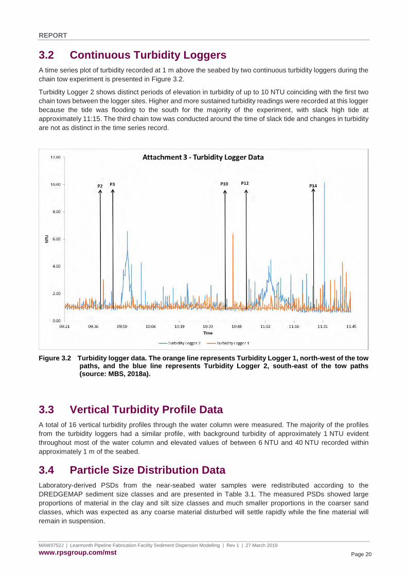
3.2 Continuous Turbidity Loggers

A time series plot of turbidity recorded at 1 m above the seabed by two continuous turbidity loggers during the

chain tow experiment is presented in Figure 3.2.

Turbidity Logger 2 shows distinct periods of elevation in turbidity of up to 10 NTU coinciding with the first two

chain tows between the logger sites. Higher and more sustained turbidity readings were recorded at this logger

because the tide was flooding to the south for the majority of the experiment, with slack high tide at

approximately 11:15. The third chain tow was conducted around the time of slack tide and changes in turbidity

are not as distinct in the time series record.

Figure 3.2 Turbidity logger data. The orange line represents Turbidity Logger 1, north-west of the tow paths, and the blue line represents Turbidity Logger 2, south-east of the tow paths (source: MBS, 2018a).

3.3 Vertical Turbidity Profile Data

A total of 16 vertical turbidity profiles through the water column were measured. The majority of the profiles

from the turbidity loggers had a similar profile, with background turbidity of approximately 1 NTU evident

throughout most of the water column and elevated values of between 6 NTU and 40 NTU recorded within

approximately 1 m of the seabed.

3.4 Particle Size Distribution Data

Laboratory-derived PSDs from the near-seabed water samples were redistributed according to the

DREDGEMAP sediment size classes and are presented in Table 3.1. The measured PSDs showed large

proportions of material in the clay and silt size classes and much smaller proportions in the coarser sand

classes, which was expected as any coarse material disturbed will settle rapidly while the fine material will

remain in suspension.

REPORT



Laboratory-derived PSDs from the benthic sediment samples, modified to suit the DREDGEMAP size classes,

are presented in Table 3.2. The measured PSDs revealed that in situ sediments near the chain tow tracks

have a large proportion of material sizes classed as fine sand or larger (~54%), although there are also

significant proportions of clay and silt material (~46%). It should be noted that the PSDs of the in situ sediments

are significantly different from the in-water PSDs, revealing the rapid settlement of coarser material in the water

column.

Table 3.1 Measured suspended sediment PSDs (MBS, 2018a).

Sediment Grain Size Class

Size Range (µm)

PSD (%) P7

PSD (%) P8

PSD (%) P11

PSD (%) P12

PSD (%) P14-2

PSD (%) P16

Clay <7 45.1 35.2 43.5 39.2 43.0 39.9

Fine Silt 8-34 39.7 39.3 39.9 37.9 36.7 37.0

Coarse Silt 35-74 13.5 19.9 13.8 17.0 15.1 17.6

Fine Sand 75-130 1.8 5.5 2.9 5.9 5.0 5.5

Coarse Sand >130 0.0 0.0 0.0 0.1 0.1 0.0

Table 3.2 Measured seabed sediment PSDs (MBS, 2018a).

Sediment Grain Size Class

Size Range (µm)

PSD (%) P17

PSD (%) P12-2

Clay <7 12.6 14.8

Fine Silt 8-34 15.7 17.9

Coarse Silt 35-74 16.2 14.9

Fine Sand 75-130 16.5 13.7

Coarse Sand >130 39.0 38.7

3.5 Water Sample TSS and Turbidity Data

Table 3.3 presents a summary of the on-vessel TSS and laboratory-derived turbidity measurements for the

near-seabed water samples. The measurements show that TSS in the near-seabed layer ranged between

2 mg/L and 30 mg/L during the experimental period, with turbidity ranging up to 52 NTU.

The five locations where both TSS and turbidity were measured were used to determine a relationship between

TSS and turbidity at the site. The relationship was found to be: TSS (mg/L) = 1.75 * Turbidity (NTU).

This relationship is site-specific and was required for the validation of DREDGEMAP model source term inputs,

because the TSS model outputs needed to be related to the field measurements of turbidity.

REPORT



Table 3.3 Measured TSS and turbidity (MBS, 2018a).

Site ID TSS (mg/L) Turbidity (NTU)

P1 8.0 -

P4 2.0 -

P7 20.0 12.0

P8 8.0 3.6

P10 14.0 -

P11 19.0 14.0

P12 30.0 16.0

P13 5.0 -

P14 5.0 -

P14-2 - 52.0

P16 26.0 16.0

REPORT



4 SEDIMENT FATE MODELLING

4.1 General Approach

Estimates for the three-dimensional distribution of sediments suspended during the pipeline bundle tow

operation have been derived for the full duration of the activities using numerical modelling. This modelling

relied upon specification of sediment discharges over time for each of the expected sources of sediment

suspension, and predicted the evolution of the combined sediment plumes via current transport, dispersion,

sinking and sedimentation. The model allowed for the subsequent resuspension of settling sediments due to

the erosive effects of currents and waves. Thus, the fate of sediments was assessed beyond their initial

settling.

Forcing was provided using predictions of three-dimensional current fields and two-dimensional wave fields

for the study area, which are described in Section 2.

4.2 Model Description

Modelling of the dispersion of suspended sediment resulting from the pipeline bundle tow operation was

undertaken using an advanced sediment fate model, Suspended Sediment FATE (SSFATE), operating within

the RPS DREDGEMAP model framework. This model computes the advection, dispersion, differential sinking,

settlement and resuspension of sediment particles. The model can be used to represent inputs from a wide

range of suspension sources, producing predictions of sediment fate both over the short-term (minutes to days

following a discharge source) and longer term (days to years following a discharge source).

SSFATE allows the three-dimensional predictions of suspended sediment concentrations and seabed

sedimentation to be assessed against allowable exposure thresholds. Sedimentation thresholds often relate

to burial depths or rates, while suspended sediment concentration thresholds are usually more complicated,

involving tiered exposure duration and intensities. As a result, assessing the project-generated sediment

distributions against these thresholds in both three-dimensional space and time is a computationally intensive

task. A variety of suspended sediment concentration threshold formulations have recently been applied in

Western Australian coastal waters and at present there are no general guidelines.

SSFATE is a computer model originally developed jointly by the US Army Corps of Engineers (USACE)

Engineer Research and Development Center (ERDC) and RPS to estimate suspended sediment

concentrations generated in the water column and deposition patterns generated due to dredging operations

in a current-dominated environment, such as a river (Johnson et al., 2000; Swanson et al., 2000, 2004). RPS

has significantly enhanced the capability of SSFATE to allow the prediction of sediment fate in marine and

coastal environments where wave forcing becomes important for reworking the distribution of sediments

(Swanson et al., 2007).

SSFATE is formulated to simulate far-field effects (~25 m or larger scale) in which the mean transport and

turbulence associated with ambient currents are dominant over the initial turbulence generated at the

discharge point. A five-class particle-based model predicts the transport and dispersion of the suspended

material. The classes include the 0-130 µm range of sediment grain sizes that typically result in plumes.

Heavier sediments tend to settle very rapidly, remain more stable over time and are not relevant over the

longer durations (>1 hour) and larger spatial scales (>25 m) of interest here. Table 4.1 shows the standard

material classes used in SSFATE for suspended sediment.

REPORT



Table 4.1 Material size classes used in SSFATE.

Material Class Description Particle Size Range (µm)

Clay <7

Fine Silt 8-34

Coarse Silt 35-74

Fine Sand 75-130

Coarse Sand >130

Particle advection is calculated using three-dimensional current fields, obtained from hydrodynamic modelling,

thus the model can account for vertical changes in the currents within the water column. For example, as

particles sink towards the seabed they will tend to be moved at slower speeds due to the slowing of currents

by friction at the seabed. Particle diffusion is assumed to follow a random walk process using a Lagrangian

approach of calculating transport, which uses a grid-less space to remove limitations of grid resolution,

artefacts due to grid boundaries, and also maintain a high degree of mass conservation.

Following release into the model space, the sediment cloud evolves according to the following processes:

• Advection due to the three-dimensional current field.

• Diffusion by a random walk model with the mass diffusion rate specified, ideally, from measurements at

the site. As particles represent an ensemble of real particles, each particle in the model has an associated

Gaussian distribution governed by particle age and the mass diffusion properties of the surrounding water.

• Settlement or sinking of the sediment due to buoyancy forces. Settlement rates are determined from the

particle class sizes and include allowance for flocculation and other concentration-dependent behaviour,

following the model of Teeter (2000).

• Potential deposition to the seabed determined using a model that couples the deposition across particle

classes (Teeter, 2000). The likelihood and rate of deposition depends on the shear stress at the seabed.

High shear inhibits deposition, and in some cases excludes it altogether with sediment remaining in

suspension. The model allows for partial deposition of individual particles according to a practical

deposition rate, thereby allowing the bulk sediment mass to be represented by fewer particles.

• Potential resuspension from the seabed, if previously deposited, at a rate governed by exceedance of a

shear stress threshold at the seabed due to the combined action of waves and currents. Different

thresholds are applied for resuspension depending upon the size of the particle and the duration of

sedimentation, based on empirical studies that have demonstrated that newly-settled sediments will have

higher water content and are more easily resuspended by lower shear stresses (Swanson et al., 2007).

The resuspension flux calculation also accounts for armouring of fine particles within the interstitial spaces

of larger particles. Thus, the model can indicate whether deposits will stabilise or continue to erode over

time given the shear forces that occur at the site. Resuspended material is released back into the water

column to be affected by the processes defined above.

SSFATE formulations and proof of performance have been documented in a series of USACE Dredging

Operations and Environmental Research (DOER) Program technical notes (Johnson et al., 2000; Swanson et

al., 2000), and published in the peer-reviewed literature (Andersen et al., 2001; Swanson et al., 2004; Swanson

et al., 2007). SSFATE has been applied and validated by RPS against observations of sedimentation and

suspended sediments at multiple locations in Australia, notably Cockburn Sound for Fremantle Ports and

Mermaid Sound for the Pluto dredging project.

REPORT



4.3 Model Limitations

There are inherent limitations to the accuracy of numerical models. The possible sources of uncertainty within

the modelling conducted for the sediment fate assessment of the Learmonth Pipeline Fabrication Facility tow

operation include:

• The equations and algorithms applied in the model. The formulations included in the model, as discussed

in Section 4.2, were selected to achieve the best possible representation of the relevant processes and

have been proven to be valid over a range of projects.

• The accuracy of the physical (current and wave) inputs to the model. Current and wave forcing inputs

were provided from validated three-dimensional hydrodynamic and wave models created and customised

for the study area. The accuracy of these models is suitable, as good correlations with field measurements

and independent model predictions have been achieved, with the uncertainties minimised and

quantifiable. The hydrodynamic and wave models are described in Section 2. It should be noted that the

model inputs are a hindcast of past metocean conditions; the overall trends reflected in this data will be

broadly reflected in future conditions, but conditions on any given day during an actual tow operation may

be quite different.

• The accuracy of pipeline bundle tow methodology inputs to the model. Specification of the proposed

bundle tow methodologies was provided by MBS after consultation with Subsea 7. Any assumptions made

to achieve a realistic representation of the bundle tow activities are outlined in Section 4.5 and were based

on extensive past project experience in the modelling of sediment dispersion from sediment-disturbing

operations in the marine environment.

• The accuracy of the material properties input to the model. Data relating to sediments in situ on the seabed

and suspended in the water column was obtained during a baseline water and sediment quality

assessment (360 Environmental, 2017a) and a chain tow field trial (MBS, 2018a), with the latter discussed

in Section 3. From this data, the properties of the in situ material on the seabed and how it may be

distributed in the water column are reasonably well known for the nearshore area where the experiments

were undertaken. In addition, a BCH survey conducted in the bundle laydown area (360 Environmental,

2017b) found that the sediments there could be characterised as “fine sand with shell grit” and “muddy

fine sand with shell grit”. Although it is not possible to determine with certainty from these data sets how

the material properties will vary between the launchway and the bundle laydown area, an assumption was

made that the PSDs measured during the nearshore chain tow field trial – dominated by clays and fine

silts – were representative of the entire tow route. This is a conservative (worst-case) assumption with

regard to the mobility of material that is released into the water column from the bundle tow operation.

• The accuracy of the sediment source terms input to the model. The source definition in the model is

flexible and can be applied to any sediment source by specifying the time-varying flux rate, PSD and

vertical profile in the water column. This information will be specific to the pipeline bundle design, the tow

methodology and the material encountered at the site, and therefore can only be determined with

confidence from a pilot study at the site or field measurements during deployment of a pipeline bundle.

The chain tow field trial (MBS, 2018a) discussed in Section 3 provided data for sediment disturbance from

the action of a single chain, and this data was used to form assumptions with regard to the behaviour

associated with many chains in sequence. The assumptions are outlined in Section 4.6 and were based

on literature review and extensive past project experience. The trial results provided greater certainty

around the expected levels of sediment resuspension and its behaviour in the water column than is often

the case when commencing a modelling exercise, and as such it is considered likely that the model results

are an accurate representation of the outcomes during a bundle launch and tow operation.

The major sources of uncertainty for the sediment fate modelling are the modelled bundle tow methodology

and sediment source inputs to the model. The assumptions made were based on literature review and

experience, and aimed to give a good representation of the sources of suspended sediment that will result

from the proposed bundle tow operation. However, as there were uncertainties in the inputs to the model, the

results should be considered as indicative of the expected ranges in magnitude and distribution of suspended

sediments and sedimentation, rather than an exact prediction.

REPORT



4.4 Model Domain and Bathymetry

The DREDGEMAP model domain established for the pipeline bundle tow operation extended approximately

53 km north-south by 34 km east-west (Figure 4.1), covering a large proportion of Exmouth Gulf. The model

grid covers the section of the western Exmouth Gulf coastline from just north of the Exmouth townsite to just

south of Point Lefroy. The offshore boundaries of the domain were imposed at a reasonable distance from the

proposed sediment disturbance areas, to allow potential sediment drift patterns in offshore directions to be

adequately captured.

This region lies within the model domain of the Delft3D hydrodynamic and wave models that provide the current

and wave inputs to DREDGEMAP (see Section 2). A grid resolution of 20 m by 20 m was selected to ensure

that existing features in the domain were adequately defined and that the sediment source characteristics

along the tow route were appropriately represented.

REPORT



Figure 4.1 DREDGEMAP model domain and bathymetry (m MSL).

REPORT



4.5 Pipeline Bundle Tow Project Description and Model Operational Assumptions

4.5.1 Overview

Information outlining the proposed pipeline bundle tow operation for the Learmonth Pipeline Fabrication Facility

has been drawn from the Section 38 Referral document (360 Environmental, 2017c), subsequent email

discussions, and input data provided by MBS. The operation to be modelled has been broken into two phases:

• Phase 1: Launch and tow of the pipeline bundle, assumed to be 10 km in length, along the defined route

to the laydown area over a period of approximately 12 hours at a speed of 2 knots;

• Phase 2: A post-operation settlement period of 60 hours.

The launch site, pipeline route and laydown area are located in the western half of Exmouth Gulf (Figure 4.2).

The following sections outline the details of the bundle tow operation and highlights any assumptions that were

made.

Figure 4.2 Locations of the proposed Learmonth Pipeline Fabrication Facility project envelope, tow route and laydown area, overlain on existing marine conservation areas.

4.5.2 Bundle Design and Tow Method

The bundle design assumed for the sediment dispersion modelling was based on the most common design as

specified by MBS and Subsea 7. A pipeline bundle is comprised of a number of pipes contained within a larger

REPORT



pipe casing which is manufactured as one segment up to 10 km long (360 Environmental, 2017c). The chains

that will contact the seabed during the launch are typically located at approximately 20 m intervals along the

length of the bundle; assuming a 10 km bundle length (worst case) means approximately 500 chains may be

expected to contact the seabed. The typical chains used in the bundles are of 76 mm diameter with a link

length of 304 mm.

During a launch, the towhead at the offshore end of the bundle is connected to a tug (the ‘leading tug’) which

slowly (≤2 knots) heads offshore, pulling the bundle along the track and into the ocean until the bundle reaches

sufficient water depth to allow connection to another tug (the ‘trailing tug’; Figure 4.3). As the bundle moves

beyond the end of the launchway, the chains suspended beneath the bundle will be in contact with the seabed.

These chains will potentially remain in contact with the seabed over the section of the proposed tow route out

to the end of the laydown area, a distance of approximately 44 km.

Figure 4.3 Bundle tow procedure (source: 360 Environmental, 2017c).

4.6 Model Sediment Sources

4.6.1 Overview

To accurately represent the bundle tow operation in DREDGEMAP, a range of information was defined for the

proposed operation, including bundle design, tow speed and seabed sediment types (see Section 4.5). It is

evident that each chain will act as a separate source of suspended sediment plumes during towing of the

bundle. However, each of these sources will be identical in strength and persistence, as the chain dimensions

and characteristics will be the same.

In the DREDGEMAP model, each source is defined by specifying the time-varying flux rate, PSD and vertical

profile in the water column. The following sections outline how the provided design information and the field

data from the chain tow experiment has been used to represent the bundle tow operation in the model and

explain any assumptions that have been made to supplement the available information.

4.6.2 Representation of A Single Chain Source

The PSD used in the model to represent the material likely to be resuspended by a chain dragging along the

seabed was based on the PSD of the material found in the water samples collected during the chain tow

experiment (Section 3.4). The PSDs of the water column samples all showed a similar distribution when

redistributed according to the DREDGEMAP sediment grain size classes; therefore, an average PSD of the

samples was applied in the modelling as outlined in Table 4.2.

The vertical profile data collected during the chain tow experiment revealed that the sediment resuspended by

a chain dragging along the seabed remains concentrated close to the seabed, with the majority found in the

bottom 1 m of the water column and only a minimal increase in turbidity above this point (see Section 3.3).

The vertical profile outlined in Table 4.3 was assumed for each chain in the model, based on the field

measurements. This profile places the majority of the material within the lower 1 m of the water column and

distributes progressively smaller proportions up to a maximum elevation of 9.5 m from the seabed. Although

REPORT



the measurements did not show detectable increases in turbidity above an elevation of 1 m from the seabed,

the vertical profile takes into consideration that the profiles were measured a safe distance (~20 m) away from

the source where some of the suspended material will have begun to settle. This assumption is considered

conservative (worst-case) and was validated against the field measurements before being applied to the

model.

Table 4.2 Assumed PSDs of sediments lost to the water column as bundle chains are dragged across the seabed along the tow route.

Sediment Grain Size Class Size Range (µm) PSD (%)

Clay <7 41.0

Fine Silt 8-34 38.0

Coarse Silt 35-74 16.0

Fine Sand 75-130 5.0

Coarse Sand >130 0.0

Table 4.3 Assumed initial vertical distribution of sediments lost to the water column as bundle chains are dragged across the seabed along the tow route.

Elevation Example Elevation (m ASB) – 15 m

Water Depth Vertical Distribution (%) of

Sediments

9.5 m (ASB) 9.5 5.0

5.0 m (ASB) 5.0 10.0

2.0 m (ASB) 2.0 20.0

1.0 m (ASB) 1.0 25.0

0.5 m (ASB) 0.5 40.0

The time-varying flux rate is the most difficult source term to define even with the aid of field experiment data,

as it cannot be directly measured. A method to estimate the volume of material suspended by the dragging of

a chain along the seabed was determined based on experience, and this method was validated by replicating

the chain tow experiment in test model simulations and comparing predicted suspended sediment

concentrations with those of the field experiment. A description of the flux rate calculation method is provided

in this section, with a discussion of the validation process provided in Section 4.7.

The tow route was split into seven sections based on bathymetry, and the number of chain links assumed to

be in contact with the seabed was varied depending on the average depth within each section of the route. In

the innermost section (nearshore), it was assumed that six chain links would usually be in contact; in the

outermost section (including the laydown area), it was assumed that two chain links would be in contact.

The flux rate for one chain was calculated as the volume of material on the seabed likely to be disturbed by

the dragging chain, multiplied by a rate of suspension of this material into the water column. The volume of

material disturbed by each chain link was calculated as the cross-sectional area of contact (width of 274 mm

x diameter of 76 mm), multiplied by the length of the route section under consideration, multiplied further by

the number of chain links in contact with the seabed within the route section. The end result is the total volume

of material expected to be disturbed by a chain. In this way, the disturbed volume is greatest in the shallow

nearshore areas and reduces as the chain moves offshore to deeper waters.

Based on past project experience and the mode of action of the chain, it was assumed that the suspension

rate of the disturbed material will vary from 0.1-1.0% of the disturbed volume. A value of 0.6% was applied to

the chain drag source based on sensitivity analysis during the validation simulations (see Section 4.7).

REPORT



4.6.3 Representation of Multiple Chain Sources

At any moment in time after its initial launch, many chains spaced along the bundle will be touching the seabed.

Each of these chains will produce a potential suspended sediment plume, with the sources being cumulative.

A modelling approach was developed based on the bundle design which allowed a large number of

simultaneous sources to be combined and assessed in a cumulative manner.

To represent the worst-case situation, where the number of chains in contact with the seabed – and therefore

the flux rate – is maximised, a maximum bundle length of 10 km and a minimum chain spacing of 20 m was

assumed. This means that approximately 500 chains will contact the seabed to varying degrees over the

duration of the tow operation. Assuming a maximum tow speed of 2 knots, one chain will be launched every

20 seconds. Because the DREDGEMAP model has a minimum time step of 60 seconds, three chains were

assumed to be launched within every model time step. The calculated flux rate for one chain was multiplied by

three to suit. A total of 166 individual model simulations were run, each following an identical path and

containing identical source characteristics but offset in time from the preceding simulation by 60 seconds. The

operational duration is approximately 12 hours from the first chain entering the water to the last chain entering

the bundle laydown area.

The model output from all simulations was cumulatively summed and analysed to provide a single four-

dimensional time series of spatial TSS concentration and sedimentation representative of the entire pipeline

bundle.

Allowing for the expected low speed of the bundle, and the fact that the chains do not present an unbroken

cross-section to the water as they move, it is not considered likely that the chains will cause any hydrodynamic

effects which act to pull turbid water from the bottom to the sea surface. It is pertinent that no visible plumes

were observed on the surface at any point during the chain tow field trial (MBS, 2018a) and that elevated

turbidity measured above 1 m from the seabed was minimal. This trial replicated the conditions under which

chains will be dragging along the seabed and did so at a speed (3 knots) which is faster than the expected

bundle speed (2 knots).

4.6.4 Scenario Summary

A summary of the scenarios that were modelled is as follows:

• A pipeline bundle launch occurring during a flood tide (the most likely situation);

• A pipeline bundle launch occurring during an ebb tide.

Each scenario comprised 166 separate simulations run over appropriate 3-day periods during January 2017.

This month was selected for modelling because it was deemed to be representative of typical wave conditions

likely to be encountered at a time of year when wind speeds are strongest. The transport of sediment will be

heavily influenced by the tidal state at the time of launch.

4.7 Validation of DREDGEMAP Inputs

Validation of the source terms chosen to represent the chains in the DREDGEMAP model was completed

using data from the chain tow field experiment. The conditions of the trial were replicated in the model, with

sediment released along three line sources defined to match the timing (relative to tidal state) and location of

the three chain tow tracks from the experiment (Figure 3.1).

The simulation utilised the flux rate, source PSD and vertical distribution in the water column as outlined in

Section 4.6.2. Model parameters were tuned to reproduce the TSS concentrations measured in the field. The

time-varying flux rate was the most difficult source term to define, and as such this was used as the main

calibration factor; a range of sensitivity simulations were run with a varying flux rate applied. A flux rate value

of 0.6% was found to achieve the best match with the range of TSS values measured in the experiment.

Table 4.4 presents a comparison of modelled TSS values from the final validation simulation against measured

TSS values. The modelled TSS values were extracted from the simulation at times and locations matching the

REPORT



times and locations of the field samples. The comparisons reveal that the modelled TSS values are not always

accurate for the exact location and time; however, the model adequately reproduces the range and variability

of TSS values found in the measured data.

Figure 4.4 presents a time-series of modelled TSS (converted to turbidity units) from the final validation

simulation at the location of Turbidity Logger 2 compared against the measured turbidity data at this station.

The time series reveals a good match in the timing and magnitude of the elevation in turbidity at the logger

location during the three chain tow trials.

Table 4.4 Comparison of modelled TSS values from the final validation simulation against on-vessel water sample TSS measurement and laboratory turbidity measurements converted to TSS.

Site ID Measured TSS

(On-Vessel) (mg/L) Measured Turbidity (Laboratory) (NTU)

Measured TSS (Converted from Turbidity) (mg/L)

Modelled TSS (mg/L)

P1 8.0 - - 20.0

P4 2.0 - - 18.0

P7 20.0 12.0 21.0 12.0

P8 8.0 3.6 6.3 3.0

P10 14.0 - - 7.0

P11 19.0 14.0 24.5 27.0

P12 30.0 16.0 28.0 24.0

P13 5.0 - - 6.0

P14 5.0 - - 3.0

P16 26.0 16.0 28.0 18.0

REPORT



Figure 4.4 Comparison of modelled TSS (converted to turbidity units, NTU) from the final validation simulation with measured turbidity at the location of Turbidity Logger 2.

REPORT



5 ENVIRONMENTAL THRESHOLD ANALYSIS

5.1 Overview

Predictions of TSS for each scenario were assessed against a series of water quality thresholds to categorise

the modelled outcomes into zones of potential impact and influence, defined with regard to environmental

sensitivities in the study region. These thresholds, and the technical justification which followed guidance from

the WAMSI Dredging Node, were supplied to RPS (MBS, 2018b).

Thresholds for three management zones were defined:

• Zone of impact to fish;

• Zone of influence for ecosystem health;

• Zone of influence for aesthetic quality.

5.2 Baseline Water Quality

In the calculation of thresholds for the Marine Environmental Quality (MEQ) criteria, which are dependent on

the baseline turbidity data, an NTU-TSS relationship of TSS = 1.75*NTU was applied. This conversion factor

was calculated as the average value for the site-specific data samples summarised in MBS (2018a).

Background TSS concentrations were added to the model-predicted TSS concentrations prior to threshold

analysis, and the methodology for each threshold is described in the following sections. Water quality data

collected during November and December 2018 at two sites, KP2 and KP4.5 (MBS, 2018c), was used as a

source of background TSS levels.

Water quality data was also collected during May and June 2018 (GHD, 2018), with average turbidity levels of

4.34 NTU at the launchway and 3.64 NTU at the bundle laydown area. However, the November-December

data (with average turbidity levels of 2.00-4.45 NTU) was considered most representative of background

turbidity during the summer period selected for modelling.

5.3 Marine Fauna: Zone of Impact to Fish

A recent study (Wenger et al., 2018) was undertaken to assess the potential vulnerability of coastal fish and

fisheries to dredging activities on a global scale. The study included the development of threshold reference

values for suspended sediment.

Within an environment which regularly experienced elevated suspended sediment concentrations, such as

Exmouth Gulf, it is likely that the majority of species would have a degree of tolerance to suspended sediment.

Thus, the threshold values necessary to protect 80% of species from physical damage or lethal impacts

(58 mg/L and 274 mg/L, respectively; Wenger et al., 2018) would likely ensure the protection of all local

species. Among all life history stages, there was a clear relationship between suspended sediment

concentration and exposure duration. For example, exposure of larvae to concentrations up to 60 mg/L did not

have a lethal impact until after 24 hours (Wenger et al., 2018).

Calculation of this zone of impact was undertaken by assessing a 24-hour rolling average of depth-averaged

TSS data from the model, with the addition of appropriate background TSS data, against a threshold value of

60 mg/L at every grid cell in the model domain.

The background TSS value applied was the average baseline turbidity measured at the KP4.5 location

(22.240° S, 114.138° E) during the one-month monitoring period (4.45 NTU = 7.79 mg/L). Because the

specified threshold is a fixed value independent of the baseline turbidity data, using the larger KP4.5 baseline

values (relative to KP2) means lower model concentrations are required to trigger the threshold. This is the

most conservative (worst-case) approach.

REPORT



5.4 Marine Environmental Quality

5.4.1 Overview

In 2004, the Department of Environment (DoE) ran a planned and targeted public consultation process to

obtain comment on environmental values, environmental quality objectives, and how they should be applied

geographically within the State marine waters from Exmouth Gulf to Cape Keraudren. The resulting report

(DoE, 2006) recommends the Levels of Ecological Protection (LEPs) from the outlined interim Environmental

Values (EVs) and Environmental Quality Objectives (EQOs) agreed upon during consultation.

For most environmental quality indicators, the approach adopted for comparing monitoring data with the EQOs

and determining when a significant and unacceptable change has occurred is consistent with ANZECC &

ARMCANZ (2000). For physical stressors, such as turbidity or TSS, the approach for high ecological protection

areas (the majority of Exmouth Gulf) is to compare the median of the test-site data (or modelled impact data)

with the 80th percentile of the unimpacted reference distribution (EPA, 2017).

5.4.2 Ecosystem Health

Calculation of this zone of influence was undertaken by assessing a 24-hour rolling median of depth-averaged

TSS data from the model, with the addition of appropriate background TSS data, against a threshold value of

4.10 mg/L at every grid cell in the model domain.

The background TSS value applied was the average baseline turbidity measured at the KP2 location

(22.222° S, 114.154° E) during the one-month monitoring period (2.00 NTU = 3.50 mg/L). Because the

specified threshold is calculated from the baseline turbidity data, using the smaller KP2 baseline values

(relative to KP4.5) means lower model concentrations are required to trigger the threshold. This is the most

conservative (worst-case) approach. The threshold value (80th percentile baseline TSS) was calculated as

4.10 mg/L.

5.4.3 Aesthetic Quality

Calculation of this zone of influence was undertaken by assessing a 24-hour rolling average of depth-averaged

TSS (as a proxy for turbidity) data (from the surface to a depth of 6 m) from the model, with the addition of

appropriate background TSS data, against a threshold value of 4.20 mg/L at every grid cell in the model

domain.

The background TSS value applied was the same as that used for the MEQ ecosystem health threshold. The

threshold value (20% increase in TSS, as a proxy for turbidity, in the top 6 m of the water column) was

calculated as 4.20 mg/L.

REPORT



6 RESULTS OF SEDIMENT FATE MODELLING

6.1 Spatial Distributions of TSS

Simulations indicated that there may be significant spatial patchiness in the distribution of TSS at any point in

time during the pipeline bundle launch and tow operation because of variability in the number of sediment

suspension sources, variability in the flux from each of these sources, and the varying dynamics of the

transport, settlement and resuspension processes affecting the sediments.

The most pronounced differences in the predicted concentrations at any point in time are found in the vertical

distributions, with a distinct increase in concentration towards the seabed. Thus, the spatial area affected

above a given concentration is always greater in the near-seabed layer than in the near-surface layer.

Plume concentrations and distributions are forecast to vary markedly from hour to hour. To explore this

variability, statistical distributions are shown in the following sections for both the flood-tide and ebb-tide launch

scenarios. Percentile distributions will summarise the outcomes over the entire scenario and do not represent

an instantaneous plume footprint at any point in time.

The calculated 50th (or median), 80th and 95th percentile distributions (representing values in the model domain

that will be exceeded 50%, 20% and 5% of the time, respectively) are shown in the following figures for each

scenario:

• Depth-averaged TSS: Figure 6.1 to Figure 6.3 (flood-tide case) and Figure 6.13 to Figure 6.15 (ebb-tide

case).

• Maximum TSS: Figure 6.4 to Figure 6.6 (flood-tide case) and Figure 6.16 to Figure 6.18 (ebb-tide case).

• Bottom concentration: Figure 6.7 to Figure 6.9 (flood-tide case) and Figure 6.19 to Figure 6.21 (ebb-tide

case).

• Bottom thickness: Figure 6.10 to Figure 6.12 (flood-tide case) and Figure 6.22 to Figure 6.24 (ebb-tide

case).

The general pattern observed in each scenario is that material will be suspended in the lower layers of the

water column and will drift to one side of the tow route (depending on the tidal state), before a reasonable

proportion of this material is deposited during the next slack water period. The remaining sediments in the

water column will then be transported back and forth over the tow route, with deposition occurring steadily,

until only very low concentrations (~0.1 mg/L) remain suspended after more than 48 hours. The sediments are

mostly fines and the sinking rates are low, but as the majority of the material is suspended close to the seabed

it is not expected to persist in the water column for extended durations.

The greatest suspended and deposited concentrations are seen in shallower waters, where more chain links

will be in contact with the seabed and the flux rate will be higher than in deeper waters. Once the tow operation

has concluded there is no source of sediment other than wave-induced resuspension of deposited material,

which is negligible due to low wave heights.

Modelling showed that peak TSS concentrations will be encountered during the operation when sediment is

actively being disturbed. The settlement period – when the disturbed sediment settles out and little

resuspension occurs – will see progressively lowered concentrations. Peak TSS concentrations of 100 mg/L

or greater are restricted to the immediate vicinity of the tow route, and due to the nature of the operation these

concentrations will be transient occurrences.

The sedimentation variables indicate settlement and accumulation over time, whereas the water-column

variables reflect the continuous movement of an ever-reducing mass of suspended material once operational

activities have concluded.

REPORT



6.1.1 Flood-Tide Commencement Scenario

6.1.1.1 Depth-Averaged TSS

Figure 6.1 Predicted 50th percentile depth-averaged TSS throughout the entire flood-tide scenario duration.

REPORT




REPORT




REPORT



6.1.1.2 Maximum TSS

Figure 6.4 Predicted 50th percentile maximum TSS throughout the entire flood-tide scenario duration.

REPORT




REPORT




REPORT



6.1.1.3 Bottom Concentration

Figure 6.7 Predicted 50th percentile bottom concentration throughout the entire flood-tide scenario duration.

REPORT




REPORT




REPORT



6.1.1.4 Bottom Thickness

Figure 6.10 Predicted 50th percentile bottom thickness throughout the entire flood-tide scenario duration.

REPORT




REPORT




REPORT



6.1.2 Ebb-Tide Commencement Scenario

6.1.2.1 Depth-Averaged TSS

Figure 6.13 Predicted 50th percentile depth-averaged TSS throughout the entire ebb-tide scenario duration.

REPORT




REPORT




REPORT



6.1.2.2 Maximum TSS

Figure 6.16 Predicted 50th percentile maximum TSS throughout the entire ebb-tide scenario duration.

REPORT




REPORT




REPORT



6.1.2.3 Bottom Concentration

Figure 6.19 Predicted 50th percentile bottom concentration throughout the entire ebb-tide scenario duration.

REPORT




REPORT




REPORT



6.1.2.4 Bottom Thickness

Figure 6.22 Predicted 50th percentile bottom thickness throughout the entire ebb-tide scenario duration.

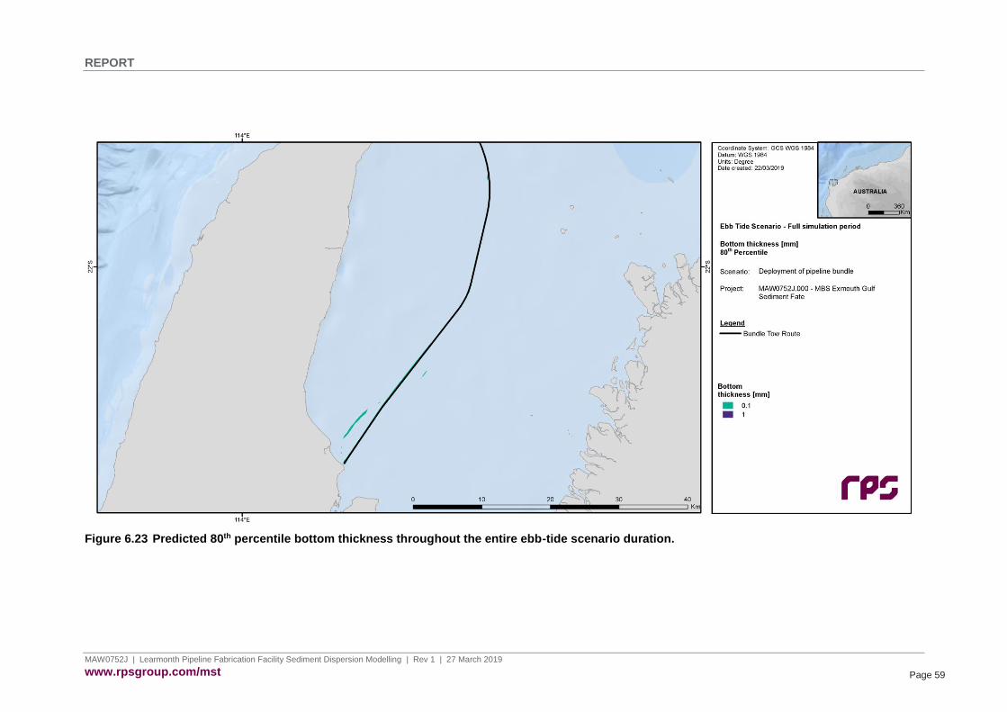
REPORT




REPORT




REPORT



6.2 Predictions of Management Zone Extents

The calculated extents of the defined management zones over the entire bundle launch and tow operation are

shown in the following sections for both the flood-tide and ebb-tide launch scenarios.

In both the flood-tide and ebb-tide launch cases, the threshold associated with the zone of impact to fish is not

forecast to be exceeded at any time. As such, no figures are presented.

Figure 6.25 and Figure 6.27 show the zone of influence associated with the MEQ ecosystem health threshold

for the flood-tide and ebb-tide launch cases, respectively. In both cases, the threshold is forecast to be

exceeded in a zone mainly confined to the shallowest half of the tow route and its surroundings, with the

location of the exceedances dependent on the tidal state at launch time.

Figure 6.26 and Figure 6.28 show the zone of influence associated with the MEQ aesthetic quality threshold

for the flood-tide and ebb-tide launch cases, respectively. In both cases, the threshold is forecast to be

exceeded only in isolated patches near the launch site, with the location of the exceedances dependent on the

tidal state at launch time.

It should be noted that the indicated management zone extents in each case represent a cumulative measure

of exceedances of the relevant thresholds over a 72-hour period, following the threshold criteria described in

Section 5. They do not represent an instantaneous plume footprint at any point in time.

The indicated areas of threshold exceedances are largely a reflection of the areas of sediment confluence due

to the proximity to key activity areas, where there is a sustained input of suspended sediments over periods of

several hours.

REPORT



6.2.1 Flood-Tide Commencement Scenario

6.2.1.1 Marine Environmental Quality: Ecosystem Health

Figure 6.25 Predicted zone of influence following application of the appropriate MEQ threshold for ecosystem health (described in Section 5.4) to total (model and background) TSS throughout the entire flood-tide scenario duration.

REPORT



6.2.1.2 Marine Environmental Quality: Aesthetic Quality

Figure 6.26 Predicted zone of influence following application of the appropriate MEQ threshold for aesthetic quality (described in Section 5.4) to total (model and background) TSS throughout the entire flood-tide scenario duration.

REPORT



6.2.2 Ebb-Tide Commencement Scenario

6.2.2.1 Marine Environmental Quality: Ecosystem Health

Figure 6.27 Predicted zone of influence following application of the appropriate MEQ threshold for ecosystem health (described in Section 5.4) to total (model and background) TSS throughout the entire ebb-tide scenario duration.

REPORT



6.2.2.2 Marine Environmental Quality: Aesthetic Quality

Figure 6.28 Predicted zone of influence following application of the appropriate MEQ threshold for aesthetic quality (described in Section 5.4) to total (model and background) TSS throughout the entire ebb-tide scenario duration.

REPORT



7 REFERENCES 360 Environmental 2017a, Learmonth Bundle Launch Site: Baseline water and sediment quality assessment,

report prepared for Subsea 7 by 360 Environmental Pty Ltd, West Leederville, WA, Australia.

360 Environmental 2017b, Bundle laydown area benthic communities and habitat survey report, report

prepared for Subsea 7 by 360 Environmental Pty Ltd, West Leederville, WA, Australia.

360 Environmental 2017c, Learmonth Bundle Site: Section 38 referral: Supporting document, report prepared

for Subsea 7 by 360 Environmental Pty Ltd, West Leederville, WA, Australia.

Andersen, E, Johnson, B, Isaji, T & Howlett, E 2001, ‘SSFATE (Suspended Sediment FATE), a model of

sediment movement from dredging operations’, presented at WODCON XVI, World Dredging

Congress and Exposition, Kuala Lumpur, Malaysia.

Australian and New Zealand Environment and Conservation Council (ANZECC) and Agricultural and Resource

Management Council of Australia and New Zealand (ARMCANZ) 2000, Australian and New Zealand

guidelines for fresh and marine water quality. Volume 1: The guidelines (national water quality

management strategy; no. 4), Australian and New Zealand Environment and Conservation Council

and Agricultural and Resource Management Council of Australia and New Zealand, Canberra, ACT,

Australia.

Bleck, R 2002, 'An oceanic general circulation model framed in hybrid isopycnic-Cartesian coordinates', Ocean

Modelling, vol. 4, no. 1, pp. 55-88.

Chassignet, EP, Smith, LT, Halliwell, GR & Bleck, R 2003, 'North Atlantic simulations with the Hybrid

Coordinate Ocean Model (HYCOM): impact of the vertical coordinate choice, reference pressure,

and thermobaricity', Journal of Physical Oceanography, vol. 33, pp. 2504-2526.

Department of Environment (DoE) 2006, Pilbara coastal water quality consultation outcomes: Environmental

values and environmental quality objectives, Department of Environment, Perth, WA, Australia.

Environmental Protection Authority (EPA) 2017, Environmental quality criteria reference document for

Cockburn Sound: A supporting document to the State Environmental (Cockburn Sound) Policy 2015,

Environmental Protection Authority, Perth, WA, Australia.

Flater, D 1998, XTide: harmonic tide clock and tide predictor (www.flaterco.com/xtide/).

GHD 2018, Exmouth Gulf current monitoring field report, report no. 61-35431-16, prepared for Subsea 7 by

GHD Pty Ltd, Perth, WA, Australia.

Halliwell, GR 2004, 'Evaluation of vertical coordinate and vertical mixing algorithms in the HYbrid-Coordinate

Ocean Model (HYCOM)', Ocean Modelling, vol. 7, no. 3-4, pp. 285-322.

Johnson, BH, Andersen, E, Isaji, T, Teeter, AM & Clarke, DG 2000, ‘Description of the SSFATE numerical

modeling system’, DOER Technical Notes Collection (ERDC TN-DOER-E10), US Army Engineer

Research and Development Center, Vicksburg, MS, USA.

Martinick Bosch Sell (MBS) 2018a, Learmonth Pipeline Fabrication Facility: Turbidity trial, memorandum

prepared for Subsea 7 by Martinick Bosch Sell Pty Ltd, West Perth, WA, Australia.

Martinick Bosch Sell (MBS) 2018b, Learmonth Pipeline Fabrication Facility: Turbidity/TSS thresholds,

memorandum prepared for RPS by Martinick Bosch Sell Pty Ltd, West Perth, WA, Australia.

Martinick Bosch Sell (MBS) 2018c, December 2018 Turbidity Data Analysis, MS Excel workbook data file

provided to RPS by Martinick Bosch Sell Pty Ltd, West Perth, WA, Australia.

Swanson, JC, Isaji, T, Ward, M, Johnson, BH, Teeter, A & Clarke, DG 2000, ‘Demonstration of the SSFATE

numerical modelling system’, DOER Technical Notes Collection (ERDC TN-DOER-E12), US Army

Engineer Research and Development Center, Vicksburg, MS, USA.

http://www.flaterco.com/xtide/

REPORT



Swanson, JC, Isaji, T, Clarke, D & Dickerson, C 2004, ‘Simulations of dredging and dredged material disposal

operations in Chesapeake Bay, Maryland and Saint Andrew Bay, Florida’, in Proceedings of the

WEDA XXIV Conference/36th TAMU Dredging Seminar, Western Dredging Association, Orlando, FL,

USA.

Swanson, JC, Isaji, T & Galagan, C 2007, ‘Modeling the ultimate transport and fate of dredge-induced

suspended sediment transport and deposition’, presented at WODCON XVIII, World Dredging

Congress and Exposition, Orlando, FL, USA.

Teeter, AM 2000, ‘Clay-silt sediment modeling using multiple grain classes: Part I: settling and deposition’, in

WH McAnally & AJ Mehta (Eds.), Proceedings in Marine Science: Coastal and Estuarine Fine

Sediment Processes, pp. 157-171, Elsevier BV, Amsterdam, Netherlands.

Wenger, AS, Rawson, CA, Wilson, S, Newman, SJ, Travers, MJ, Atkinson, S, Browne, N, Clarke, D,

Depczynski, M, Erftemeijer, PL, Evans, RD, Hobbs, JP, McIlwain, JL, McLean, DL, Saunders, BJ &

Harvey, E 2018, ‘Management strategies to minimize the dredging impacts of coastal development

on fish and fisheries’, Conservation Letters, vol. 11, no. 5, e12572.

Willmott, CJ 1981, ‘On the validation of models’, Physical Geography, vol. 2, no. 2, pp. 184-194.

Willmott, CJ 1982, ‘Some comments on the evaluation of model performance’, Bulletin of the American

Meteorological Society, vol. 63, no. 11, pp. 1309-1313.

Willmott, CJ, Ackleson, SG, Davis, RE, Feddema, JJ, Klink, KM, Legates, DR, O’Donnell, J & Rowe, CM 1985,

‘Statistics for the evaluation and comparison of models’, Journal of Geophysical Research: Oceans,

vol. 90, no. C5, pp. 8995-9005.

Willmott, CJ & Matsuura, K 2005, ‘Advantages of the mean absolute error (MAE) over the root mean square

error (RMSE) in assessing average model performance’, Journal of Climate Research, vol. 30, no.

1, pp. 79-82.

Documents

LEARMONTH PIPELINE FABRICATION FACILITY SEDIMENT