Leapfrogging vortexrings: Hamiltonian structure, geometric

Fluid Dynamics Research 33 (2003) 333–356

Leapfrogging vortex rings: Hamiltonian structure, geometricphases and discrete reduction

Banavara N. Shashikantha ;∗, Jerrold E. Marsdenb

aDepartment of Mechanical Engineering, New Mexico State University, Las Cruces, NM 88003, USAbControl and Dynamical Systems 107-81, California Institute of Technology, Pasadena, CA 91125-8100, USA

Received 12 August 2002; accepted 2 May 2003Communicated by E. Knobloch

Abstract

We present two interesting features of vortex rings in incompressible, Newtonian 4uids that involve theirHamiltonian structure.The 6rst feature is for the Hamiltonian model of dynamically interacting thin-cored, coaxial, circular vortex

rings described, for example, in the works of Dyson (Philos. Trans. Roy. Soc. London Ser. A 184 (1893)1041) and Hicks (Proc. Roy. Soc. London Ser. A 102 (1922) 111). For this model, the symplectic reducedspace associated with the translational symmetry is constructed. Using this construction, it is shown that forperiodic motions on this reduced space, the reconstructed dynamics on the momentum level set can be splitinto a dynamic phase and a geometric phase. This splitting is done relative to a cotangent bundle connectionde6ned for abelian isotropy symmetry groups. In this setting, the translational motion of leapfrogging vortexpairs is interpreted as the total phase, which has a dynamic and a geometric component.Second, it is shown that if the rings are modeled as coaxial circular ,laments, their dynamics and Hamil-

tonian structure is derivable from a more general Hamiltonian model for N interacting 6lament rings ofarbitrary shape in R3, where the mutual interaction is governed by the Biot–Savart law for 6laments and theself-interaction is determined by the local induction approximation. The derivation is done using the 6xed pointset for the action of the group of rotations about the axis of symmetry using methods of discrete reductiontheory.c© 2003 Published by The Japan Society of Fluid Mechanics and Elsevier B.V. All rights reserved.

PACS: 11.15.E, 47.15.K, 05.45, 02.20.T

Keywords: Axisymmetric vortex rings; Leapfrogging motions; Geometric mechanics; Hamiltonian systems; Symmetryreduction; Geometric phases

∗ Corresponding author. Tel.: 505-646-4348; fax: 505-646-6111.E-mail addresses: [email protected] (B.N. Shashikanth), [email protected] (J.E. Marsden).

0169-5983/$30.00 c© 2003 Published by The Japan Society of Fluid Mechanics and Elsevier B.V.All rights reserved.doi:10.1016/j.4uiddyn.2003.05.001

mailto:[email protected]

mailto:[email protected]

334 B.N. Shashikanth, J.E. Marsden / Fluid Dynamics Research 33 (2003) 333–356

1. Introduction

The use of geometric analysis methods in 4uid mechanics has now become rather common. See,for example, the books by Arnold and Khesin (1998) and Marsden and Ratiu (1999) and referencestherein. In this paper we apply some of these techniques to the problem of leapfrogging vortex rings.See SaFman (1992) for a general introduction to the dynamics of vortex rings.

The Hamiltonian structure of vortex 6laments and other special 4uid motions was given in Marsdenand Weinstein (1983). This structure has several interesting uses, such as in understanding thelinks to the nonlinear SchrGodinger integrable structure (see, for example Langer and Perline, 1991),stability questions, etc. Meanwhile, geometric phases have also been developed, both for traditionalmechanical systems, as in Marsden et al. (1990) as well as in 4uid problems involving vortices, asin Shashikanth and Newton (1998).

A diFerent model of dynamically interacting coaxial circular vortex rings with circular cores ofsmall but 6nite radius was studied, among others, by Dyson (1893) and Hicks (1922). This model,which does not use a self-induction approximation as in the 6lament models, but rather has a corestructure, also has an interesting Hamiltonian structure. See Lamb (1932) for a list of historicalreferences. Unfortunately, this theory is restricted to the case of coaxial circular rings with circularcores of small radius.

The phenomenon of leapfrogging using this model was studied in detail by Hicks (1922), thoughthe 6rst mention of this phenomenon in the literature goes back earlier (see, for instance Love,1894). The reader is again referred to Lamb (1932). Movies and photographs of leapfrogging vortexrings in an experimental setting may be found on the web page of Lim (1997).

The purpose of this paper is to apply Hamiltonian structures and symplectic reduction (bothcontinuous and discrete) as well as the theory of geometric phases to the classical problem ofleapfrogging circular vortex rings in axisymmetric 4ows. We shall see that the translational motionof the rings can be interpreted as a reconstruction phase in an interesting way. The phase is obtainedby reconstructing a periodic motion on the symplectic reduced space, where the reduction is done viatranslational symmetries. The phase is made up of a dynamic and geometric part and the geometricphase has an interesting interpretation in terms of the area of the region enclosed by the reducedperiodic trajectory. This is consistent with the fact that the leapfrogging motion is periodic modulotranslational symmetries.

We also show that if the vortex rings are modeled as 6laments (i.e. as curves, without cores)the dynamics and Hamiltonian structure of circular 6lament rings 6ts into the general problem ofinteracting vortex 6lament rings of arbitrary shape using the ideas of discrete symmetries and 6xedpoint subspaces.

The geometric phase analysis is done for the Dyson–Hicks model of rings with thin cores, but asimilar analysis applies to the case of circular 6lament rings.

2. Symplectic structure of N translating, circular vortex rings

2.1. Equations of motion

We consider the equations of evolution of N thin-cored circular vortex rings aligned along a 6xedaxis. Let the radius of the ith ring be denoted Ri and lets its distance from a reference point on the

B.N. Shashikanth, J.E. Marsden / Fluid Dynamics Research 33 (2003) 333–356 335

common axis of symmetry be denoted Xi. The equations of motion for these rings are given by (seeDyson, 1893; Hicks, 1922; Konstantinov, 1994):

dXi

dt=

�i

4�Ri

(log

8Ri

ai− 1

4

)+

1�iRi

@U@Ri

; (2.1)

dRi

dt=− 1

�iRi

@U@Xi

; i = 1; : : : ; N; (2.2)

where

U =1�

N∑i=1

N∑j¿i

�i�jIij

and

Iij =∫ �

0

RiRj cos �√(Xi − Xj)2 + R2

i + R2j − 2RiRj cos �

d�:

In these equations of motion, �i is the vortex strength of the ith ring (a constant) and ai is theradius of the thin core, which is assumed to have a circular shape throughout the motion. The coreradius is not a free parameter but is 6xed by the radius of the ring at any instant by the relation:

ai(t)2Ri(t) = Ai = constant:

This relation follows from the vorticity evolution equation (in cylindrical polar coordinates (r; �; z))for axisymmetric swirl-free 4ow (see SaFman, 1992), namely:

DDt

(!�

r

)= 0

and the conservation of the strength, �i :=∫i !� dr dz, of each ring. The term Iij can be expressed

in terms of elliptic integrals of the 6rst and second kind; see cited references above.

2.1.1. Hamiltonian structureDe6ne pi = �iR2

i and consider the canonical symplectic two-form:

� =∑

dXi ∧ dpi (2.3)

on the phase space P = (RN × (RN )∗) \ � ≡ R2N \ �, where � is the set of collision points de6nedby

� := {(Xj; Xk ; pj; pk) |Xj = Xk; Rj = Rk; j = k}:De6ne the Hamiltonian function H :P → R by

H (Xi; pi) =N∑i=1

�3=2i p1=2

i

2�

(log

{8Ai

(pi

�i

)3=4}− 7

4

)+ 2U: (2.4)

It is easy to check that the system of Eqs. (2.1) and (2.2) is Hamiltonian with respect to thesymplectic form � de6ned in (2.3) and the Hamiltonian H de6ned by (2.4). That is, under the


X

R1

R2

X2 X1

Γ2

Γ1

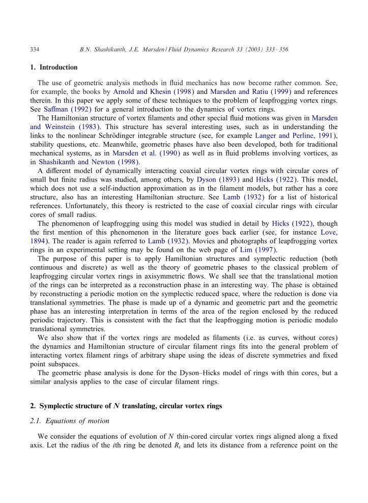
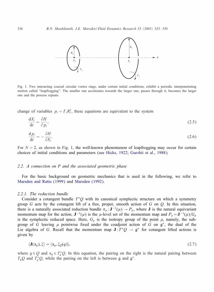
Fig. 1. Two interacting coaxial circular vortex rings, under certain initial conditions, exhibit a periodic interpenetratingmotion called “leapfrogging”. The smaller one accelerates towards the larger one, passes through it, becomes the largerone and the process repeats.

change of variables pi = �iR2i , these equations are equivalent to the system

dXi

dt=

@H@pi

; (2.5)

dpi

dt=− @H

@Xi: (2.6)

For N = 2, as shown in Fig. 1, the well-known phenomenon of leapfrogging may occur for certainchoices of initial conditions and parameters (see Hicks, 1922; Gurzhii et al., 1988).

2.2. A connection on P and the associated geometric phase

For the basic background on geometric mechanics that is used in the following, we refer toMarsden and Ratiu (1999) and Marsden (1992).

2.2.1. The reduction bundleConsider a cotangent bundle T ∗Q with its canonical symplectic structure on which a symmetry

group G acts by the cotangent lift of a free, proper, smooth action of G on Q. In this situation,there is a naturally associated reduction bundle �� : J−1(�) → P�, where J is the natural equivariantmomentum map for the action, J−1(�) is the �-level set of the momentum map and P�=J−1(�)=G�

is the symplectic reduced space. Here, G� is the isotropy group of the point �, namely, the sub-group of G leaving � pointwise 6xed under the coadjoint action of G on g∗, the dual of theLie algebra of G. Recall that the momentum map J :T ∗Q → g∗ for cotangent lifted actions isgiven by

〈J( q); "〉= 〈 q; "Q(q)〉; (2.7)

where q∈Q and q ∈T ∗q Q. In this equation, the pairing on the right is the natural pairing between

TqQ and T ∗q Q, while the pairing on the left is between g and g∗.


2.2.2. A connection on the reduction bundleAs shown in Marsden et al. (1990) (see also Marsden, 1992), when the coadjoint isotropy subgroup

G� is diFeomorphic to S1 or R, there is an interesting connection $ on the reduction bundle �� (seeMarsden et al. (2000) for a generalization of the construction).

Namely, the g� ∼= R-valued connection one-form is given by

$=1

〈�; %〉 �� ⊗ %: (2.8)

We explain the notation. As above, � is a regular value of the momentum map J and P�=J−1(�)=G�.Also, % is a generator of the Lie algebra g� ∼= R, and �� is the canonical one-form on T ∗Q restrictedto J−1(�).

2.2.3. The connection for vortex ringsIn our problem, Q = R2 with coordinates (X1; X2) and G� = G = R. Choose canonical cotangent

coordinates (X1; X2; p1; p2) for T ∗Q. The phase space is P = T ∗Q \ �= (R2 × (R2)∗) \ �. Here weidentify the dual space (R2)∗ with R2 using the standard Euclidean inner product. Accordingly, wemake the identi6cation q = (p1; p2)∈R2.

Now consider the group G = R acting on Q by translations; the group element g∈R acts on(X1; X2) to give (X1 + g; X2 + g). The in6nitesimal generator is given simply by "Q(X1; X2) = ("; "),where "∈ g = R. The momentum map J : (R2 × (R2)∗) \ � → R∗, is easily computed using (2.7)to be

J(X1; X2; p1; p2) = p1 + p2: (2.9)

Thus, the level set J−1(�) is de6ned by the equation p1 + p2 = � and we can use, for example,(X1; X2; p1) as coordinates for this level set. The canonical 1-form on T ∗Q is � = p1 dX1 + p2 dX2.The restriction of � to J−1(�) is thus given by

�� = p1 dX1 + (� − p1) dX2:

Let %∈R, % = 0, be thought of as a generator of the Lie algebra of the translation group. Usingthe general formula (2.8), we 6nd that the Lie algebra-valued connection one-form $ on the bundle�� : J−1(�) → J−1(�)=G := P� is given by

$=p1 dX1 + p2 dX2

p1 + p2=

1�(p1 dX1 + (� − p1) dX2): (2.10)

It should be noted that the above connection is not valid for the zero-momentum case, i.e. whenp1 + p2 = 0. This is interesting in view of the fascinating experiments by Lim and Nickels (1992)on the head-on collision of two circular vortex rings of equal size and equal but opposite strengths.This con6guration corresponds to a zero-momentum case in this canonical model and suggests thatit needs to be extended to handle such cases and to maybe oFer an explanation for the spectacularinstabilities that are triggered by such collisions.


2.2.4. The curvature of $We now compute the curvature of the connection $, a two-form on the space P�. We 6rst recall

the general computation using the exterior derivative and the horizontal lift:

curv($)(u; v) = d$(hor(u); hor(v))

=1

〈�; %〉 d��(hor(u); hor(v))⊗ %

=− 1〈�; %〉 i

∗��(hor(u); hor(v))⊗ %

=− 1〈�; %〉 �

∗��(hor(u); hor(v))⊗ %

=− 1〈�; %〉 ��(u; v)⊗ %;

where �� is the reduced symplectic form on P� and hor(u) and hor(v) are horizontal lifts of vectorsu; v∈T[z]P�, the tangent space of P� at a point [z] = ��(z) and where the horizontal lift is to thepoint z (the answer is of course independent of the choice of representative z of the class [z]).Using its description in terms of the equation p1 + p2 = �, we see that the level set J−1(�) is

diFeomorphic to (R2 ×R) \�. The reduced space P� is diFeomorphic to (R×R) \��, where �� isthe single point that � projects to under ��. The phase portrait on P� is a function of the parametervalues �1, �2, A1 and A2.

In general, for cotangent bundles and reduction by Abelian groups, P�∼= T ∗(Q=G) and the reduced

symplectic form is given, by cotangent bundle reduction theory (see, for example, Marsden, 1992),as

�� = �can + )�; (2.11)

where �can is the canonical symplectic form and )� is a “magnetic term”, a two-form on the reducedspace Q=G�. Since Q=G� is one-dimensional in our problem of two vortex rings, )� = 0.

Choosing coordinates (X1; X2; p1) for J−1(�) and (X1 − X2; p1) for P�, formula (2.11) gives

�� = d(X1 − X2) ∧ dp1:

Alternatively, �� can be calculated directly from the symplectic reduction theorem (Marsden andWeinstein, 1974) as �∗�� = i∗��.

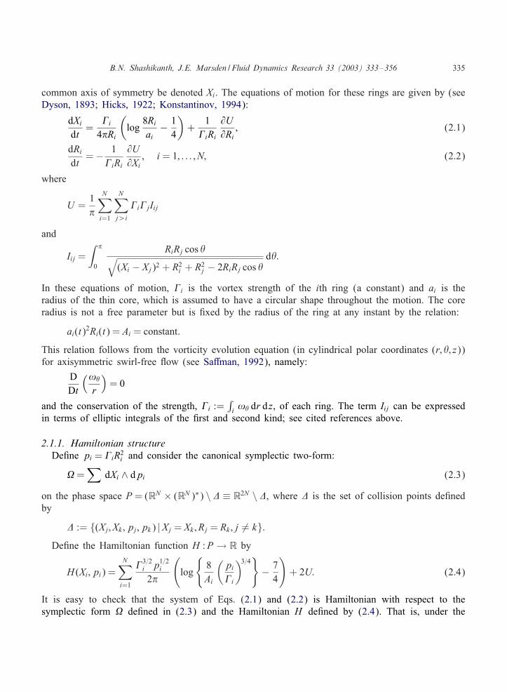
2.2.5. Total phaseThe total phase, Xtot, is that group element which measures the total shift in the symmetry group

direction at the end of one periodic orbit c�(t)∈P�. In general, Xtot =Xd ◦Xg, where Xd is called thedynamic phase, Xg is called the geometric phase and ◦ denotes group composition. In this problem:

Xtot = Xd + Xg:

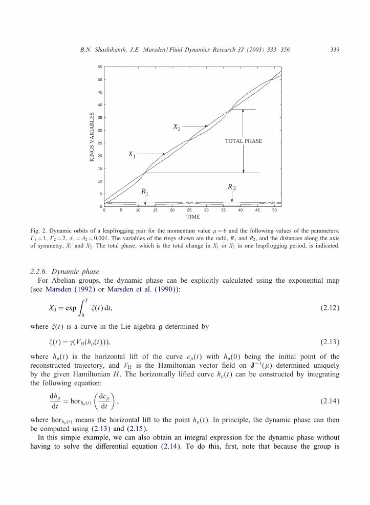
The total phase is indicated for a typical leapfrogging orbit in Fig. 2.


0 5 10 15 20 25 30 35 40 45 500

5

10

15

20

25

30

35

40

45

50

55

TIME

RIN

GS

VA

RIA

BL

ES

TOTAL PHASE

X1

X2

R1R 2

Fig. 2. Dynamic orbits of a leapfrogging pair for the momentum value �= 6 and the following values of the parameters:�1 =1, �2 =2, A1 =A2 =0:001. The variables of the rings shown are the radii, R1 and R2, and the distances along the axisof symmetry, X1 and X2. The total phase, which is the total change in X1 or X2 in one leapfrogging period, is indicated.

2.2.6. Dynamic phaseFor Abelian groups, the dynamic phase can be explicitly calculated using the exponential map

(see Marsden (1992) or Marsden et al. (1990)):

Xd = exp∫ T

0"(t) dt; (2.12)

where "(t) is a curve in the Lie algebra g determined by

"(t) = $(VH(h�(t))); (2.13)

where h�(t) is the horizontal lift of the curve c�(t) with h�(0) being the initial point of thereconstructed trajectory, and VH is the Hamiltonian vector 6eld on J−1(�) determined uniquelyby the given Hamiltonian H . The horizontally lifted curve h�(t) can be constructed by integratingthe following equation:

dh�dt

= horh�(t)

(dc�dt

); (2.14)

where horh�(t) means the horizontal lift to the point h�(t). In principle, the dynamic phase can thenbe computed using (2.13) and (2.15).

In this simple example, we can also obtain an integral expression for the dynamic phase withouthaving to solve the diFerential equation (2.14). To do this, 6rst, note that because the group is


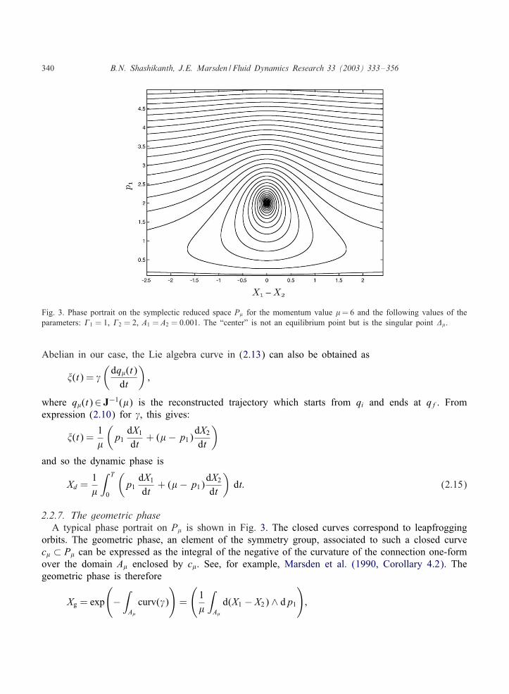
Fig. 3. Phase portrait on the symplectic reduced space P� for the momentum value �=6 and the following values of theparameters: �1 = 1, �2 = 2, A1 = A2 = 0:001. The “center” is not an equilibrium point but is the singular point ��.

Abelian in our case, the Lie algebra curve in (2.13) can also be obtained as

"(t) = $(dq�(t)dt

);

where q�(t)∈ J−1(�) is the reconstructed trajectory which starts from qi and ends at qf. Fromexpression (2.10) for $, this gives:

"(t) =1�

(p1

dX1

dt+ (� − p1)

dX2

dt

)and so the dynamic phase is

Xd =1�

∫ T

0

(p1

dX1

dt+ (� − p1)

dX2

dt

)dt: (2.15)

2.2.7. The geometric phaseA typical phase portrait on P� is shown in Fig. 3. The closed curves correspond to leapfrogging

orbits. The geometric phase, an element of the symmetry group, associated to such a closed curvec� ⊂ P� can be expressed as the integral of the negative of the curvature of the connection one-formover the domain A� enclosed by c�. See, for example, Marsden et al. (1990, Corollary 4.2). Thegeometric phase is therefore

Xg = exp

(−∫A�

curv($)

)=

(1�

∫A�

d(X1 − X2) ∧ dp1

);


where the exponential map exp : g → G in this problem, where G = R under addition, is just theidentity map. Since d(X1−X2)∧dp1 is the standard volume form on P� (also de6ning an orientationon P�), this clearly shows that

Xg =(Area��

);

where Area� is the area enclosed by c�.Finally, we can verify that Xtot =Xd +Xg. For this, rewrite Xg using Green’s theorem in the plane

as

Xg =1�

∫A�

d(X1 − X2) ∧ dp1 =−1�

∮p1 d(X1 − X2) =−1

�

∫ T

0p1

(dX1

dt− dX2

dt

)dt:

One can check that the dynamic trajectories in Fig. 3 are oriented in the counterclockwise sense inthe plane with X1 − X2 and p1 as coordinates, so the parametrization of the curves by time givesthe correct orientation for the use of Green’s theorem. The contour integral in the above is aroundthe closed curve c�(t) in P�. Thus,

Xd + Xg =∫ T

0

dX2

dtdt = Xtot :

2.2.8. A metric description of the connection $As with any connection, $ de6nes a direct sum splitting of the tangent bundle of J−1(�) into

horizontal and vertical vectors. We shall show that this splitting is metrically orthogonal with respectto an interesting metric on J−1(�).

In our case, the horizontal and vertical splitting is given as follows. A vector vq ∈TqJ−1(�) canbe written uniquely as

vq ≡(P

@@p1

; Q@@X1

; R@@X2

)

=(0; K

@@X1

; K@@X2

)+(P

@@p1

; (Q − K)@@X1

; (R− K)@@X2

)

=ver vq + hor vq; (2.16)

where

K =p1Q + (� − p1)R

�: (2.17)

Consistent with this claim, it can be checked that

D��(q)(ver vq) = 0;

($(ver vq))J−1(�) = (0; K; K);

$(hor vq) = 0; (2.18)

where D��(q) is the derivative of the projection map at q.


Consider the following metric on T ∗Q:

〈〈u; v〉〉(X1 ;X2 ;p1 ;p2) = p1u1v1 + p2u2v2 + u3v3 + u4v4:

The restriction of this metric to J−1(�) is

〈〈u; v〉〉(X1 ;X2 ;p1) = p1u1v1 + (� − p1)u2v2 + u3v3:

One checks that the splitting in (2.16) is metric orthogonal. We mention this as a possible link tothe notion of the abstract mechanical connection which is a Lie-algebra valued connection one-formde6ned on the phase space of a system with symmetry. This subject is explored in detail in thepapers of Blaom (2000) and Pekarsky and Marsden (2001).

3. The interaction of N rings of arbitrary shape

In this section we show how the symplectic structure on a coadjoint orbit corresponding to ageneral vorticity distribution in a 4uid domain, which was derived in Marsden and Weinstein (1983),gives a symplectic form and a Hamiltonian vector 6eld on the phase space of N interacting 6lamentrings of arbitrary shapes in R3 (see Fig. 4). We also calculate the momentum map associated withthe SE(3) symmetry of this model and show that this is Ad∗-equivariant. It should be noted that inthis section (and in the next) we choose to model the rings as 6laments, as was done in Marsdenand Weinstein (1983). We believe that the geometric ideas presented here will still have relevanceto more sophisticated ring interaction models which account for core structure.

The Hamiltonian function is still the total kinetic energy of the 4uid but becomes unboundeddue the well-known singularity in the self-induced velocity 6eld (SaFman, 1992). Desingularizationis done by introducing, in the equations of motion, the local induction truncation parameter cj foreach ring. This is a (real) truncation parameter that appears in the local induction approximation(SaFman, 1992; Ting and Klein, 1991) for the self-induced velocity 6eld. It represents a choice ofthe length of the ith ring used to form a 6nite approximation of the unbounded term in the kineticenergy of the 4uid arising due to the singularity.

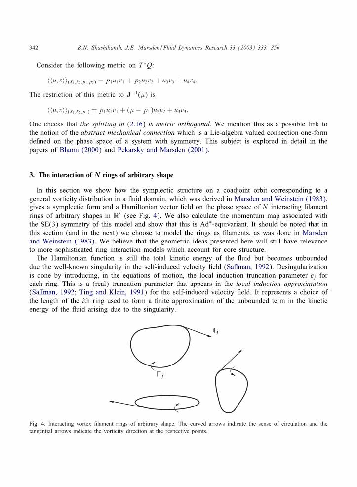
Γ j

t j

Fig. 4. Interacting vortex 6lament rings of arbitrary shape. The curved arrows indicate the sense of circulation and thetangential arrows indicate the vorticity direction at the respective points.


3.1. The energy expression

Consider the kinetic energy of a 4uid of unit density in R3:

H =12

∫〈A(x); !(x)〉 dV;

where the integration is over x∈R3, A :R3 → R3 is the vector potential, ! :R3 → R3 is the vorticity,and the pairing 〈 ; 〉 is the Euclidean inner product on R3. The vector potential satis6es

∇2A =−!

and inverting this standard Poisson equation gives

A(x) =14�

∫!(x′)r′

dV ′;

where r′ =√

(x − x′)2 + (y − y′)2 + (z − z′)2.Let the vorticity be concentrated along N rings of strengths �1; : : : ; �N respectively. As a two-form,

the vorticity is represented, following Marsden and Weinstein (1983), as

!(x; y; z) =∑

�iiti dx ∧ dy ∧ dz 2i(x; y; z); (3.1)

where the operator iti denotes the contraction of the three-form along ti, the unit tangent vector 6eldof the ith ring, and 2i is the delta-function de6ned with respect to arc-length of the ith ring. Thevector potential becomes

A(x) =∑ �i

4�

∮i

ti(s′i) ds′ir′i

;

where r′i =√

(x − x′(s′i))2 + (y − y′(s′i))2 + (z − z′(s′i))2.The kinetic energy can then be written as

H =∑∑

j �=i

�i�j

8�

∮i

∮j

〈tj(s′j); ti(si)〉ds′jr′j

dsi +∑

HiSI; (3.2)

where HiSI is the kinetic energy of self-induction of the ith ring. This term is unbounded and we

desingularize it as follows using the local induction approximation:

HiSI = lim

ci→0

�2

8�

∮i

∫i±ci

〈ti(s′i); ti(si)〉 ds′i√(x(si)− x′(s′i))2 + (y(si)− y′(s′i))2 + (z(si)− z′(s′i))2

dsj;

where i± ci, (ci ¿ 0) indicates that the portion of ring, si− ci ¡ s′i ¡ si+ ci, is ignored in evaluatingthe inner integral. Choosing si and s′i to be arc-length parameters, write

x′(s′i) = x(si) + (s′i − si)dx(si)dsi

+ · · · ;

ti(s′i) = ti(si) + (s′i − si)dti(si)dsi

+ · · ·


and so on. Hence, as ci → 0,

HiSI =

�2

8�

∮i

∫i±ci

ds′i|s′i − si| dsi + O(1)

=�2

8�

∮i

(∫ si−ci

0

ds′i|s′i − si| +

∫ li

si+ci

ds′i|s′i − si|

)dsi + O(1)

=�2

8�

∮i

(−log |s′i − si|si−ci0 + log |s′i − si|lisi+ci) dsi + O(1)

=−�2

4�

∮i

log ci dsj + O(1):

The local induction approximation is the choice of a small non-zero value of ci (or the choice of asmall non-zero lower bound if ci is allowed to vary in time) at each point of the ring and truncatingthe above series to leading order:

HiSI ≈ Hi

LI;

where

HiLI =−�2

4�

∮i

log ci dsi:

In our model we further assume that each ci is 6xed by the initial con6guration of the rings anddoes not vary either with the arc-length si or with time as the rings evolve. This means, in particular,that we do not look at variations in ci while deriving the equations for the interacting rings. Thus,our 6nal expression for the energy is given as follows:

H =∑∑

j �=i

�i�j

8�

∮i

∮j

〈tj(s′j); ti(si)〉ds′jr′j

dsi −∑ �2

i

4�log ci

∮i

dsi: (3.3)

3.2. The symplectic form

For 6xed �1; : : : ; �N the set of all such vorticities forms a coadjoint orbit in the dual of the Liealgebra of volume preserving diFeomorphisms of the 4uid domain. The symplectic structure on thecoadjoint orbit is given by Marsden and Weinstein (1983):

�(Lu!;Lv!) =∫

!(u; v) dV; (3.4)

where u(x; y; z), v(x; y; z) are divergence-free vector 6elds on R3 and the Lie derivatives Lu! andLv! are tangent vectors to the coadjoint orbit at !∈ g∗. Since g∗ is a linear space, the tangentvectors can also be identi6ed with vorticity elements and it can be shown (Marsden and Weinstein,1974) that Lu! ≡ ∇ × (! × u). The vector 6eld ! × u is everywhere normal to ! but is notdivergence-free.


Substituting ! from (3.1) into (3.4) gives

� =∑

�i

∮i

ti · (u(si)× v(si)) dsi =∑

�i

∮i

v(si) · (ti × u(si)) dsi: (3.5)

3.3. The phase space for N vortex loops

The vorticities can be identi6ed with the N curves i.e., with images of N maps (modulore-parametrizations that have the same image) Ci : S1 → R3, Ci(si) = (x(si); y(si); z(si)); i=1; : : : ; N(see Section VI.3 in Arnold and Khesin (1992) for a discussion of this sort of formalism, includingknots). The Hamiltonian is regarded as a functional of these curves.

The phase space P for N 6laments is thus the space of such curves. The tangent space at any pointof the phase space P consists of vector 6elds along the curves. The symplectic form � given by(3.5) can then be viewed as a symplectic form on P. However, � is degenerate and the associatedlinear map from TpP to T ∗

pP has a non-zero kernel consisting of vector 6elds tangential to thecurves at all points. Indeed, since this kernel is a closed subspace Vt ⊂ TpP, one has a direct sumsplitting of the tangent space TpP:

TpP = Vn ⊕ Vt;

v= vn + vt; (3.6)

where v∈TpP, vn ∈Vn, vt ∈Vt , and Vn consists of vector 6elds normal to the curves. The symplecticform �, at each p∈P, therefore acts on the projection of vectors in TpP on to the subspace Vn.

3.4. Computation of functional derivatives

Let 92Ci(si) = (92x(si); 92y(si); 92z(si)) denote (small) variations in the curves. Then,

92ti(si) =(92

dxdsi

; 92dydsi

; 92dzdsi

)=(9d2xdsi

; 9d2ydsi

; 9d2zdsi

):

The functional derivative is de6ned using the pairing between TpP and T ∗pP as follows:⟨

2p;2H2p

⟩=∑∮

i

⟨2Ci;

2H2Ci

⟩dsi :=

∑lim9→0

19(H (Ci + 92Ci)− H (Ci)): (3.7)

We now calculate

lim9→0

19(H (Ci + 92Ci)− H (Ci))

=lim9→0

19

�i

∑j �=i

�j

8�

∮i

∮j

〈tj(s′j); ti(si) + 92ti〉 ds′j√(xi + 92xi − x′j)2 + (yi + 92yi − y′

j)2 + (zi + 92zi − z′j)2dsi

−�2i

4�log ci

∮i

√(d(xi + 92xi)

dsi

)2+(d(yi + 92yi)

dsi

)2+(d(zi + 92zi)

dsi

)2dsi


−�i

∑j �=i

�j

8�

∮i

∮j

〈tj(s′j); ti(si)〉 ds′j√(xi − x′j)2 + (yi − y′

j)2 + (zi − z′j)2dsi

+�2i

4�log ci

∮i

√(dxidsi

)2+(dyi

dsi

)2+(dzidsi

)2dsi

:

Ignoring O(92) and higher order terms we get

lim9→0

19(H (Ci + 92Ci)− H (Ci))

=lim9→0

19

−�i

∑j �=i

�j

8�

∮

i

⟨∮j

〈tj(s′j); ti(si)〉Rij

r3ijds′j; 92Ci

⟩dsi

−∮i

⟨∮j

tj(s′j)rij

ds′j; 92ti(si)

⟩dsi

− �2

i

4�log ci

∮i

〈ti ; 92ti〉 dsi;

where Rij is the position vector of the point (xi; yi; zi) with respect to (x′j; y′j; z

′j) and rij = ‖Rij‖.

Using the elementary identity∮fdgds

ds+∮

gdfds

ds=∮

d(fg) = 0

gives ∮i

⟨2Ci;

2H2Ci

⟩dsi := lim

9→0

19(H (Ci + 92Ci)− H (Ci))

= −�i

∑j �=i

�j

8�

∮

i

⟨∮j


r3ijds′j; 2Ci

⟩dsi

+∮i

⟨ddsi

∮j

tj(s′j)rij

ds′j; 2Ci

⟩dsi

+

�2i

4�log ci

∮i

⟨ddsi

ti; 2Ci

⟩dsi:

Hence,

2H2Ci

=−�i

∑j �=i

�j

8�

∮

j


r3ijds′j +

ddsi

∮j

tj(s′j)rij

ds′j

+

�2i log ci4�

dtidsi

=−�i

∑j �=i

�j

8�

∮

j


r3ijds′j −

∮j

tj(s′j)〈Rij ; ti(si)〉

r3ijds′j

+

�2i log ci4�

dtidsi


=�i

∑j �=i

�j

8�

∮

j

ti(si)×tj(s′j)× Rij

r3ijds′j

− �2

i :i(si) log ci4�

(ti × bi)

=�i

∑j �=i

�j

8�

ti(si)×

∮j

(tj(s′j)× Rij

r3ij

)ni

ds′j

− �2

i :i(si) log ci4�

(ti × bi);

where we have used the Serret–Frenet equations d(ti(si))=dsi=:i(si)ni, :i(si) is the curvature of thering, ni(si) and bi(si) = ti(si)× ni(si) are the unit normal and the unit binormal, respectively, to thering and, in the last line, the subscript ni denotes the component normal to Ci. Note that 2H=2Ci

itself is a vector 6eld normal to Ci.

3.5. Computation of the Hamiltonian vector ,eld

We are now ready to compute the Hamiltonian vector 6eld XH associated to the Hamiltonian Husing the general de6nition �(XH ; u) = dH · u. First of all, write XH = (@C1=@t; : : : ; @CN =@t).Now compute as follows:

�(XH ; vn) = �(XH ; v) = DH (C1; : : : ; CN ) · v

:=∑ ∮

i

⟨vi;

2H2Ci

⟩dsi =

∑ ∮i

⟨(vi)n;

2H2Ci

⟩dsi;

for vn ∈Vn. Hence,∑�i

∮i

vi ·(ti × @Ci

@t

)dsi

=∑

�i

∮i

vi ·ti ×

∑

j �=i

�j

8�

∮j

(tj(s′j)× Rij

r3ij

)ni

ds′j −�i:i(si)log ci

4�bi

dsi

and therefore

@Ci

@t=∑j �=i

�j

8�

∮j

(tj(s′j)× Rij

r3ij

)ni

ds′j −�i:i(si)log ci

4�bi ; i = 1; : : : ; N (3.8)

which are indeed the equations of motion of the rings using the Biot–Savart law and the localinduction approximation.

We summarize this calculation as follows:

Proposition 3.1. The ,lament rings equations of motion (3.8) are Hamiltonian with respect to theHamiltonian function (3.3) and the symplectic structure (3.5).


3.6. The symmetry group

The action of the group G=SE(3)=(SO(3) R3) (the semidirect product of rotations and trans-lations) on the jth 6lament Cj(sj) = (x(sj); y(sj); z(sj)) is simply

g · Cj(sj) = g · (x(sj); y(sj); z(sj)); sj ∈Dom(Cj);

where the right-hand side is the usual SE(3) action on R3. The action on P is then the diagonalaction on the N 6laments. It is straightforward to check that the symplectic form and the Hamiltonianare invariant under this action of SE(3).

The in6nitesimal generator of the G action on P is calculated in a straightforward way:

"P(p) :=d(g(t) · p)

dt

∣∣∣∣t=0

;

where g(t) is the one-parameter subgroup such that g(0) = e and g′(t) = "∈ g ≡ se(3). Note that(Marsden and Ratiu, 1999, Section 14.9) " can be written as the following 4× 4 matrix:

"=

("̂R "T

0 0

);

where "̂R ∈ so(3) is a skew-symmetric 3×3 matrix which can be identi6ed uniquely with an element"R of R3 via the hat map, and "T ∈R3. The one-parameter subgroup can be written as

g(t) = I + t"+ · · ·(Marsden and Ratiu, 1999, p. 251, ex.(b)). Thus, for v∈R3,

g(t) · v= I · v+ t"̂R · v+ t"T + · · ·= I · v+ t"R × v+ t"T + · · ·

Thus for p= [(x(s1); y(s1); z(s1)); : : : ; (x(sN ); y(sN ); z(sN )] = [C1(s1); : : : ; CN (sN )],

"P(p) = ("R × C1(s1) + "T ; : : : ; "R × CN (sN ) + "T ):

Note that "R × Cj(sj) is a vector 6eld normal to Cj but "T is not. Recall that the in6nitesimalgenerator of the group action is the Hamiltonian vector 6eld generated by J ("), a linear real-valuedfunction on the Lie algebra. Thus,∑

�i

∮i

vi · (ti × ("R × Ci(si) + "T )) dsi =∑ ∮

i

⟨vi;

2J (")(p)2Ci

⟩dsi: (3.9)

3.7. The momentum map

We now calculate the momentum map associated with the SE(3) action on P. Recall that (see, forexample, Marsden and Ratiu, 1999) for a Lie group action on a Poisson manifold P, the momentummap J :P → g∗ given by

〈J(p); "〉= J (")(p):

Identifying se(3) with R6, the pairing above is the Euclidean inner product on R6.


From (3.9) we get

�i

∮i

(2Ci; (ti × ("R × Ci(si) + "T ))〉 dsi = lim9→0

19(J (")(Ci + 92Ci)− J (")(Ci)): (3.10)

It can be checked that the following choice of J (") satis6es the above relation:

J (") =

⟨"R;−1

2

∑�i

∮i

(〈Ci; Ci〉ti) dsi⟩

+

⟨"T ;

12

∑�i

∮i

(Ci × ti) dsi

⟩:

To see this, note that

lim9→0

19(J (")(Ci + 92Ci)− J (")(Ci)) =

⟨"R;−�i

∮i

(〈2Ci; Ci〉ti + 1

2〈Ci; Ci〉2ti

)dsi

⟩

+

⟨"T ;

12�i

∮i

(2Ci × ti) dsi +12�i

∮i

(Ci × 2ti) dsi

⟩:

Now use the identities∮i

ddsi

(Ci × 2Ci) dsi = 0 =∮i

(Ci × 2ti) dsi +∮i

(ti × 2Ci) dsi

and ∫i

ddsi

〈Ci〈2Ci; "R〉; Ci〉 dsi = 0 =∮i

2〈Ci; ti〉〈2Ci; "R〉 dsi +∮i

〈Ci; Ci〉〈2ti; "R〉 dsi

to get

lim9→0

19(J (")(Ci + 92Ci)− J (")(Ci))

=− �i

∮i

〈2Ci; ti × (Ci × "R)〉 dsi + �i

∮i

〈2Ci; ti × "T 〉 dsi:

We summarize this calculation as follows.

Proposition 3.2. The momentum map for the SE(3) action on the phase space P of N ,lamentrings is given by

J(p) =

−1

2

∑�i

∮i

(〈Ci(si); Ci(si)〉ti)dsi; 12∑

�i

∮i

(Ci(si)× ti) dsi

: (3.11)

In addition, by Noether’s theorem the components of the momentum map are conserved quantities,usually referred to as the linear and angular impulse of the >uid.


3.8. Equivariance

As is well known, one has to be careful with equivariance of the momentum map in 4uidmechanics. For example, the momentum map associated with the Euclidean group action for thespace of N vortices in the plane is not equivariant if the sum of vortex strengths is not zero(see, for example, Adams and Ratiu, 1988; and Marsden and Ratiu, 1999). However in our case,we have

Proposition 3.3. The momentum map (3.11) is Ad∗-equivariant.

To prove this, note that the coadjoint action of (A; a)∈SE(3) on se(3)∗, after identifying the latterwith R3 × R3, is given as follows (see, for example, Marsden and Ratiu, 1999):

Ad∗(A;a)−1(u; v) = (Au+ a× Av; Av);

where u and v are dual to Lie algebra elements in so(3) and R3, respectively. Writing J(p)= (u; v),we get:

J · ((A; a) · p)− Ad∗(A;a)−1(u; v)

=

−1

2

∑�i

∮i

(〈ACi(si) + a; ACi(si) + a〉Ati) dsi + 12

∑�iA

∮i

(〈Ci(si); Ci(si)〉ti) dsi

−a× 12

∑�iA

∮i

(Ci(si)× ti) dsi;12

∑�i

∮i

((ACi(si) + a)× Ati) dsi

−12

∑�iA

∮i

(Ci(si)× ti) dsi

=

−

∑�i

∮i

(〈a; ACi(si)〉Ati) dsi − a× 12

∑�iA

∮i

(Ci(si)× ti) dsi; 0

=

−1

2

∑�i

∮i

(〈a; ACi(si)〉Ati + 〈a; Ati〉ACi) dsi; 0

=

−1

2

∑�i

∮i

ddsi

(〈a; ACi(si)〉ACi(si)) dsi; 0

=(0; 0):


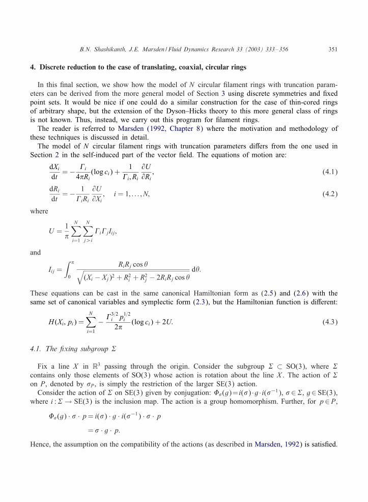
4. Discrete reduction to the case of translating, coaxial, circular rings

In this 6nal section, we show how the model of N circular 6lament rings with truncation param-eters can be derived from the more general model of Section 3 using discrete symmetries and 6xedpoint sets. It would be nice if one could do a similar construction for the case of thin-cored ringsof arbitrary shape, but the extension of the Dyson–Hicks theory to this more general class of ringsis not known. Thus, instead, we carry out this program for 6lament rings.

The reader is referred to Marsden (1992, Chapter 8) where the motivation and methodology ofthese techniques is discussed in detail.

The model of N circular 6lament rings with truncation parameters diFers from the one used inSection 2 in the self-induced part of the vector 6eld. The equations of motion are:

dXi

dt=− �i

4�Ri(log ci) +

1�i; Ri

@U@Ri

; (4.1)

dRi

dt=− 1

�iRi

@U@Xi

; i = 1; : : : ; N; (4.2)

where

U =1�

N∑i=1

N∑j¿i

�i�jIij;

and

Iij =∫ �

0

RiRj cos �√(Xi − Xj)2 + R2

i + R2j − 2RiRj cos �

d�:

These equations can be cast in the same canonical Hamiltonian form as (2.5) and (2.6) with thesame set of canonical variables and symplectic form (2.3), but the Hamiltonian function is diFerent:

H (Xi; pi) =N∑i=1

− �3=2i p1=2

i

2�(log ci) + 2U: (4.3)

4.1. The ,xing subgroup =

Fix a line X in R3 passing through the origin. Consider the subgroup = ⊂ SO(3), where =contains only those elements of SO(3) whose action is rotation about the line X . The action of =on P, denoted by >P, is simply the restriction of the larger SE(3) action.

Consider the action of = on SE(3) given by conjugation: ?>(g)= i(>) ·g · i(>−1), >∈=, g∈SE(3),where i := → SE(3) is the inclusion map. The action is a group homomorphism. Further, for p∈P,

?>(g) · > · p= i(>) · g · i(>−1) · > · p= > · g · p:

Hence, the assumption on the compatibility of the actions (as described in Marsden, 1992) is satis6ed.


In addition, Ad∗-equivariance implies, by restricting to elements of =, that the following is alsotrue:

J · >P = ?∗>−1 ;g · J;

where ?∗>−1 ;g is the dual of ?>−1 ;g, with ?>;g : se(3) → se(3) being the Lie algebra homomorphism

induced by the group homomorphism ?>.

4.2. The ,xed point set

The 6xed point set of the = action on P is

P= = {p∈P|> · p= p for all >∈=}= {N circular 6laments with the common axis X }:

The symplectic form on P= can be obtained from (3.5) by choosing a cylindrical coordinate framewith one axis parallel to the X direction. For normal axisymmetric vector 6elds (xaj ; r

aj ; 0) and

(xbj ; rbj ; 0) we get

�=∑

�j

∮j

〈(0; 0; 1); (0; 0; xaj rbj − xbj raj )〉Rj d�j

=∑

2��j(xaj rbj − xbj r

aj )Rj = �

∑�j d(xj ∧ r2j );

which, apart from a multiplicative factor of �, is the same as (2.3). It should be noted that theHamiltonian for circular 6lament rings derived from (3.2) is � times the Hamiltonian in (2.4) andthe discrete reduction process indeed leads to the same vector 6eld as (2.1) and (2.2). A similarcalculation shows that the only non-zero component of the momentum map (3.11) corresponding tosymmetry along the X -axis, is

J(p) = �∑

�jR2j ;

which again, modulo factor �, is the same as (2.9).

4.3. The ,xed point subgroup

The 6xed point set of the = action on SE(3) is

G= = {g∈SE(3)|?>(g) = g for all >∈=} :However, since = ⊂ SE(3), = ⊂ G=, and hence one seeks only elements of G= \= since only thesehave a non-trivial action on P=. Thus g=(A; a)∈G= if, for all >∈= where > can be written as the3× 3 matrix

> =

1 0 0

0 cos � −sin �

0 sin � cos �

;


in an orthonormal basis (e1; e2; e3) where one of the basis vectors is parallel to the X axis, thefollowing holds:

(A; a) = (>; 0) · (A; a) · (>−1; 0)

= (>; 0) · (A · >−1; a)

= (> · A · >−1; > · a):It is obvious that a = > · a, for all >∈= implies a = X . To 6nd the elements that satisfy the otherequality, assume there exists A ∈ = such that

A · v = > · A · >−1v;

for all >∈= and all v∈R3. Choose a v lying on the X -axis, so that v is invariant with respect tothe = action. Then the above equality implies that A · v = > · A · v which can be satis6ed only ifA∈=. Hence,

G= \ == X

and we can state that:

Proposition 4.1. The system represented by Eqs. (4.1) and (4.2) is a Hamiltonian subsystem ofthe Hamiltonian system represented by Eqs. (3.8) in the following sense: it is obtained by discretereduction with respect to the action of the compact symmetry subgroup = ⊂ SE(3). The phasespace P= of the subsystem is the ,xed point set of the action of = on P. The symmetry group G=

of the subsystem is the ,xed point subgroup G===, where G= is the ,xed point set of the actionof = on SE(3). The Hamiltonian function, symplectic form and momentum map are obtained bysimply restricting to P=.

5. Conclusions and future directions

Two ideas-geometric phases and discrete reduction-from the geometric theory of reduction ofconservative systems with symmetry are applied in this paper to a model of interacting vortexrings in incompressible, inviscid 4uid. The authors view this paper as a preliminary step to moresophisticated modeling of ring interactions using ideas from geometric mechanics. In this respect,considerable progress has already been made in the wider context of the averaged Euler equations.See Holm et al. (1998), Oliver and Shkoller (2000) and Marsden and Shkoller (2003) and referencestherein. The averaged Euler equations may well be the context in which to do more sophisticatedring modeling work since recent results (Holm, 2003) indicate that there is a natural way, consistentwith the fundamental variational principles of mechanics, of desingularizing the self-induced velocity6eld without the introduction of arbitrary parameters as in the local induction approximation. Thesesorts of models are, as discussed in the paper of Holm, related to all the other interesting modelsavailable in the literature; see, for instance Klein and Majda (1993), Klein et al. (1995), Klein andTing (1992) and references therein.

The motivation for modeling ring interactions comes from many diFerent 4uid phenomena ofengineering and physics, many of which involve the presence of rigid or deformable boundaries.


To name a few, the shedding of vortices from the tips of aircraft wings and helicopter blades andthe vortices shed by 6sh (Triantayfyllou and Triantayfyllou, 1995) and birds (Rayner, 1979) duringlocomotion. A long-term goal of our work is to model rings interacting dynamically with movingsolid boundaries. The authors are not aware of any modeling work, even in an inviscid framework(like a vortical extension to KirchhoF’s equations) in this area. Geometric ideas are expected to playkey roles in such an area given the well-known geometry of inviscid vortex models (Marsden andWeinstein, 1983) and that of the system of a solid body interacting dynamically with a potential4ow 6eld (Leonard and Marsden, 1997). Some work in the 2-D case with point vortices instead ofrings has already been done in Shashikanth et al. (2002).

Another future direction suggested by this work and Marsden and Weinstein (1983) is to modelthe dynamical interaction of N interacting vortex rings of general core structure, with no constraintson the mutual separation distances between rings. Apart from extending the ideas in Sections 3and 4 in this paper, such a model could also shed light on the phenomenon of vortex stretchingwhich is still not well understood. It has been conjectured, for example in Constantin and FeFerman(1993), that this phenomenon is linked to the lack of a global existence and uniqueness proof for the3-D Navier–Stokes equations. A related subject on which such a model can have some bearing isthat of the development of 6nite time singularities in solutions of the 3-D Euler and Navier–Stokesequations. For example, in the work by Pelz (1997), it is suggested that a certain con6guration ofvortex rings with thin cores can display such singular behavior. Of course these questions are alsotied up with the issues of the averaged Euler equations since the physical modeling literally by theEuler or Navier–Stokes equations for such singular phenomena is questionable, while working withthe averaged equations, for which there is no such singular phenomena, at least with viscosity, isjust as reasonable (see Foias et al., 2002; Marsden and Shkoller, 2001).Finally, we mention that another interesting future direction is that of variational numerical

schemes, which automatically preserve at the algorithmic level, the basic 4uid dynamical struc-tures, such as vorticity. Of course there are many interesting schemes already available (see, forinstance Knio and Klein, 2000), but variational schemes are interesting for long time simulations, asthe work of Rowley and Marsden (2002) on planar point vortices shows and it would be interestingto extend this to the case of vortex rings.

Acknowledgements

The authors would like to thank Darryl Holm and Paul Newton for useful discussions and sugges-tions. BNS would also like to thank Sergey Pekarsky for some preliminary discussions on cotangentbundle connections.

References

Adams, M.R., Ratiu, T.S., 1988. The three point vortex problem: commutative and noncommutative integrability. In:Meyer, K. Saari, D. (Eds.), Hamiltonian Dynamical Systems, Contemp. Math. 81, 245–257.

Arnold, V.I., Khesin, B., 1992. Topological methods in hydrodynamics. Ann. Rev. Fluid Mech. 24, 145–166.Arnold, V.I., Khesin, B., 1998. Topological Methods in Hydrodynamics, Applied Mathematical Sciences 125, Springer,

Berlin.


Blaom, A.D., 2000. Reconstruction phases via Poisson reduction. DiFerential Geom. Appl. 12 (3), 231–252.Constantin, P., FeFerman, C., 1993. Direction of vorticity and the problem of global regularity of the Navier–Stokes

equations. Indiana Univ. Math. J. 42 (3), 775–789.Dyson, F., 1893. The potential of an anchor ring—Pt. II. Philos. Trans. Roy. Soc. London Ser. A 184, 1041–1106.Foias, C., Holm, D.D., Titi, E.S., 2002. The three dimensional viscous Camassa–Holm equations and their relation to the

Navier–Stokes equations and turbulence theory. Dyn. DiFerential Equations 14, 1–36.Gurzhii, A.A., Konstantinov, M.-Yu., Meleshko, V.V., 1988. Interaction of coaxial vortex rings in an ideal 4uid. Fluid

Dynam. 23, 224–229. Consultants Bureau, New York (translated from Izv. Akad. Nauk SSSR Mekh. Zhidk. Gaza1988, OVYR, 2, 78–84 (in Russian)).

Hicks, W.M., 1922. On the mutual threading of vortex rings. Proc. Roy. Soc. London Ser. A 102, 111–131.Holm, D., 2003. Rasetti–Regge Dirac bracket formulation of Lagrangian 4uid dynamics on vortex 6laments. Math. Comput.

Simulation 62, 53–63.Holm, D.D., Marsden, J.E., Ratiu, T.S., 1998. The Euler–PoincarUe equations and semidirect products with applications to

continuum theories. Adv. Math. 137, 1–8.Klein, R., Majda, A.J., 1993. An asymptotic theory for the nonlinear instability of antiparallel pairs of vortex 6laments.

Phys. Fluids A 5, 369–379.Klein, R., Ting, L., 1992. Vortex 6lament with axial core structure variation. Appl. Math. Lett. 5, 99–103.Klein, R., Majda, A.J., Damodaran, K., 1995. Simpli6ed equations for the interaction of nearly parallel vortex 6laments.

J. Fluid Mech. 288, 201–248.Knio, O.M., Klein, R., 2000. Improved thin-tube models for slender vortex simulations. J. Comput. Phys. 163, 68–82.Konstantinov, M.Yu., 1994. Chaotic phenomena in the interaction of vortex rings. Phys. Fluids 6, 1752–1767.Lamb, H., 1932. Hydrodynamics, 6th Edition. Dover, New York.Langer, J., Perline, R., 1991. Poisson geometry of the 6lament equation. J. Nonlinear Sci. 1, 71–94.Leonard, N.E., Marsden, J.E., 1997. Stability and drift of underwater vehicle dynamics: mechanical systems with rigid

motion symmetry. Physica D 105, 130–162.Lim, T.T., 1997. http://www.eng.nus.edu.sg/mpelimtt/TT LIM.htm.Lim, T.T., Nickels, T.B., 1992. Instability and reconnection in the head-on collision of two vortex rings. Nature 357,

225–227.Love, A.E.H., 1894. On the motion of paired vortices with a common axis. Proc. London Math. Soc. 25, 185–194.Marsden, J.E., 1992. Lectures on Mechanics, London Mathematical Society Lecture Note Series, Vol. 174. Cambridge

University Press, Cambridge.Marsden, J.E., Montgomery, R., Ratiu, T.S., 1990. Reduction, Symmetry and Phases in Mechanics, Memoirs, Vol. 436.

American Mathematical Society, Providence, RI.Marsden, J.E., Ratiu, T.S., 1999. Introduction to Mechanics and Symmetry, Texts in Applied Mathematics, 2nd Edition.

Vol. 17, Springer, Berlin, 1999.Marsden, J.E., Ratiu, T.S., Scheurle, J., 2000. Reduction theory and the Lagrange–Routh equations. J. Math. Phys. 41,

3379–3429.Marsden, J.E., Shkoller, S., 2001. Global well-posedness of the LANS- equations. Proc. Roy. Soc. London 359,

1449–1468.Marsden, J.E., Shkoller, S., 2003. The anisotropic averaged Euler and Navier–Stokes equations. Arch. Rat. Mech. An.

166, 27–46.Marsden, J.E., Weinstein, A., 1974. Reduction of symplectic manifolds with symmetry. Rep. Math. Phys. 5, 121–130.Marsden, J.E., Weinstein, A., 1983. Coadjoint orbits, vortices and Clebsch variables for incompressible 4uids. Physica D

7, 305–323.Oliver, M., Shkoller, S., 2000. The vortex blob method as a second-grade non-Newtonian 4uid; E-print,

http://xyz.lanl.gov/abs/math.AP/9910088/.Pekarsky, S., Marsden, J.E., 2001. Abstract mechanical connection and abelian reconstruction for almost KGahler manifolds.

J. Appl. Math. 1, 1–28.Pelz, R., 1997. Locally self-similar 6nite time collapse in a high-symmetry vortex 6lament model. Phys. Rev. E 55,

1617–1626.Rayner, J.M.V., 1979. A vortex theory of animal 4ight. Part 2. J. Fluid Mech. 91, 731–763.Rowley, C.W., Marsden, J.E., 2002. Variational integrators for point vortices. Proc. CDC 40, 1521–1527.

http://www.eng.nus.edu.sg/mpelimtt/TT_LIM.htm

http://xyz.lanl.gov/abs/math.AP/9910088/


SaFman, P.G., 1992. Vortex Dynamics. Cambridge Monographs on Mechanics and Applied Mathematics. CambridgeUniversity Press, Cambridge.

Shashikanth, B.N., Marsden, J.E., Burdick, J.W., Kelly, S.D., 2002. The Hamiltonian structure of a 2-D rigid circularcylinder interacting dynamically with N point vortices. Phys. Fluids 14 (3), 1214–1227.

Shashikanth, B.N., Newton, P., 1998. Vortex motion and the geometric phase. Part I. Basic con6gurations and asymptotics.J. Nonlinear Sci. 8, 183–214.

Ting, L., Klein, R., 1991. Viscous Vortical Flows Lecture Notes in Physics, Vol. 374. Springer, Berlin.Triantayfyllou, M.S., Triantayfyllou, G.S., 1995. An eVcient swimming machine. Sci. Am. 272, 64–70.

Documents

Leapfrogging vortexrings: Hamiltonian structure, geometric