Embed Size (px)
Citation preview

Leading the Herd to Greener Pastures: When Trade Imitation is the Most “Profitable” Form of Flattery Kingsley Fong, David R. Gallagher, Peter Gardner, and Peter L. Swan∗
School of Banking and Finance, The University of New South Wales
Abstract
We find that relatively large institutional trade packages that are spread across multiple brokers and
multiple days contain information about market fundamentals. We show that fund managers
executing these packages are leaders, in the sense that other managers subsequently follow with
packages on the same side in the same securities. This following behavior, or herding, is rational to
the extent that early followers profit from their trades. Although some leaders subsequently reverse
their positions, the price effects associated with these initial trades are not reversed, establishing that
leaders’ and followers’ trades enhance price discovery.
Copyright © 2006 Kingsley Fong, David R. Gallagher, Peter Gardner, and Peter L. Swan. All rights reserved.
∗Fong, [email protected], (+612) 93854932, Gallagher, [email protected], (+612) 92369106, Gardner, [email protected], (+612) 92369153, Swan, [email protected], (+612) 93855871, School of Banking and Finance, The University of New South Wales, Sydney, N.S.W. 2052 Australia. The authors thank an anonymous referee, the editor (Hendrik Bessembinder), as well as David Feldman, Marty Gruber, Stefan Ruenzi, Richard Sias, and Terry Walter, for helpful comments. The authors also express their thanks to Portfolio Analytics and the Securities Industry Research Center of Asia-Pacific (SIRCA) for the provision of data. The authors gratefully acknowledge research funding from the Australian Research Council (DP0346064), and Peter Gardner acknowledges receipt of a Financial Integrity Research Network (FIRN) scholarship as the best doctoral consortium paper prize. We also thank the organizers of the 2006 EFMA Conference in Madrid for the award of the best conference paper prize. An earlier draft of this paper was entitled “A Closer Examination of Investment Manager Herding Behavior.”

2
I. Introduction
We examine how information becomes reflected in stock prices as a consequence of the trading
decisions of competing fund managers who actively pick stocks. This process of price discovery has
previously been approached from two different directions. One is mimicking behavior, in which one
investor copies the trades of another by trading in the same stock and in the same direction; this is
known as herding (see, for example, Wermers (1999)). While many definitions of herding have
been proposed, it is likely to be captured best by “correlated trading across institutional investors”
(Lakonishok, Shleifer and Vishny (1992) p. 25—hereafter LSV).1
The second approach to price discovery is the choice of an optimal trade size by informed
investors wishing to camouflage their desired orders by spreading them over time (Kyle (1985)).
Barclay and Warner (1993) show that informed investors split large packages of orders up into
medium sized trades. These information-rich medium-sized trades are largely initiated by
institutional investors (Chakravarky (2001)). We merge these two approaches by first identifying
information events in the form of disguised trade packages and then investigate the responses of
would-be followers to these events.
We combine the trades of active fund managers into trade packages (hereafter, packages) using
the approach of Chan and Lakonishok (1995) to reveal more clearly the stealth-like nature of
strategic trading. Two characteristics of these packages are investigated: (i) the number of days over
which each package is spread, and (ii) the number of brokers used to execute each package. We
hypothesize that both of these elements contribute to disguise the size of the package. Further, such
disguise is designed to reduce market impact during the execution by not revealing to brokers and
fellow traders the true package size. This incentive to disguise is larger for informed packages than
for liquidity-motivated packages, the latter having no permanent price impact.
We show that better disguise through the use of two or more brokers leads to (i) higher returns
over the subsequent year, and (ii), seemingly in contradiction to the hypothesis that disguise aims to
minimize market impact, greater price impact over the duration of the package than for equivalent

3
single-broker packages. We conclude from this surprising finding that there is a positive association
between the degree of disguise and the extent to which a package is information-motivated.
Consequently, we define these packages utilizing multiple brokers as information events and
call them leader packages. We assess the extent of fund managers following leader packages by
counting the number of fund managers who subsequently trade on the same side in the same
security. This procedure identifies what we call the number of followers; recognizing that some of
these packages might be coincidental or might represent a delayed response by other managers to
the same information received by the leader.
We then empirically examine the profitability of the sequence of follower packages. We use
two-stage least squares (2SLS) to show how the profitability of being a leader is affected by the
number of followers. We use 2SLS because we recognize that the number of followers is not
exogenous but depends on the level of disguise adopted by the leader. In the first stage we forecast
the number of followers for all manager packages, whether disguised via multiple brokers or not.
We find that disguise involving the use of multiple package days is related negatively to the number
of followers. Disguise is effective; despite our surprising finding, referred to above, of a positive
association between the use of disguise and package price impact.
In the second stage we explain the one-year excess returns of the leader packages in terms of the
number of package-days, i.e., the number of days over which the package is spread, and the number
of brokers employed, as well as the predicted number of followers from the first stage. We find that
leader profitability diminishes in the number of followers and increases in the two measures of
disguise, namely package days and number of brokers employed. We conclude that fund managers
act rationally by attempting to disguise the nature of leader packages through the use of multiple
brokers.
We find that following the leader is profitable up to the seventh follower. From this we
conclude that it is rational for managers to follow. However, this apparent following might
represent slower reactions to the same informational signal received by the leader, and thus might

4
not be deliberate. There are two reasons for believing that following is deliberate. First, the
disguising actions of the leader indicate that its purpose is to make following more difficult, and
thus suggest that following is deliberate, even though there may be other reasons for disguise.
Second, a manager is more likely to follow the package of a high-reputation leader with previous
trading success. While both reasons are strongly suggestive that following is deliberate, they may
not be conclusive. For example, high-reputation managers might be systematically quicker to act on
information.
Strikingly, these leader-follower packages continue to be profitable for the subsequent twelve
months. In other words, there is no evidence of price reversal. Moreover, this indicates that leaders
do reluctantly take their herd to greener pastures. This is despite the fact that they devote their best
efforts to avoid becoming leaders. We conclude that following by the first six managers speeds the
price discovery process. This long-term profitability is consistent with the thesis that herding
enhances price discovery. By contrast, in the market microstructure literature (for example, Keim
and Madhavan (1996)) it is common for price reversal to be measured after as little as a few
seconds, minutes, or one or more subsequent trades.
The excess returns from following imply that leader managers fail to completely exploit their
superior information. We find evidence suggesting that this is a result of portfolio risk constraints,
where the manager limits the portfolio’s relative weight in stocks with respect to the market index.
We also find that while it is common for leaders to reverse their positions in the next year, they
do not appear to be deliberately manipulating followers. An exploitative strategy might involve
promoting (or ramping) a stock by falsely announcing an informed trade to a would-be mimicker
and then selling out to the follower at the artificially created bubble peak. In fact, leaders could have
done better still by further delaying trade reversal, suggesting a risk reduction motivation.
Moreover, only a small minority of leader purchases are subsequently sold to followers. Overall, we
observe that herding behavior is beneficial to the market as a whole. From a public policy

5
perspective, fund manager herding appears to be information-based and non-manipulative,
motivationally speaking.
A number of empirical studies have focused on the existence of institutional herding activity
and its impact on stock prices (for example, see LSV, Grinblatt, Titman, and Wermers (1995),
Wermers (1999), Nofsinger and Sias (1999), Sias (2004), Wylie (2005), and Kim and Nofsinger
(2005)). This literature provides evidence of herding in the U.S., U.K., and Japanese markets as
associations or commonalities in trading behavior. For example, how many fund managers are
likely to be trading in the same stocks and in the same direction over the same time period? LSV (p.
24) and subsequent researchers find that, while there tends to be more herding in smaller stocks,
even here the magnitude is not dramatic. This traditional approach may not tell us a great deal about
the motives of the participants. However, some of these studies, such as Wermers (1999) do tell us
that such correlated trading is beneficial to market efficiency, as it is strongly associated with price
discovery. Thus, this tradition is complementary to our own information-event focused approach
In contrast to our findings and those of Wermers (1999), the theoretical herding literature has
suggested that herding is harmful to market efficiency. This is because it involves fund managers’
ignoring their own private information in favor of mimicking another manager’s trades. For
example, poor performance appears to be more tolerated so long as all herding managers are in the
same unenviable position (see Scharfstein and Stein (1990) and Froot, Scharfstein, and Stein
(1992)). Likewise, managers may infer that competing fund managers hold private information (due
to their prior trades), resulting in the formation of informational cascades (Banerjee (1992),
Bikhchandani, Hirshleifer, and Welch (1992), and Avery and Zemsky (1998)). Informational
cascades are like fashions and fads, and occur when it is optimal for a manager to follow an earlier
trade and to ignore his own private information. Thus the high-tech bubble that burst in 2000 may
have been a fad due to fund manager herding based on uninformed leader packages. 2 We find no
evidence to suggest that followers ignore their own potentially superior private information.
6
Much of this literature leaves open the mechanism by which fund managers observe the
disguised leader packages. Word of mouth transmittal is the focus of Hong, Kubik, and Stein
(2005). Another mechanism is inference from the identities of brokers. Over the period of our study,
broker identities were transparent, but only to other fellow brokers, on every order prior to the trade.
Under the rules at least, this information could not be passed on to clients, although there were
many allegations that these rules were breached (see Bartholomeusz (2003)).
The remainder of this paper is organized as follows. Section II describes the data. For
comparison with the literature, Section III contains the research design and empirical results, based
on the herding measure used in previous studies over monthly and quarterly intervals. For
robustness, we also employ the herding measure proposed by Sias (2004).3 In Section IV, we
present the trade package approach to study leader and follower relationships. Our conclusions are
presented in the final section.
II. Data
A. Description of Databases
Our sample comprises 30 active equity managers, sourced from the Portfolio Analytics
Database. Individual fund managers provided daily trade summaries and monthly holdings,
together with broker identification for each trade, under conditions of strict confidentiality. The
sample period of this study is 2nd January 1994 to 31st December 2001.
The information in the database we constructed was elicited by invitation from active
investment managers operating in Australia, based on total funds under management.4 We asked the
investment managers to provide portfolio information for their two largest active institutional
Australian equities funds.5 For this study, thirty-eight funds comprise the total sample, with the
portfolios benchmarked against either the S&P/ASX 200 or S&P/ASX 300 accumulation indices.6
This database comprises a sample that is representative of the Australian investment management
industry, and includes six of the ten largest managers, six from the next ten, and four from those

7
managers ranked 21-30 (measured by funds under management as of 31 December 2001). The
sample also includes six boutique firms that manage less than AUD$100 million each.
Due to this data collection procedure, we need to assess data issues such as survivorship and
selection bias. Funds have been included in the database only where they have continued to survive
until the collection date. Consequently, only data from “successful funds” are included, hence
potentially overstating performance. Similarly, selection bias may also be present, in that it is
possible that managers who contributed data were more successful than non-contributors.
Studies including Grinblatt, Titman, and Wermers (1995) show that funds that engage in
herding tend to earn higher returns; thus, these biases may also overstate the level of herding.
However, we have the opportunity to gain insight into these possible effects by comparing the fund
returns of managers in our study with the returns for the population of investment managers
(including non-surviving funds) sourced from the Mercer Investment Consulting Manager
Performance Analytics (MPA) database. Over the period of our study, the average manager across
the entire industry outperformed the S&P/ASX 300 by 1.78 percent per annum, with a standard
deviation of 1.39 percent. The mean manager in our sample group outperformed the industry
average by 0.35 percent per annum.7 The level of out-performance for our sample is small
compared with the performance dispersion of the industry; therefore we can conclude that
survivorship and selection bias are unlikely to be significant problems for our study.8
A number of funds in the sample invest in derivative securities. We calculate the effective
exposures of options using the method outlined by Pinnuck (2003), where we calculate the delta of
the option following the Black-Scholes option-pricing model. We then add the effective exposures
to the stock holdings value. We ignore index options and futures, as they do not affect the
preference of the fund manager for particular stocks. It is also important to note that our adjustment
for option securities overcomes one of the limitations of previous U.S. studies, given that the
Security and Exchange Commission’s (SEC’s) 13F filings require, at best, only quarterly stock
holdings data to be disclosed without any requirements for derivative securities.9
8
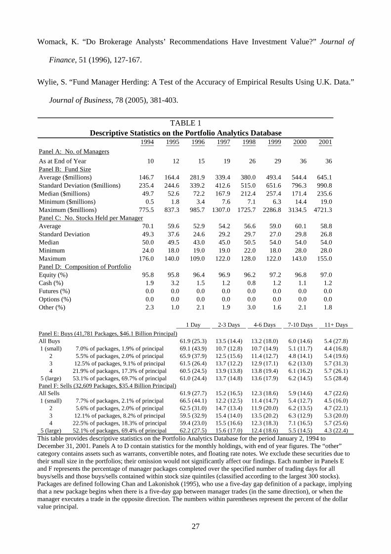
We present descriptive statistics on the Portfolio Analytics Database in Table 1. Panel A shows
that the number of funds across years varies from ten to thirty-six. Panel B illustrates the high
variability in fund sizes, with a large number of small funds, but a concentration of investor assets
among the few largest funds. Panel C shows that the average number of stocks held by each fund is
approximately sixty. Panel D reveals that the active equity managers hold over 95 percent of
portfolio assets in equities.
(INSERT TABLE 1)
We supplement our database with stock price data sourced from the ASX Stock Exchange
Automated Trading System (SEATS) in order to ensure pricing consistency. SEATS contains all
trade information for stocks listed on the ASX, stock-specific data such as market capitalization,
and public earnings announcements contained in the ASX Signal G Database. Index changes to the
S&P/ASX 300 Index are also located in the SEATS Database. We collect these data via a direct
feed from the electronic trading systems of the ASX. (These data have been used previously in
Aitken, Frino, McCorry, and Swan (1998), and Jackson (2005), and even earlier ASX data by
Aitken, Garvey, and Swan (1995)).
B. The Australian Equity Market
The Australian market is both small and developed, and provides a unique environment for
examining herding activity. This is due primarily to the concentrated nature of both (a) stocks listed
on the ASX and (b) investment manager funds under management. According to ASSIRT (2002),
the largest ten investment managers hold 58 percent of total assets under management (AUD$399.9
billion out of AUD$688.9 billion). There is a pronounced level of concentration in Australian equity
investments. The ten largest investment managers control 69 percent of the total Australian equity
9
assets. There is also a high level of concentration amongst stocks in the S&P/ASX 300. The ten
largest stocks account for 48 percent of the index, the fifty largest, 82 percent.
This higher level of concentration in the Australian market may lead to a reduced level of
herding. Active investment managers are required to hold a higher proportion of total funds in
similar stocks. Institutional investors also trade more frequently than the average investor does.
Thus, in a concentrated market, managers are more likely to trade with fellow investment managers,
reducing the level of herding that is possible (see the next section for LSV herding measure).
Intuitively, if the funds in our sample were to make up 100 percent of the market, then no herding
could be possible, as for each buyer there must also be a seller. Broker activity in Australia is also
concentrated among the largest firms, leading to a convergence in information flow, as the trades of
competing managers may be revealed (whether intentionally or not) by the brokers employed.
III. LSV Contemporaneous Herding Measure
In the introduction we mentioned that the empirical herding literature utilizes the
LSV herding measure. To establish that the change in the monthly and quarterly snapshots
of our daily data provide very similar estimates of contemporaneous herding, and are thus
similar to U.S. fund manager data, we now replicate these studies using our dataset.
A. The LSV Herding Measure
LSV defines the Herding Measure, H ti, , for stock i and period t as follows:
(1) |]][[||][| ,,,,, tititititi pEpEpEpH −−−= ,
where pi,t is the proportion of managers who had a net purchase in stock i during period t. We
calculate Hi,t only for periods when five or more managers are trading in the same stock. For
robustness, we calculate Hi,t using alternative minimum numbers of managers, yielding similar

10
results. E[pi,t] is proxied by pt, the proportion of all trades that are buys during period t, thereby
staying constant across stocks and changing only over time. Subtracting E[pi,t] from pi,t controls for
market-wide net fund flows driving purchase decisions. The second adjustment factor E[|pi,t - pt |] is
subtracted to account for random variation around the expected proportion of buyers under the
assumption of independent trading decisions by investment managers. We employ a binomial
distribution to calculate this factor. This herding measure computes the proportion of managers
trading on one side of the market, above the random proportion. Values of Hi,t that are significantly
different from zero indicate herding behavior.
We divide this herding measure into buy-side herding (BHit) and sell-side herding (SHit), (i.e.,
when more managers are buying (selling) than the average proportion of managers), expressed as:
(2) , , , ,| [ ], i t i t i t i tBH H p E p= > and
(3) ][| ,,,, titititi pEpHSH <= .
In order to measure the effect of various stock characteristics, the securities are partitioned into
quintiles for size (market capitalization), book-to-market ratio, earnings yield (earnings per share
divided by stock price), and momentum (prior six month return, following Jegadeesh and Titman
(2001)). We calculate quintiles for book-to-market, earnings yield and momentum, based on the
largest 300 stocks, which account for over 90 percent of the total market capitalization on ASX due
to the concentration of trades executed in the largest stocks. Limiting quintiles ranking to the largest
300 stocks prevents smaller and less liquid stocks from causing bias to the composition of the
quintiles. The size groups also balance the trading activities engaged by the managers, where the
largest 30 stocks comprise the first group; stocks 31-70, the second group; 71-120, the third; 121-
200, the fourth; and stocks greater than 200 the fifth.10
B. Empirical Results
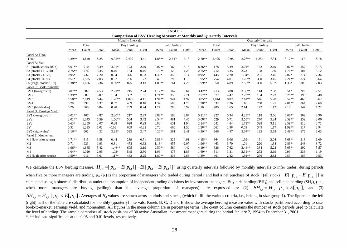
In Table 2 we present the levels of herding using the LSV measure. The overall level of herding
calculated using monthly (or quarterly) holdings in Panel A is 1.39 (or 2.70) percent. This estimate

11
indicates that if one hundred funds are trading in a particular stock, then approximately one (or
three) more fund(s) would be trading on the same side of the market than would be expected if all
managers traded in a random and independent manner. This result is comparable with previous U.S.
(Wermers (1999)), U.K. (Wylie (2005)), and Japanese studies (Kim and Nofsinger (2005)),
indicating a similarity between Australian and foreign markets. The increased herding level from
monthly to quarterly intervals could be an artifact of lengthening the measurement horizon. First,
aggregating trades over longer periods lowers the risk of classifying follower packages into separate
periods, and hence it increases this contemporaneous herding measure. Second, a longer
measurement horizon also increases the risk that we may aggregate independent trades as if they are
herding trades.11 This measurement horizon issue illustrates an important weakness in
contemporaneous herding measures.
We find managers display greater levels of herding when selling. This is consistent with the
findings of Wermers (1999), but is in contrast to the findings of Grinblatt, Titman, and Wermers
(1995) who find greater levels of herding on the buy-side. This suggests that active managers are
more likely to sell than buy in herds. Consistent with Wermers (1999), in Panels B-D of Table 2 we
also find that herding is greatest in small growth stocks, as the precision of information concerning
these stocks is likely to be lower. Panel E shows that momentum trading appears unrelated to
herding in the Australian market.
(INSERT TABLE 2)
IV. Informed Packages Approach to Herding
This study uses a leader-follower packages framework to study herding. We first define trade
packages and identify packages that are likely to be informed. Second, we assess the extent to
which other fund managers follow these informed packages. Third, we examine the profitability of

12
leader and follower packages. Then we attempt to identify the characteristics of lead managers.
Finally we study leader risk constraints and post-package returns.
A. Defining Packages
We adopt the package definition of Chan and Lakonishok (1995), who show that managers
trade stocks over multiple days to minimize trading costs and market impact. They use a five-day
gap definition of a package, implying that a new package begins when there is a five-day gap
between manager trades (in the same direction), or when the manager executes a trade in the
opposite direction. Table 1 reports the frequency distribution of packages for both package length
and stock size quintiles.12 Panels E and F contain the statistics for buys and sells, respectively.
These results show the benefit of using a package methodology, as institutions complete only 25.3
(27.7) percent of buy (sell) volume in one day. Note also that the thirty largest stocks account for
52.1 to 53.1 percent of the number of all packages. We find that the mean institutional package is
84 percent of the average daily trading volume and is thus very large. Even for large firms,
packages average 64 percent of the average daily trading volume. From these statistics, we see the
need for managers to break up trades over multiple days in order to minimize the price impact of
trading. A crucial part of this process of minimizing impact is to make the package less visible to
would-be followers. The distribution of packages is broadly consistent with Chan and Lakonishok
(1995) who report that 20.1 (22.1) percent of total buy (sell) package volume is completed in one
day and note a mean package size of 0.66 relative to normal trading volume.
B. Identifying Informed Packages
In the second step, we identify those manager packages that are likely to contain information.
Chiyachantana, Jain, Jiang, and Wood (2004) suggest that managers who wish to lower market
impact costs will complete packages over multiple days using multiple brokers, but the same tactic
will lessen the chance of being followed. Fund manager trades are signals to the broker executing

13
the trade, and more generally to the market, of fund managers’ views concerning the prospects of
that stock (following Kyle (1985)). As trade size increases, the likelihood that that trade is informed
also increases. Therefore, fund managers reveal less information to brokers and fellow investment
managers by splitting their orders across multiple brokers. However, we do not claim that using this
multiple-broker criterion identifies all informed packages, which is neither necessary nor possible in
our study.
Our data suggest that 26 (or 28) percent of buy (or sell) package volume is completed using
multiple brokers. Not surprisingly, managers complete these larger packages over longer periods.
We also find that these informed packages are associated with significantly fewer packages in the
preceding five days than an average package, providing further support for our hypothesis that these
packages tend to lead the actions of fellow managers.
Table 3 provides evidence that multiple broker packages are informed. Buy packages involving
multiple brokers have a greater return over the execution period of the package, as well as a greater
250-day return from the start of the package, than do similar sized purchases completed using one
broker over one day (see Start to VWAP (volume-weighted average price) in column three).
(INSERT TABLE 3)
When we match similar-sized buy packages completed over the same number of days for trades
using either one broker or two or more brokers, we find that the execution period return is
significantly higher for purchases using two or more brokers (see column six). This suggests that
using one broker has a lower stock price impact. Alternatively, this indicates that managers are not
only using multiple brokers to minimize market impact (which indeed raises the question of why
managers wouldn’t use this tactic for all their trades), but are also using multiple brokers to execute
their most profitable trades. These packages, which are motivated by valuable information, would
presumably have an even greater impact on price had they been executed using a single broker.
Other brokers/managers might witness multiple large trades using the same broker and assume that

14
an informed trader is in the market, or that the broker himself might reveal non-specific information
regarding the trades of the fund manager to other clients trying to generate higher brokerage.
Supporting this second proposition is the statistically significant positive excess return difference
between the one-year return earned by multiple broker and single broker packages (see the bottom
two rows in Table 3, Start to End + 1year).
Moreover, it is intuitive for brokers, who provide valuable information to investment managers,
to be rewarded by the recipient manager trading exclusively with the information-providing broker.
Hence the use of multiple-broker packages suggests that the investment manager may have acquired
information independently of brokers that is exclusive to that investment manager.
For robustness, we examine three variations on the analysis to date. First, we use two alternative
definitions of informed packages: (i) where managers complete large packages over a short time
period; and (ii) where managers increase (decrease) their portfolio weight from zero (above index)
weight to above index (zero) weight for buys (sells). Second, we calculate excess return using the
method developed by Daniel, Grinblatt, Titman, and Wermers (1997) (hereafter DGTW return),
modified by Gallagher and Looi (2006) for the Australian context. Third, we match trades by a
variety of methods: by trade size, by number of package days, and by trades of the same manager in
the same stock, either of the same size or in the same year. All these additional tests yield consistent
findings.
Unreported pre-trade return data suggest managers employ multiple brokers after periods of
high return in order to minimize market impact, and possibly also the number of followers, by
attempting to disguise the identity of the investment manager placing the trades. This suggests that
our result might be due to the momentum effect, where managers commonly purchase stocks with
the highest prior-six-months return, which outperform over the next year (documented in Australia
by Demir, Muthuswamy and Walter (2004)). To examine this possibility further, we first calculate
the DGTW return, which accounts for the momentum factor, yielding similar results. These findings
reveal that the stocks purchased by fund managers earn higher returns than other stocks having

15
similar momentum, and suggest that managers have stock-specific information in addition to
exploiting momentum strategies. Second, we divide our trades into quintiles based on the prior-six-
months return. We then compare the fund manager’s return to S&P/ASX 300 stocks in the same
momentum quintile. Manager trades outperformed the index over the next ninety days in four of the
five quintiles, underperforming only in quintile 4. This further supports our hypothesis that multiple
broker trades contain valuable information, rather than being wholly based on momentum
strategies.13
In another test (unreported), we find that the results for sell packages are consistent. Both
purchase and sale results lead us to conclude that packages using two or more brokers contain more
information than similar packages using one broker. However, as our database includes long-only
funds, managers can generate excess returns from purchases, but are constrained by a zero-weight
position for sales. Hence, throughout the remainder of our analysis we concentrate only on buy
packages.
C. Leader-Follower Behavior
In Figure 1 we present manager trading behavior and market impact around informed packages.
In order to highlight the leader-follower trading that these informed packages induce, we call them
leader packages. For the purpose of aggregation, we standardize the duration of packages executed
to five days, so that packages completed over more (or fewer) than five days are compressed (or
expanded) into five days. This enables the production of a graph showing how leader packages are
distributed over our standardized five-day period. Furthermore, it enables us to display the
distribution of follower packages both during and after the completion of the leader package. These
are expressed as a percentage of the leader’s package volume. We find that purchases by the first
(or all) follower(s) account for approximately 45 (or 160) percent of the leader’s total package
volume, suggesting that followers complete a large proportion of their packages both during and
subsequent to the leader’s package. This indicates the importance of follower behavior to the leader.

16
Finally we calculate the market impact around the package, finding that the majority of price run-
ups occur towards the start of the leader package, staying steady during the following five days.
(INSERT FIGURE 1)
We find the 32.0 (or 36.9) percent of informed buys (or sells) have zero followers, while 18.3
(20.3), 13.4 (14.3), 10.0 (9.6), 6.8 (6.2) and 19.5 (12.7) percent have one, two, three, four, and five
or more followers, respectively. This shows that managers are more likely to follow buys than sells,
suggesting that buys have additional information content (Pinnuck (2003)). This asymmetry might
also be due to the ease of mimicking a buy trade. Long-only managers can buy any stock, but they
can only sell a stock if it is owned in the portfolio. This finding further supports our decision to
concentrate our analysis on purchases.
Managers initiate 63 (or 61) percent of buy (or sell) follower packages (unreported) before the
completion of the leader package. There are two possible explanations. First, attempts by managers
to disguise information are not completely successful. This is particularly relevant in Australia, as
broker identification accompanies each trade over our sample period. Consequently, brokers may
infer information from market data, passing on this information to their valuable institutional
clients. Alternatively, managers may release information regarding their trade before the end of the
package. Second, managers may have correlated private information; thus, these leader-follower
relationships might be due to the relative speed of information acquisition and analysis. It is not
surprising that competing managers obtain this common information before the completion of the
initial informed package. However, this hypothesis does not explain why, as manager disguise
increases, the number of followers decrease, emphasizing the inference we draw that both following
behavior and leader disguise are intentional (see section E).
D. Package Profitability

17
In this section our objective is to determine if informed packages with followers are more
profitable than those with no followers, and thus to understand whether herding is associated with
higher returns earned by the leader. Further, we can determine whether herding also accompanies
higher returns and what degree of judgment or discretion is exercised by followers. We can also
ascertain if the packages of followers are price destabilizing, or if they speed the price discovery
process.
In Table 4 we partition packages based on manager reputation and whether followers exist. We
consider top (or bottom) quartile performing fund managers over the past six months who have
good (or poor) reputations.14 Table 4 shows that purchases from managers of good reputation
generally outperform those from managers with a poor reputation. Leader purchases with followers
also outperform those without followers. This suggests either that followers can identify the leader
packages that are most likely to be successful (i.e., which contain valuable information) regardless
of reputation, or that followers drive stock prices higher.
(INSERT TABLE 4)
Could the apparent herding that is observed be simply an accidental consequence of differences
in fund manager response times? Suppose that all fund managers receive the same information
public at the same time. More responsive managers trade first, and this trade initiation is followed
by the trades of slower managers but without a causal link other than response times. This is similar
to the model of Hirshleifer, Subrahmanyam and Titman (1994). Under this scenario, following is
not intentional. However, it does not explain why leader packages with greater disguise are
followed less, affirming our conjecture that following is intentional. Hence, the balance of evidence
supports intentional and beneficial following. The trade initiator attempts to discourage following in
the initial stage, at least until an appropriate position in a stock has been obtained.
Table 5 shows followers still make a profit to the sixth follower over the following year (see the
last two rows). Being one of the first three followers is more than one percent more profitable over
the next year, than being the fifth or sixth follower. The fifth follower also earns around half a

18
percent more profit than the seventh follower. This demonstrates that herding is profitable for the
first six followers. Over intervals shorter than one year, following appears profitable for all
followers. This result is consistent with the finding of Wermers (1999) that herding speeds the price
discovery process.
(INSERT TABLE 5)
E. Package Characteristics
In this section, we attempt to determine whether the mere presence of followers leads to excess
returns, or whether followers have discretion, mimicking the most desirable leader packages,
resulting in excess returns. Second, we wish to understand whether following is intentional or
spurious, i.e., do our followers witness the leader’s package and consciously decide to follow that
package, or are these nearby trades coincidental—due to correlated information, stock preferences
or liquidity needs?
In order to investigate these questions we regress stock excess return against the number of
followers, as well as against a number of manager, stock, and trade characteristics. However, the
number of followers and the excess return are not independent, since leaders adopt more disguise as
expected excess return increases, in order to discourage followers. Consequently, we employ a
2SLS regression, using the predicted values for our number-of-followers variable (in our first stage)
to forecast the excess return.15 Additional variables in our first stage include: stock size quintile,
book-to-market rank, leader prior reputation rank, whether our leader already held the stock in
his/her portfolio before the purchase (Already Held), whether the average follower already held the
stock (if there are no followers, then we take the average value for all managers,
FollowerAlreadyHeld), the number of days over which the package was completed, and the log of
trade size. Due to the significant differences among our leader packages in information content and
trade execution, we also introduce a leader package dummy variable, which is equal to one if the

19
package is classified as a leader package. We then interact that dummy variable against our
previous variables to determine whether these packages are indeed different.
In our second stage, we regress the excess return over the next year against the predicted
number of followers as well as against various other manager and trade characteristics. Our
additional variables for this second stage include leader prior reputation rank, average follower prior
reputation rank (if there are no followers, we include the average follower reputation for the trades
with followers), the number of days over which the package was completed, the number of brokers
employed in the package, and the log of package size.
Table 6 displays the results from our 2SLS regression. In our first-stage regression of the
number of followers, we find that when studying all trades, there are more likely to be more
followers in large and growth stocks. Managers with a higher reputation tend to attract more
followers, particularly in stocks they already hold. Followers are also more likely to follow a trade
when they already hold the stock. This suggests that managers are more aware of trading activity in
stocks they hold.
Larger packages completed over a longer period also attract more followers. This is
unsurprising, since, if trading were random, more traders would follow as the package length
increased. However, when we analyze our interacted variables (which allow us to separate our
leader packages) we find similar results for all packages, except for our number-of-package-days
variable, which becomes negative. For our leader packages, we find that the longer the package
length, the fewer the number of followers. This suggests that we are picking up intentional
following of our leader packages. This is because the probability of intentional followers identifying
these packages as containing information decreases when managers further disguise their packages
by splitting them up over a longer period. A counter argument suggests that fund managers may
trade over fewer days, as their informational advantage is short-lived. However, this does not
explain why the excess return is greater over the next year for packages completed over a longer
period (see below).

20
The second stage of our 2SLS regression suggests that packages that involve leaders with a high
reputation achieve a higher return, once again confirming the informational nature of our
packages.16 Follower reputation appears to be weakly associated with greater returns, significant at
the ten percent level. Those packages employing a greater number of brokers and spread over a
longer period also yield a higher return. This shows that trade disguise is intentional and that more
valuable trades are spread over more days. Importantly, the predicted-number-of-followers
coefficient is significantly negative, suggesting that leaders wish to minimize market impact by
discouraging followers, and that disguise is effective up to a point.
These findings also suggest that following is not completely blind in the sense that followers
display a preference for the informed packages of reputable leaders, once they learn of them. This
could also be consistent with more reputable leaders’ identifying good information earlier and
acting on it systematically before other fund managers. Hence while it is most probable, we have
not conclusively established the deliberate nature of following.
(INSERT TABLE 6)
F. Portfolio Risk Constraints and Post-Execution Returns
We evaluate whether fund managers fail to exploit their superior information completely as a
result of risk constraints. Risk constraints arise from tracking error considerations, which limit the
degree to which a manager’s positions deviate from the index. Risk constraints are different for
various stock sizes; that is, a manager’s maximum weight in a large stock may be twice index
weight. While for small stocks this overweight position may be ten times the index weight.
Consequently, after partitioning our informed packages into eight stock size groups, we partition
these trades into quintiles based on the manager relative weight after the completion of the package.
We compute the manager relative weight by dividing the manager portfolio weight in a stock by the
S&P/ASX 300 index weight.17 We then compute the average return during the execution of the

21
package, as well as the return in the subsequent 5, 10, 30, 60, and 90 days. We interpret the average
return post-execution as manager failure to fully exploit his superior information. Fund managers
are most likely to face portfolio risk constraints in those stocks in which they are most overweight
relative to benchmark. Hence, we study the difference between top and bottom quintiles of
managers’ relative weight positions in stocks, and subsequent post-execution stock returns. If
portfolio risk constraints are an important motivation for managers not to fully exploit their superior
information, then we would expect a post-execution return that is higher in the top quintile of
manager weight for stocks than in the lowest quintile.
Table 7 shows that stocks for which the manager faces the greatest likelihood of risk constraints
have a higher post-execution return. Considering the one-year post-execution return (last two rows),
returns across all eight stock size groups are positive, and four of them are statistically significant at
the 5% level. Similarly, the return during the package is greater in all eight groups for low-relative-
weight quintile stocks, suggesting that managers are trading more in those stocks with lower risk
constraints, and for longer. We present the cumulative return for the highest and lowest relative
weight positions in stock size group 8 (the largest five stocks) in Figure 2. Underweight positions
initially outperform the overweight positions, due to greater price pressure from our managers’
trading more aggressively, but then underperform them after (approximately) 90 days. This suggests
that risk constraints, which limit the degree to which managers can overweight stocks in the
portfolio, are responsible for managers’ not exploiting their superior information in its entirety.
(INSERT TABLE 7 & FIGURE 2)
Following on our analysis of risk constraints, we next ask the question whether fund managers
artificially inflate stock prices, only to sell out of their positions to subsequent followers in a form
of market manipulation. For example, a leader fund manager could provide false signals that
particular packages are informed. We find that managers often reverse their positions, with 15.4

22
(37.9), 36.2 (64.0) and 59.2 (78.7) percent of packages subsequently being completely (partially)
reversed over the next 30 days, 90 days, and 12 months, respectively. However, this reversal does
not systematically occur at the peak, and indeed, managers lose 0.57 percent per trade of excess
performance over the index during the next year after reversing their initial position in a stock.
Managers do not appear to sell to subsequent followers, with only 6.8 percent of sales within a
day of when followers enter the market. Overall, there is little evidence to suggest that fund
managers are creating stock price bubbles so as to profit from followers. It is more likely that
managers are reducing their initial position to decrease risk (Hirshleifer, Subrahmanyam, and
Titman (1994)).
V. Conclusions
This study initially uses the LSV methodology based on monthly and quarterly portfolio
observations of our Australian fund manager database to support previous research showing
evidence of active manager herding activity. We find stronger evidence for herding among small
and growth stocks, where information transparency is relatively low and institutional share
ownership is more concentrated. These findings suggest that our quarterly portfolio positions data
are quite similar to those available from the SEC for U.S. fund managers.
At the level of daily trades, we aggregate trades into packages. We find that active fund
managers disguise valuable information by executing packages through multiple brokers. This
disguise is effective in reducing the number of followers, which we interpret as evidence that
following is intentional and deliberate. Despite the apparent positive association between leader
profits and the presence of followers, this relationship is spurious. Leader profitability is due to the
informational superiority of the leader package, not to the mere presence of followers. Indeed, after
controlling for trade disguise characteristics, having a greater number of followers actually results
in a lower post-package return. Moreover, followers do not follow completely blindly, but appear to

23
apply judgment by preferring leader packages instigated by more reputable leaders. The package-
initiating leader therefore reluctantly orients the discerning herd to greener pastures, whereby the
entire market benefits from more rapid and greater price discovery.
We find that following prior institutional trades is profitable up to the seventh follower,
suggesting, again, that following by the first six managers speeds the price discovery process, with
the judgment of followers contributing to this process. This shows that following is rational, in
addition to being intentional. We also find fund managers instigating leader packages fail to
completely exploit their superior information as a result of risk constraints. These constraints limit
their relative weight in stocks with respect to the market index and, consequently, devolve more of
the contribution to price discovery to follower fund managers. In effect, leader and follower
managers collectively enhance market efficiency. Thus, regulators should perhaps be less concerned
about intentional and mutually beneficial information-based herding, as it improves the price
discovery process.

24
REFERENCES
Aitken, M. J.; G. Garvey; and P.L. Swan. “How Brokers Facilitate Trade for Long-Term Clients in
Competitive Securities Markets.” Journal of Business, 68 (1995), 1-33.
Aitken, M. J.; A. Frino; M. McCorry; and P. L. Swan. “Short Sales are almost Instantaneously Bad
News: Evidence from the Australian Stock Exchange.” Journal of Finance, 53 (1998), 2205-
2223.
Avery, C., and P. Zemsky. “Multidimensional Uncertainty and Herd Behavior in Financial
Markets.” American Economic Review, 88 (1998), 724-748.
Banerjee, A. “A Simple Model of Herd Behavior.” Quarterly Journal of Economics, 107 (1992),
797-818.
Barclay, M. J.; and J. B. Warner. “Stealth trading and volatility: Which trades move prices?”
Journal of Financial Economics, 34 (1993), 281-305.
Bartholomeusz, S. “Why the ASX Wants a Fairer Go for All on Broker IDs.” The Sydney Morning
Herald, November 20 (2003).
Bikhchandani, S.; D. Hirshleifer; and I. Welch. “A Theory of Fads, Fashion, Custom and Cultural
Change as Informational Cascades.” Journal of Political Economy, 100 (1992), 992-1026.
Chakravarky, S. J. “Stealth–trading: Which traders’ trades move stock prices?” Journal of
Financial Economics, 61 (2001), 289-307.
Chakravarky, S. J.; and J. McConnell. “Does insider trading really move stock prices?” Journal of
Financial and Quantitative Analysis, 34 (1999), 191-209.
Chan, L.; and J. Lakonishok. “The Behavior of Stock Prices around Institutional Trades.” Journal
of Finance, 50 (1995), 1147-1174.
Chiyachantana, C.; P. Jain; C. Jiang; and R. Wood. “International Evidence on Institutional Trading
Behavior and Price Impact.” Journal of Finance, 59 (2004), 869-898.

25
Daniel, K.; M. Grinblatt; S. Titman; and R. Wermers. “Measuring Mutual Fund Performance with
Characteristic-Based Benchmarks.” Journal of Finance, 52 (1997), 1035-1058.
Demir, I.; J. Muthuswamy; and T. Walter. “Momentum Returns in Australian Equities: The
Influences of Size, Risk, Liquidity and Return Computation.” Pacific-Basin Finance Journal,
12 (2004), 143-158.
Fong, K.; D. R. Gallagher; and J. Ng. “The Value of Analyst Forecast Revisions to Institutional
Investment Managers.” UNSW Working Paper, (2005).
Froot, K.; D. Scharfstein; and J. Stein. “Herd on the Street: Informational Inefficiencies in a Market
with Short-Term Speculation.” Journal of Finance, 47 (1992), 1461-1484.
Gallagher, D.R.; and A. Looi. “Trading Behaviour and the Performance of Daily Institutional
Trades.” Accounting and Finance, 46 (2006), 125-147.
Grinblatt, M.; S. Titman; and R. Wermers. “Momentum Investment Strategies, Portfolio
Performance and Herding: A Study of Mutual Fund Behavior.” American Economic Review, 85
(1995), 1088-1105.
Hirshleifer, D.; A. Subrahmanyam; and S. Titman. “Security Analysis and Trading Patterns when
Some Investors Receive Information Before Others.” Journal of Finance, 49 (1994), 1665-
1698.
Hong, H.; J. Kubik; and J. Stein. “Thy Neighbor’s Portfolio: Word-of-Mouth Effects in the
Holdings and Trades of Money Managers.” Journal of Finance, 60 (2005), 2801-2842.
Jackson, A. R. “Trade Generation, Reputation and Sell-Side Analysts.” Journal of Finance, 60
(2005), 673-717.
Jegadeesh, N.; J. Kim; S.D. Krische; and C.M.C. Lee. “Analyzing the Analysts: When do
Recommendations Add Value?” Journal of Finance, 59 (2004), 1083-1124.

26
Jegadeesh, N.; and S. Titman.“Profitability of Momentum Strategies: An Evaluation of Alternative
Explanations.” Journal of Finance, 56 (2001), 699-720.
Keim, D.; Madhavan, A. 1996. “The Upstairs Market for Large Block Transactions: Analysis and
Measurement of Price Effects.” Review of Financial Studies, 9 (1996), 1–36.
Kim, K.; and J. Nofsinger. “Institutional Herding, Business Groups, and Economic Regimes:
Evidence from Japan.” Journal of Business, 78 (2005), 213-242.
Kyle, A. “Continuous Auctions and Insider Trading.” Econometrica, 53 (1985), 1315-1335.
Lakonishok, J.; A. Shleifer; and R. Vishny. “The Impact of Institutional Trading on Stock Prices.”
Journal of Financial Economics, 32 (1992), 23-43.
Nofsinger, J.; and R. Sias. “Herding and Feedback Trading by Institutional and Individual
Investors.” Journal of Finance, 54 (1999), 2263-2295.
Pinnuck, M. “An Examination of the Performance of the Trades and Stockholdings of Fund
Managers: New Evidence.” Journal of Financial and Quantitative Analysis, 38 (2003), 811-
828.
Sampson, A. “Shrinking Returns Put Spotlight on Fund Managers.” The Sydney Morning Herald,
July 20 (2002).
Scharfstein, D.; and J. Stein. “Herd Behavior and Investment.” American Economic Review, 80
(1990), 465-479.
Sias, R. “Institutional Herding.” Review of Financial Studies, 17 (2004), 165-206.
Trinca, H. “US guru attacks analysts' herd mentality." Australian Financial Review, August 2
(2002).
Wermers, R. “Mutual Fund Herding and the Impact on Stock Prices.” Journal of Finance, 54
(1999), 581-622.
27
Womack, K. “Do Brokerage Analysts’ Recommendations Have Investment Value?” Journal of
Finance, 51 (1996), 127-167.
Wylie, S. “Fund Manager Herding: A Test of the Accuracy of Empirical Results Using U.K. Data.”
Journal of Business, 78 (2005), 381-403.
1994 1995 1996 1997 1998 1999 2000 2001Panel A: No. of ManagersAs at End of Year 10 12 15 19 26 29 36 36Panel B: Fund SizeAverage ($millions) 146.7 164.4 281.9 339.4 380.0 493.4 544.4 645.1Standard Deviation ($millions) 235.4 244.6 339.2 412.6 515.0 651.6 796.3 990.8Median ($millions) 49.7 52.6 72.2 167.9 212.4 257.4 171.4 235.6Minimum ($millions) 0.5 1.8 3.4 7.6 7.1 6.3 14.4 19.0Maximum ($millions) 775.5 837.3 985.7 1307.0 1725.7 2286.8 3134.5 4721.3Panel C: No. Stocks Held per ManagerAverage 70.1 59.6 52.9 54.2 56.6 59.0 60.1 58.8Standard Deviation 49.3 37.6 24.6 29.2 29.7 27.0 29.8 26.8Median 50.0 49.5 43.0 45.0 50.5 54.0 54.0 54.0Minimum 24.0 18.0 19.0 19.0 22.0 18.0 28.0 28.0Maximum 176.0 140.0 109.0 122.0 128.0 122.0 143.0 155.0Panel D: Composition of PortfolioEquity (%) 95.8 95.8 96.4 96.9 96.2 97.2 96.8 97.0Cash (%) 1.9 3.2 1.5 1.2 0.8 1.2 1.1 1.2Futures (%) 0.0 0.0 0.0 0.0 0.0 0.0 0.0 0.0Options (%) 0.0 0.0 0.0 0.0 0.0 0.0 0.0 0.0Other (%) 2.3 1.0 2.1 1.9 3.0 1.6 2.1 1.8
TABLE 1Descriptive Statistics on the Portfolio Analytics Database
1 Day 2-3 Days 4-6 Days 7-10 Days 11+ DaysPanel E: Buys (41,781 Packages, $46.1 Billion Principal)All Buys 61.9 (25.3) 13.5 (14.4) 13.2 (18.0) 6.0 (14.6) 5.4 (27.8)1 (small) 7.0% of packages, 1.9% of principal 69.1 (43.9) 10.7 (12.8) 10.7 (14.9) 5.1 (11.7) 4.4 (16.8)
2 5.5% of packages, 2.0% of principal 65.9 (37.9) 12.5 (15.6) 11.4 (12.7) 4.8 (14.1) 5.4 (19.6)3 12.5% of packages, 9.1% of principal 61.5 (26.4) 13.7 (12.2) 12.9 (17.1) 6.2 (13.0) 5.7 (31.3)4 21.9% of packages, 17.3% of principal 60.5 (24.5) 13.9 (13.8) 13.8 (19.4) 6.1 (16.2) 5.7 (26.1)
5 (large) 53.1% of packages, 69.7% of principal 61.0 (24.4) 13.7 (14.8) 13.6 (17.9) 6.2 (14.5) 5.5 (28.4)Panel F: Sells (32,609 Packages, $35.4 Billion Principal)All Sells 61.9 (27.7) 15.2 (16.5) 12.3 (18.6) 5.9 (14.6) 4.7 (22.6)1 (small) 7.7% of packages, 2.1% of principal 66.5 (44.1) 12.2 (12.5) 11.4 (14.7) 5.4 (12.7) 4.5 (16.0)
2 5.6% of packages, 2.0% of principal 62.5 (31.0) 14.7 (13.4) 11.9 (20.0) 6.2 (13.5) 4.7 (22.1)3 12.1% of packages, 8.2% of principal 59.5 (32.9) 15.4 (14.0) 13.5 (20.2) 6.3 (12.9) 5.3 (20.0)4 22.5% of packages, 18.3% of principal 59.4 (23.0) 15.5 (16.6) 12.3 (18.3) 7.1 (16.5) 5.7 (25.6)
5 (large) 52.1% of packages, 69.4% of principal 62.2 (27.5) 15.6 (17.0) 12.4 (18.6) 5.5 (14.5) 4.3 (22.4) This table provides descriptive statistics on the Portfolio Analytics Database for the period January 2, 1994 to December 31, 2001. Panels A to D contain statistics for the monthly holdings, with end of year figures. The “other” category contains assets such as warrants, convertible notes, and floating rate notes. We exclude these securities due to their small size in the portfolios; their omission would not significantly affect our findings. Each number in Panels E and F represents the percentage of manager packages completed over the specified number of trading days for all buys/sells and those buys/sells contained within stock size quintiles (classified according to the largest 300 stocks). Packages are defined following Chan and Lakonishok (1995), who use a five-day gap definition of a package, implying that a new package begins when there is a five-day gap between manager trades (in the same direction), or when the manager executes a trade in the opposite direction. The numbers within parentheses represent the percent of the dollar value principal.
28
Mean Count T-stat Mean Count T-stat Mean Count T-stat Mean Count T-stat Mean Count T-stat Mean Count T-statPanel A: TotalTotal 1.39** 4,649 8.25 0.95** 2,400 4.41 1.85** 2,249 7.13 2.70** 2,425 10.98 2.26** 1,254 7.34 3.17** 1,171 8.18
Panel B: SizeS1 (small, stocks 200+) 5.91** 210 5.39 3.01* 123 2.49 10.02** 87 5.15 8.36** 178 5.39 3.01* 162 2.49 10.02** 157 5.15 S2 (stocks 121-200) 2.75** 274 3.35 0.46 154 0.46 5.70** 120 4.23 2.75** 212 3.35 2.23 108 1.80 4.70** 104 3.12 S3 (stocks 71-120) 0.95* 732 2.20 0.54 376 0.93 1.38* 356 2.14 0.95* 445 2.20 1.94* 231 2.46 2.02* 214 2.34 S4 (stocks 31-70) 0.57* 1,535 2.03 0.67 736 1.72 0.48 799 1.19 1.95** 754 4.81 1.70** 380 3.15 2.21** 374 3.64 S5 (large, stocks 1-30) 1.38** 1,636 5.36 0.99** 875 3.13 1.83** 761 4.28 1.99** 650 4.89 2.56** 350 5.02 1.33* 300 2.03 Panel C: Book-to-marketBM1 (low/growth) 3.07** 382 4.53 2.21** 215 2.74 4.17** 167 3.64 3.42** 213 3.88 3.35** 114 2.98 3.51* 99 2.51 BM2 1.39** 687 3.07 1.04 332 1.61 1.71** 355 2.71 2.77** 377 4.42 2.23** 184 2.73 3.29** 193 3.48 BM3 1.58** 2,019 6.44 1.26** 1,075 4.11 1.94** 944 4.97 3.05** 1,014 8.02 2.61** 546 5.78 3.57** 468 5.62 BM4 0.70 992 1.37 0.07 489 0.10 1.32 503 1.79 1.98** 532 2.76 1.16 268 1.25 2.81** 264 2.60 BM5 (high/value) 0.76 569 0.84 0.28 289 0.24 1.24 280 0.92 2.16 289 1.65 2.14 142 1.12 2.18 147 1.22 Panel D: Earnings YieldEY1 (low/growth) 3.01** 407 4.87 2.30** 217 2.99 3.83** 190 3.87 5.11** 227 5.34 4.29** 118 3.66 6.00** 109 3.90 EY2 2.01** 1,045 5.59 1.56** 564 3.42 2.54** 481 4.45 3.08** 529 5.71 3.55** 270 5.24 2.59** 259 3.06 EY3 0.63* 1,259 2.07 0.38 628 0.93 0.88 631 1.94 2.14** 641 4.84 1.71** 328 3.11 2.59** 313 3.71 EY4 0.31 1,335 1.01 -0.08 669 -0.21 0.70 666 1.50 1.28** 662 2.98 0.63 345 1.17 1.99** 317 2.94 EY5 (high/value) 3.16** 603 4.22 2.25* 322 2.47 4.20** 281 3.41 4.20** 366 4.47 3.04** 193 2.62 5.49** 173 3.63 Panel E: MomentumM1 (low prior return) 1.71** 615 3.58 0.44 289 0.71 2.83** 326 4.01 4.15** 364 6.06 1.99* 151 2.04 5.68** 213 6.09 M2 0.71 933 1.93 0.31 478 0.63 1.13* 455 2.07 1.96** 463 3.70 1.01 220 1.38 2.83** 243 3.72 M3 1.96** 1,165 5.42 1.46** 605 3.19 2.50** 560 4.42 4.19** 626 7.62 3.44** 334 5.22 5.05** 292 5.57 M4 1.04** 1,020 2.95 1.03* 545 2.30 1.06 475 1.88 1.69** 511 3.31 2.31** 273 3.69 0.99 238 1.19 M5 (high prior return) 1.50** 916 3.61 1.17* 483 2.25 1.87** 433 2.83 1.39* 461 2.32 1.92** 276 2.82 0.59 185 0.53
Buy Herding Sell HerdingTotal Buy Herding Sell Herding Total
TABLE 2Comparison of LSV Herding Measure at Monthly and Quarterly Intervals
Monthly Intervals Quarterly Intervals
We calculate the LSV herding measure, |]][[||][| ,,,,, tititititi pEpEpEpH −−−= using quarterly intervals followed by monthly intervals to infer trades, during periods
when five or more managers are trading. pi,t (pt) is the proportion of managers who traded during period t and had a net purchase of stock i (all stocks). |]][[| ,, titi pEpE − is calculated using a binomial distribution under the assumption of independent trading decisions by investment managers. Buy-side herding (BHit) and sell-side herding (SHit), (i.e., when more managers are buying (selling) than the average proportion of managers), are expressed as: (2) , , , ,| [ ], i t i t i t i tBH H p E p= > and (3)
][| ,,,, titititi pEpHSH <= . Averages of Hit values are shown across periods and stocks, (which fulfill the various criteria, i.e., belong in size group 1). The figures in the left (right) half of the table are calculated for monthly (quarterly) intervals. Panels B, C, D and E show the average herding measure value with stocks partitioned according to size, book-to-market, earnings yield, and momentum. All figures in the mean column are in percentage terms. The count column contains the number of stock periods used to calculate the level of herding. The sample comprises all stock positions of 30 active Australian investment managers during the period January 2, 1994 to December 31, 2001. *, ** indicate significance at the 0.05 and 0.01 levels, respectively.

29
Match Method2+ brokers 1 broker Difference 2+ brokers 1 broker Difference 2+ brokers 1 broker Difference
Buy PackagesStart to VWAP 0.42** -0.30** 0.72** 0.48** -0.10 0.58** 0.41** 0.04 0.37**(t-statistic) (5.22) (-3.83) (5.98) (4.52) (-0.69) (3.00) (5.56) (0.58) (4.14)Start to End 0.70** 0.06 0.64** 0.68** 0.07 0.61** 0.65** 0.20** 0.46**(t-statistic) (9.49) (1.46) (6.07) (6.40) (0.58) (3.27) (8.88) (4.64) (5.42)Start to End + 5days 0.79** 0.24** 0.55** 0.65** 0.30 0.35 0.85** 0.20** 0.66**(t-statistic) (8.67) (2.74) (3.69) (4.73) (1.88) (1.44) (9.14) (2.79) (5.59)Start to End + 10days 0.96** 0.39** 0.57** 0.68** 0.48* 0.20 0.98** 0.21* 0.77**(t-statistic) (9.00) (3.57) (3.19) (4.14) (2.50) (0.69) (9.12) (2.38) (5.59)Start to End + 30days 1.34** 0.39* 0.95** 1.19** 1.10** 0.09 1.43** 0.32* 1.11**(t-statistic) (9.04) (2.32) (3.69) (5.03) (3.76) (0.21) (9.51) (2.29) (5.66)Start to End + 60days 1.49** 0.18 1.31** 1.14** 1.25** -0.11 1.51** 0.56** 0.95**(t-statistic) (8.02) (0.78) (4.00) (3.71) (3.22) (-0.20) (7.97) (3.02) (3.88)Start to End + 90days 1.60** 0.00 1.60** 0.95** 0.80 0.15 1.78** 0.37 1.41**(t-statistic) (7.00) (0.00) (4.18) (2.59) (1.77) (0.24) (7.91) (1.68) (5.10)Start to End + 6months 1.58** -0.23 1.81** 0.84* 0.67 0.17 1.72** 0.57* 1.15**(t-statistic) (6.67) (-0.74) (4.36) (2.20) (1.31) (0.25) (6.52) (2.21) (3.88)Start to End + 1year 1.18** -0.04 1.22* 0.99 -0.87 1.86* 1.62** 0.54 1.08**(t-statistic) (3.55) (-0.09) (2.39) (1.92) (-1.25) (2.23) (4.48) (1.58) (3.28)
TABLE 3Profitability Comparison of Buy Trade Packages completed by Multiple Brokers over Multiple Days
(based on size of package and no. of package days) (based on same mgr and stock)(based on size of package)
In this table, we present the equally-weighted average return (over the specified period) for purchase packages completed by multiple brokers over multiple days. We match these packages against similar packages using three methods. In the three left columns, we match these multiple-broker, multiple-day packages against purchase packages of a similar size (within ten percent of the dollar value, where packages within one percent were preferred) completed over one day, by one broker. In the middle three columns, we match these packages against purchase packages of a similar size (within ten percent of the dollar value, where packages within one percent were preferred) completed over the same number of days, by one broker. In the three right columns, we match these packages against purchase packages of the same manager in the same stock, completed by a single broker. Packages are defined following Chan and Lakonishok (1995), who use a five-day gap definition of a package, implying that a new package begins when there is a five-day gap between manager trades (in the same direction), or when the manager executes a trade in the opposite direction. All figures not in parentheses are excess returns, calculated by taking the difference between manager returns and S&P/ASX 300 index returns, and are in percentage terms. Returns are calculated from the closing price on the day before the package starts, to the closing price of the respective day following the last day of the package (End). The VWAP (volume-weighted average price) return refers to the volume weighted average price that the manager obtained when executing their package. The sample comprises all trades of 30 active Australian investment managers during the period January 2, 1994 to December 31, 2001. *, ** indicate significance at the 0.05 and 0.01 levels, respectively.

30
With Followers
Without Followers Difference
With Followers
Without Followers Difference
Buy PackagesStart to VWAP -0.02 0.20 -0.22 -0.07 -0.02 -0.05 (t-statistic) (-0.12) (0.80) (-0.71) (-0.35) (-0.06) (-0.19)Start to End 0.79** 0.93** -0.14 0.72** 0.32 0.40 (t-statistic) (4.36) (3.82) (-0.46) (3.84) (1.15) (1.61)Start to End + 5days 0.97** 0.69* 0.27 0.95** 0.56 0.40 (t-statistic) (4.43) (2.05) (0.97) (4.11) (1.80) (0.45)Start to End + 10days 1.54** 0.53 1.01** 1.16** 0.45 0.70 (t-statistic) (6.10) (1.29) (2.63) (4.20) (1.19) (0.69)Start to End + 30days 2.26** 1.11 1.15 1.17** 0.46 0.71 (t-statistic) (6.79) (1.86) (1.71) (3.17) (0.81) (0.63)Start to End + 60days 2.15** 1.81* 0.34 1.68** 0.30 1.37 (t-statistic) (5.06) (2.27) (0.39) (3.55) (0.39) (1.01)Start to End + 90days 2.36** 2.47* -0.11 2.24** 0.59 1.65**(t-statistic) (4.73) (2.67) (-0.10) (4.15) (0.66) (4.28)Start to End + 6months 3.11** 2.18* 0.93 2.24** 0.13 2.10**(t-statistic) (5.46) (2.04) (0.83) (3.53) (0.13) (4.47)Start to End + 1year 5.35** 3.48** 1.87 4.09** 1.64 2.45**(t-statistic) (7.06) (2.83) (1.36) (5.04) (1.33) (3.60)
Leader Good Reputation Leader Poor Reputation
TABLE 4Profitiability Comparison of Informed Trade Packages
In this table, we present the equally-weighted average return of fund manager packages completed using multiple brokers over multiple days (leader packages), partitioned first by reputation, and second by whether these packages are followed by other managers. Followers are defined as managers who trade in the same stock in the same direction during the period from one day after the beginning of the leader package to five days after the completion of the package. Good- (or poor-) reputation leaders are defined as those with a top (or bottom) quartile performance over the prior 6 months. Excess returns are calculated by taking the difference between manager returns and S&P/ASX 300 index returns. Packages are defined following Chan and Lakonishok (1995), who use a five-day gap definition of a package, implying that a new package begins when there is a five-day gap between manager trades (in the same direction), or when the manager executes a trade in the opposite direction. All figures not in parentheses are in percentage terms. Returns are calculated from the closing price on the day before the package starts (Start), to the closing price of the respective day following the last day of the package (End). The VWAP return refers to the volume-weighted average price that the manager obtained when executing their package. The sample comprises all trades of 30 active Australian investment managers during the period January 2, 1994 to December 31, 2001. *, ** indicate significance at the 0.05 and 0.01 levels, respectively.

31
Order of Follower 1 2 3 4 5 6 7 8Buy PackagesStart to VWAP 0.18 0.24 0.04 -0.26 -0.06 0.09 0.08 0.05 (t-statistic) (1.45) (1.53) (0.22) (-1.47) (-0.28) (0.30) (0.24) (0.12)Start to End 0.12* 0.11 0.13 0.19* 0.31** 0.33** 0.35** 0.30* (t-statistic) (2.31) (1.73) (1.88) (2.48) (3.35) (3.05) (3.06) (2.20)Start to End + 5days 0.65** 0.53** 0.62** 0.64** 0.59** 0.62** 0.64** 0.59* (t-statistic) (7.30) (5.26) (5.52) (5.30) (4.35) (3.65) (3.05) (2.34)Start to End + 10days 0.80** 0.74** 0.93** 0.96** 0.91** 0.79** 0.77** 0.59 (t-statistic) (7.25) (5.98) (6.72) (6.28) (5.20) (3.86) (3.12) (1.95)Start to End + 30days 1.13** 1.05** 1.36** 1.31** 1.19** 1.17** 1.26** 0.98* (t-statistic) (6.83) (5.78) (6.81) (5.94) (4.80) (4.00) (3.68) (2.47)Start to End + 60days 1.23** 1.34** 1.65** 1.39** 1.22** 1.38** 1.63** 1.01 (t-statistic) (5.35) (5.26) (5.86) (4.45) (3.63) (3.57) (3.71) (1.93)Start to End + 90days 1.24** 1.62** 1.97** 1.67** 1.26** 1.26** 1.31* 0.21 (t-statistic) (4.44) (5.35) (5.90) (4.50) (3.16) (2.73) (2.45) (0.33)Start to End + 6months 1.22** 1.60** 2.02** 1.92** 1.49** 1.53** 1.85** 0.60 (t-statistic) (3.57) (4.36) (5.09) (4.43) (3.13) (2.78) (2.97) (0.85)Start to End + 1year 2.05** 1.83** 1.56** 1.07 0.24 0.18 -0.21 -1.74 (t-statistic) (4.20) (3.56) (2.79) (1.70) (0.35) (0.22) (-0.24) (-1.71)
TABLE 5Profitability Comparison of Follower Trade Packages
We present the equally-weighted average return of the followers of informed packages (i.e., packages completed using multiple brokers over multiple days). Follower returns are averaged according to the order of the followers. Follower packages may be executed using one or many brokers and may be executed over one or multiple days. Follower packages must originate after the beginning of the leader package, and before five days following the completion of the leader package. Packages are defined following Chan and Lakonishok (1995), who use a five-day gap definition of a package, implying that a new package begins when there is a five-day gap between manager trades (in the same direction), or when the manager executes a trade in the opposite direction. All figures not in parentheses are excess returns, calculated by taking the difference between manager returns and S&P/ASX 300 index returns, and are in percentage terms. Returns are calculated from the closing price on the day before the package starts (Start), to the closing price of the respective day following the last day of the package (End). The VWAP return refers to the volume-weighted average price that the manager obtained when executing their package. The sample comprises all trades of 30 active Australian investment managers during the period January 2, 1994 to December 31, 2001. *, ** indicate significance at the 0.05 and 0.01 levels, respectively.

32
Number of followers per trade package
1 Year Excess Return
Intercept -1.578** Intercept -0.063**(-18.47) (-6.46)
LeaderReputationRank 0.021** LeaderReputationRank 0.002**(15.28) (10.14)
Stock Size 0.215** FollowerReputationRank 0.013(20.60) (1.72)
BookToMarketRank -1.403** Number of Brokers 0.001**(-24.24) (3.02)
AlreadyHeld 0.164** Number of Trade Package Days 0.002**(5.63) (4.02)
FollowerAlreadyHeld 0.203** Log(Trade Package Size) 0.004**(6.86) (5.43)
Number of Trade Package Days 0.198** Predicted Number of Followers -0.005**(60.44) (-8.01)
Log(Trade Package Size) 0.093**(14.87)
LeaderPackageDummy -1.718**(-7.05)
(LeaderPackageDummy)*LeaderReputationRank 0.007*(2.11)
(LeaderPackageDummy)*Stock Size 0.363**(12.05)
(LeaderPackageDummy)*BookToMarketRank -0.670**(-4.52)
(LeaderPackageDummy)*AlreadyHeld 0.501**(7.12)
(LeaderPackageDummy)*FollowerAlreadyHeld 0.564**(7.51)
(LeaderPackageDummy)*Number of Package Days -0.038**(-6.38)
(LeaderPackageDummy)*Log(Package Size) -0.003(-0.17)
No. of Observations 34080 No. of Observations 34080Adjusted R-squared 44.7% Adjusted R-squared 0.58%
TABLE 6Two Stage Least Squares Regression
In this table, we conduct a two-stage least squares (2SLS) regression. In the first stage (LHS), we regress the number of followers for all packages, not just packages with multiple brokers, against a number of variables (described below). In the second stage (RHS), we use the predicted values for the number of followers variable (from the first stage), as well as other trade and manager variables, to predict the one-year excess return (over the S&P/ASX 300 Index) for each package. We conduct this regression for all manager purchases, where our leader/informed packages (i.e., packages completed using multiple brokers over multiple days) are given a leader package dummy value of one. We then interact the leader package dummy variable against our other variables. Additional variables in our first stage include: stock size quintile, book-to-market rank, leader prior reputation rank, whether our leader already held the stock in his/her portfolio before the purchase (Already Held), whether the average follower already held the stock (if there are no followers, then we take the average value for all managers, FollowerAlreadyHeld), the number of days over which the package was completed, and the log of trade size. Our additional variables for this second stage include leader prior reputation rank, average follower prior reputation rank (if there are no followers, we include the average follower reputation for the trades with followers), the number of days over which the package was completed, the number of brokers employed in the package, and the log of package size. Packages are defined following Chan and Lakonishok (1995), who use a five-day gap definition of a package, implying that a new package begins when there is a five-day gap between manager trades (in the same direction), or when the manager executes a trade in the opposite direction. The sample comprises all packages of 30 active Australian investment managers during the period January 2, 1994 to December 31, 2001. *, ** indicate significance at the 0.05 and 0.01 levels, respectively.

33
Stock Size Groups1 (stocks
200+)2 (stocks 151-200)
3 (stocks 101-150)
4 (stocks 51-100)
5 (stocks 21-50)
6 (stocks 11-20)
7 (stocks 6-10)
8 (stocks 1-5)
Buy PackagesStart to End (Q5) - (Q1) -2.4* -2.2 -0.9 -0.3 -0.3 -0.2 -0.4 -0.5 (t-statistic) (-2.41) (-1.60) (-1.18) (-0.47) (-0.51) (-1.53) (-0.97) (-1.93)End to End + 5days (Q5) - (Q1) 0.6 0.7 0.5 0.4 -0.4 0.8 1.1 -0.4 (t-statistic) (0.85) (0.88) (0.77) (0.84) (-0.74) (1.30) (1.75) (-0.90)End to End + 10days (Q5) - (Q1) 0.7 0.6 0.3 0.4 -0.5 0.7 1.3 -0.6 (t-statistic) (0.67) (0.45) (0.33) (0.59) (-0.68) (0.85) (1.61) (-1.04)End to End + 30days (Q5) - (Q1) -0.5 0.2 1.8 0.8 0.3 1.8 3.9** 0.6 (t-statistic) (-0.23) (0.11) (1.05) (0.81) (0.29) (1.55) (2.99) (0.60)End to End + 60days (Q5) - (Q1) 2.4 -2.3 3.5 1.7 0.1 1.1 5.2* 0.8 (t-statistic) (0.74) (-0.70) (1.53) (1.24) (0.04) (0.73) (2.49) (0.60)End to End + 90days (Q5) - (Q1) 1.6 1.0 6.0 3.8* 1.0 1.1 9.4** 2.2 (t-statistic) (0.44) (0.22) (1.88) (2.07) (0.56) (0.54) (4.51) (1.37)End to End + 6months (Q5) - (Q1) 0.9 1.6 10.4** 4.9* 3.0 1.8 11.3** 2.8 (t-statistic) (0.25) (0.32) (2.92) (2.13) (1.48) (0.69) (4.57) (1.53)End to End + 1year (Q5) - (Q1) 3.8 6.5 12.4* 10.5** 5.1 0.3 17.3** 5.8**(t-statistic) (0.74) (0.95) (2.16) (3.12) (1.72) (0.08) (5.33) (2.64)
TABLE 7Risk Constraints and the Profitability of Leader Trade Packages
In this table, we first partition our sample of manager packages into stock size groups, as described in the column headings. Next, we sort our packages into quintiles based on manager relative weight (manager weight divided by index weight in the stock after the package is completed). Packages in the highest (lowest) quintile are most (least) likely to face risk constraints limiting the size of the package. We calculate the difference between the average excess return over various periods, for packages in the highest quintile (those with the greatest overweight positions) and the lowest quintile (those with the lowest relative weight). Hence, this table measures the difference in average excess return of the packages where there is the greatest and least likelihood of the manager’s facing risk constraints. Excess returns are calculated by taking the difference between manager returns and S&P/ASX 300 index returns. Packages are defined following Chan and Lakonishok (1995), who use a five-day gap definition of a package, implying that a new package begins when there is a five-day gap between manager trades (in the same direction), or when the manager executes a trade in the opposite direction. All figures not in parentheses are in percentage terms. Returns are calculated from the closing price on the day before the package starts (Start), to the closing price of the respective day following the last day of the package (End). The sample comprises all trades of 30 active Australian investment managers during the period January 2, 1994 to December 31, 2001. *, ** indicate significance at the 0.05 and 0.01 levels, respectively.

34
Figure 1 Market Impact of Manager Activity During and After Leader Packages
0%
20%
40%
60%
80%
100%
120%
140%
160%
Start
Day 2
Day 3
Day 4 End
+ 1 Day
+ 2 Days
+ 3 Days
+ 4 Days
+ 5 Days
Perc
enta
ge o
f Lea
der T
rade
Pac
kage
Vol
ume
0.0%
0.2%
0.4%
0.6%
0.8%
1.0%
1.2%
1.4%
1.6%
Ret
urn
Leader Trade Package (left axis)Trade Package of 1st Follower (left axis)Trade Packages of all Followers (left axis)Mkt Impact Costs (right axis)
This figure shows the trade activity around our leader packages. For the purpose of aggregation, we standardize the duration of packages executed to five days, so that packages completed over more (or fewer) than five days are compressed (or expanded) into five days and measured as a percentage of leader trade volume (summing to 100% at the end of the leader package). We also aggregate the packages of the first (all) follower(s), averaging their trade volume over each day (including the five days following the leader’s package) as a percentage of the leader’s trade volume (left axis). Secondly, we calculate the average cumulative return (right axis) over the package interval and the following five days. Returns are calculated from the closing price on the day before the package starts (Start), to the closing price of the respective day of the package and after the package finishes (End). Packages are defined following Chan and Lakonishok (1995), who use a five-day gap definition of a package, implying that a new package begins when there is a five-day gap between manager trades (in the same direction), or when the manager executes a trade in the opposite direction. The sample comprises all trades of 30 active Australian investment managers during the period January 2, 1994 to December 31, 2001.

35
Figure 2 Manager Package Return for Relative Weight Quintiles
0%
2%
4%
6%
8%
10%
12%
14%
Start ofPackage
End ofPackage
+ 5 Days + 10Days
+ 30Days
+ 60Days
+ 90Days
+ 6Months
+ 1 Year
Ret
urn
Underweight Positions
Overweight Positions
In this figure, we partition our sample of manager packages into stock size groups. For stock size group 8 (in Table 7), containing the largest 5 stocks, we sort our packages into quintiles based on manager relative weight (manager weight divided by index weight in the stock after the package is completed). Packages in the highest (lowest) quintile are most (least) likely to face risk constraints limiting the size of the purchase package. We show the cumulative return over the year following the package completion, for trades in the highest quintile (those with the greatest overweight positions) and the lowest quintile (those with the lowest relative weight). Returns are calculated from the closing price on the day before the package starts (Start), to the closing price of the respective day following the last day of the package (End). Packages are defined following Chan and Lakonishok (1995), who use a five-day gap definition of a package, implying that a new package begins when there is a five-day gap between manager trades (in the same direction), or when the manager executes a trade in the opposite direction. The sample comprises all trades of 30 active Australian investment managers during the period January 2, 1994 to December 31, 2001.

36
1 Alternatively, herding refers to “a group of investors trading in the same direction over a period of
time” (Nofsinger and Sias (1999) p. 2263) Herding or mimicking is also known as follow-on trading and
is discussed by Chakravarky and McConnell (1999) among others.
2 Trinca (2002) quotes Harvard’s Michael Porter as saying that managers are “herd members who live in
packs and follow trends.” Porter argues that herding is detrimental to the financial markets, as it
encourages “short-termism in companies and is also destabilizing to markets.” See also Sampson (2002).
3 These findings suggest that managers follow the trades of their competitors; findings are available
upon request. We thank Richard Sias for his encouragement to pursue this part of the analysis.
4 We define active funds as those with a target (ex ante) tracking error of greater than 100 basis points
per annum. Admittedly, “active” funds may have an actual realized (ex post) tracking error lower than
this level after implementing a strategy that closely resembles the index.
5 We deem the largest funds to be representative of the manager’s overall investment strategy. The
largest funds are those with the highest marked-to-market valuation as of 31 December 2001. We
specified this condition as a means of limiting the significant effort required for compiling the data, as
well as for maximizing the chances of cooperation.
6 The ASX All Ordinaries Accumulation Index is applicable as the appropriate benchmark prior to 3
April 2000.
7 We calculate these statistics for all the managers in our sample over the period 1994-2001. Mercer
Investment Consulting supplied investment returns for their entire investment universe.
8 In unreported results, we test the sensitivity of our herding results based on fund managers’ having
constraints of between one and seven years of performance data. As the length of returns history
increases, our herding measure first decreases, then increases, providing some evidence that those funds
with a longer history engage in more herding.
9 This improvement, while minor due to the low number of options holdings in our sample, nevertheless
allows for a more accurate measure of portfolio holdings of investment managers.
10 We note that the typical quintile definition involves five groups of equal number of members. We
measure quintiles in this way later, but for this analysis, using this methodology would result in an
unbalanced partitioning of manager trading activities.

37
11 Using a contemporaneous herding measure may lead to another type of error, i.e., classifying
mimicking trades into separate periods, thereby incorrectly reducing the level of herding.
12 We form quintiles using the largest 300 stocks traded on the ASX. We did this since there are many
illiquid stocks that, if included, would result in the majority of liquid stocks’ being classified in the top
two quintiles.
13 Our excess return may also be driven by the release of analyst earnings forecasts and
recommendations that precede manager packages. Womack (1996) and Jegadeesh, Kim, Krische, and
Lee (2004), among others, show that reputable analyst recommendation changes are associated with
statistically significant securities returns. However, there are multiple analysts for each stock, and some
analysts even provide weekly revisions. Identifying the lead or reputable analyst is crucial for studying
the interaction of institutional trading and analyst earnings forecasts and recommendation revisions.
Fong, Gallagher, and Ng (2005) identify lead I/B/E/S stock analysts in Australia by ranking analysts
according to their past forecast accuracy, forecast timeliness, and price response. Their logistical
regression model shows that lead analysts’ earnings forecast releases have an insignificant impact on the
probability of institutional trading subsequent to forecast releases.
14 For robustness, we also partition managers based on their performance over the previous three
months, yielding similar findings.
15 Hausman tests confirm that for our leader packages, a two-stage regression achieves significantly
different results from an ordinary least squares model. This difference, however, is not present for all
trades.
16 When we regress leader package dummy interaction variables in our second-stage regression, we find
all these variables to be insignificantly different from zero.
17 We partition the stock size groups as follows: Q8 includes the largest five stocks; Q7, stocks 6-10; Q6,
stocks 11-20; Q5, stocks 21-50; Q4, stocks 51-100; Q3, stocks 101-150; Q2, stocks 151-200; and Q1,
stocks 200+. For robustness, we tested other variations, including standard stock quintiles and our
previous definition of stock groups, all yielding similar results.