Embed Size (px)
Citation preview
Urban Computing–Using Big Data to Solve Urban Challenges
Dr. Yu ZhengLead Researcher, Microsoft Research
Chair Professor at Shanghai Jiao Tong University
http://research.microsoft.com/en-us/projects/urbancomputing/default.aspx

Big Challenges in Big Cities
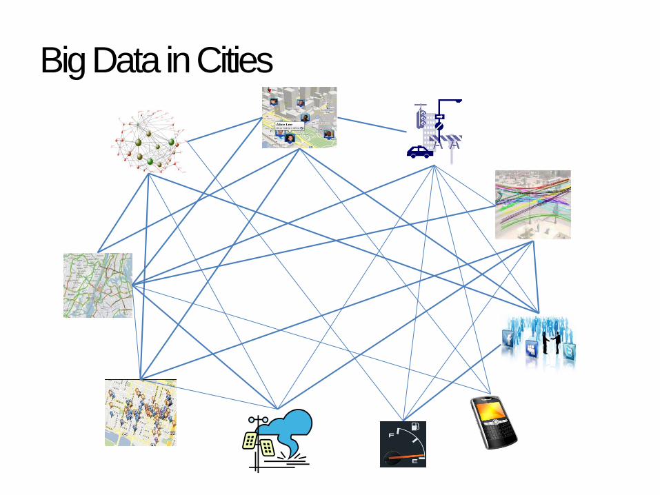
Big Data in Cities
Cities OSPeople
The Environment
Win
Win
Win
Urban
Computing
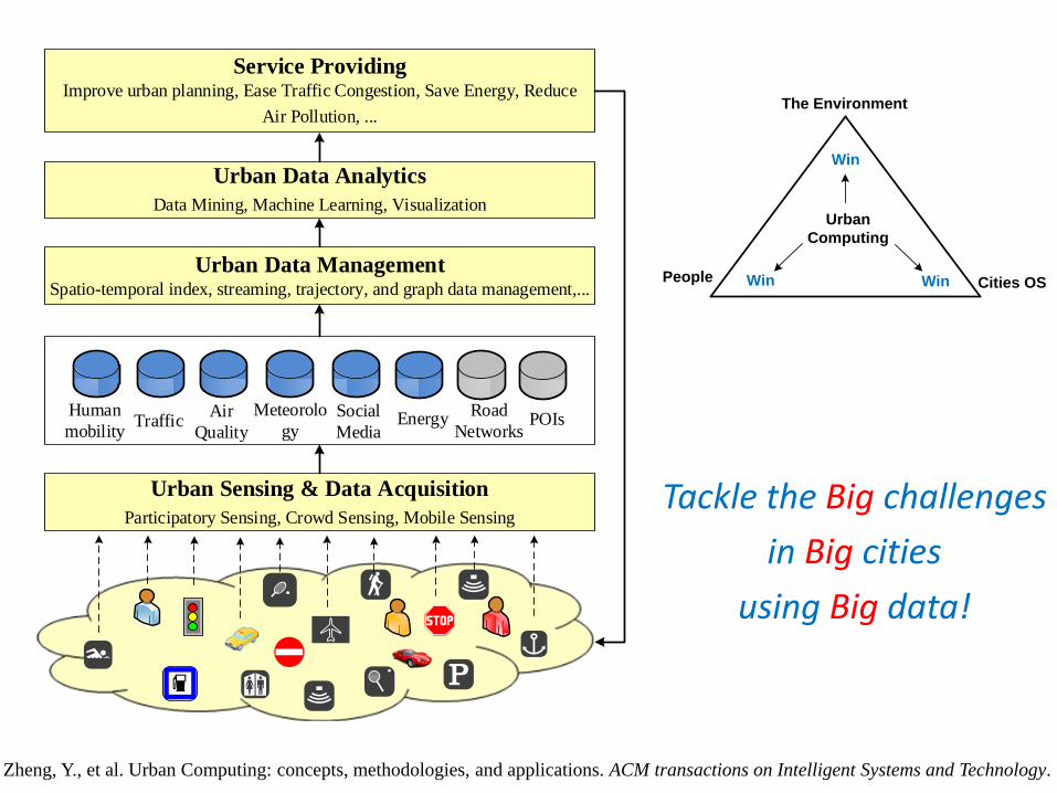
Tackle the Big challenges
in Big cities
using Big data!
Urban Sensing & Data Acquisition
Participatory Sensing, Crowd Sensing, Mobile Sensing
TrafficRoad
NetworksPOIsAir
Quality
Human
mobility
Meteorolo
gySocial
MediaEnergy
Urban Data ManagementSpatio-temporal index, streaming, trajectory, and graph data management,...
Urban Data Analytics
Data Mining, Machine Learning, Visualization
Service ProvidingImprove urban planning, Ease Traffic Congestion, Save Energy, Reduce
Air Pollution, ...
Zheng, Y., et al. Urban Computing: concepts, methodologies, and applications. ACM transactions on Intelligent Systems and Technology.
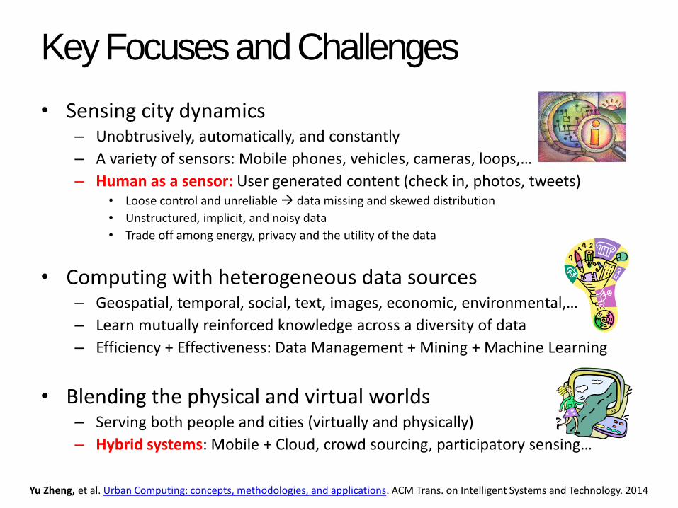
Key Focuses and Challenges
• Sensing city dynamics– Unobtrusively, automatically, and constantly
– A variety of sensors: Mobile phones, vehicles, cameras, loops,…
– Human as a sensor: User generated content (check in, photos, tweets)• Loose control and unreliable data missing and skewed distribution
• Unstructured, implicit, and noisy data
• Trade off among energy, privacy and the utility of the data
• Computing with heterogeneous data sources – Geospatial, temporal, social, text, images, economic, environmental,…
– Learn mutually reinforced knowledge across a diversity of data
– Efficiency + Effectiveness: Data Management + Mining + Machine Learning
• Blending the physical and virtual worlds– Serving both people and cities (virtually and physically)
– Hybrid systems: Mobile + Cloud, crowd sourcing, participatory sensing…
Yu Zheng, et al. Urban Computing: concepts, methodologies, and applications. ACM Trans. on Intelligent Systems and Technology. 2014
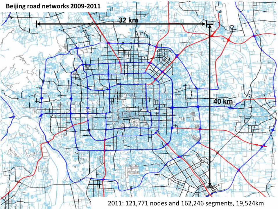
Beijing road networks 2009-2011
2011: 121,771 nodes and 162,246 segments, 19,524km
32 km
40 km
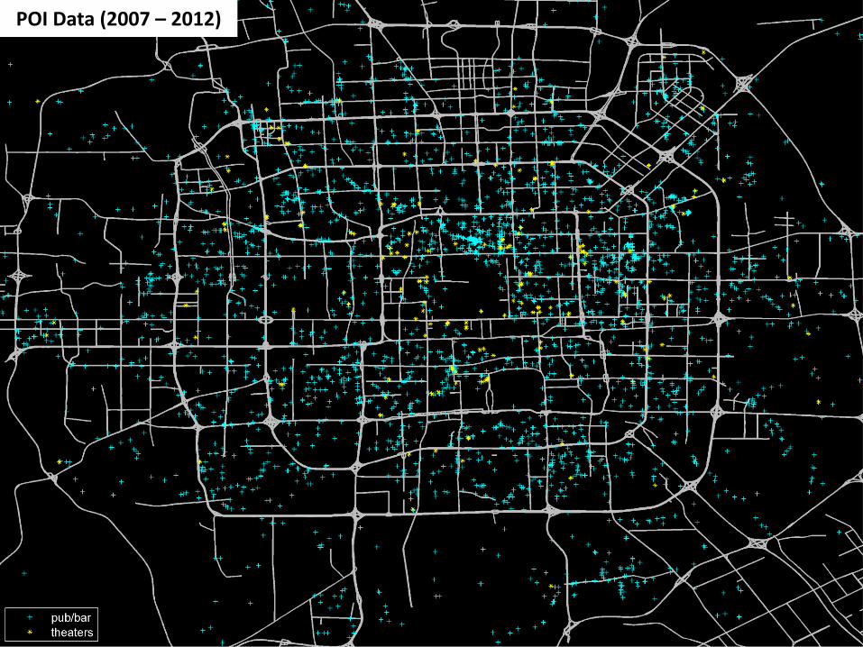
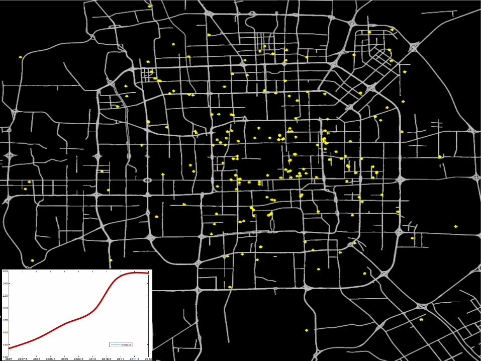
POI Data (2007 – 2012)
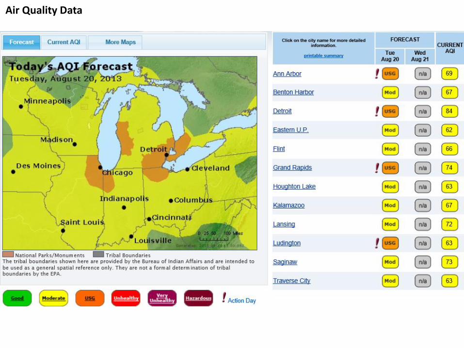
Air Quality Data
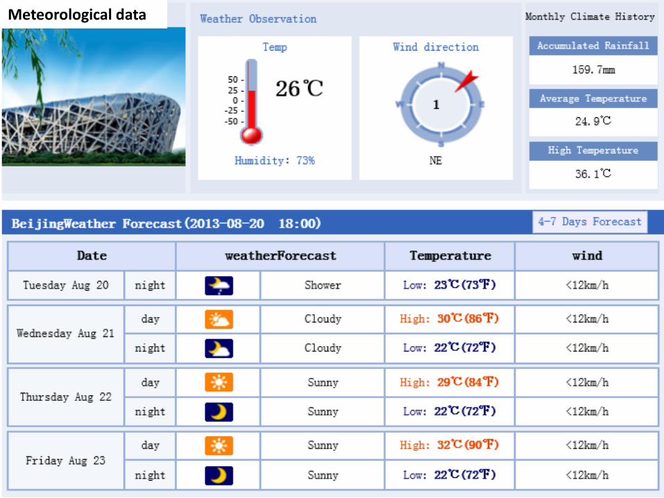
Meteorological data
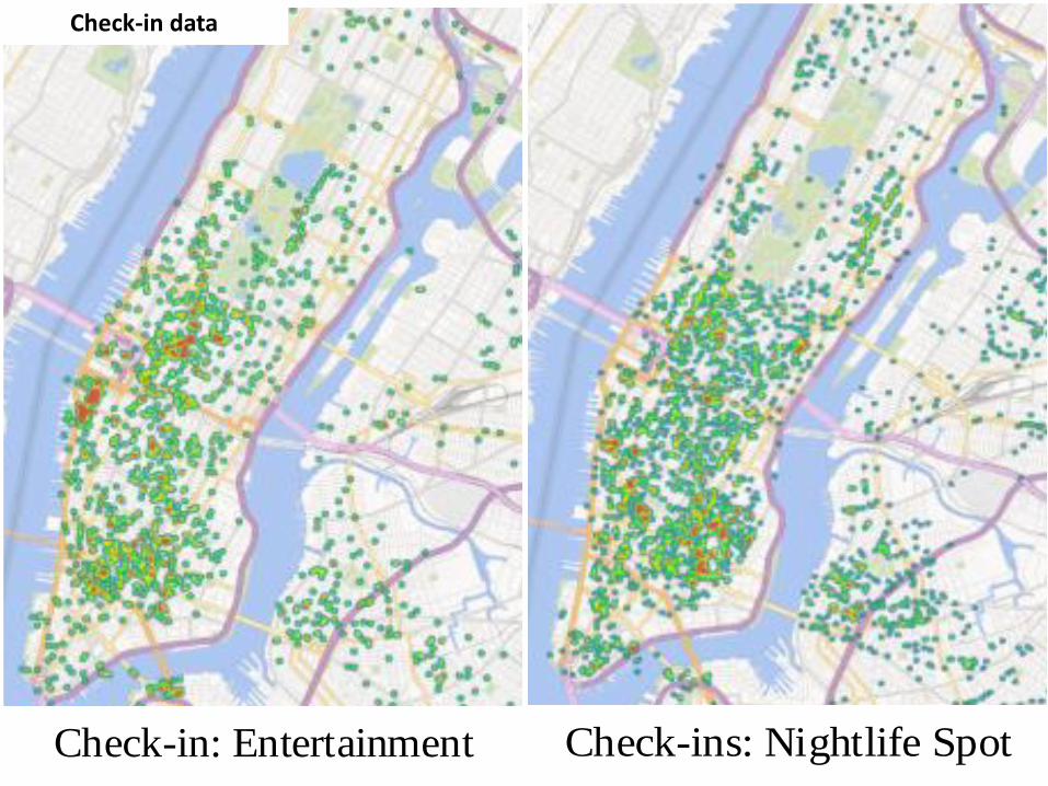
Check-in: Entertainment
Check-in data
Check-ins: Nightlife Spot
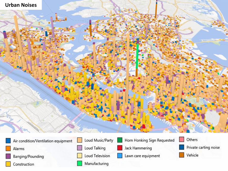
Urban Noises
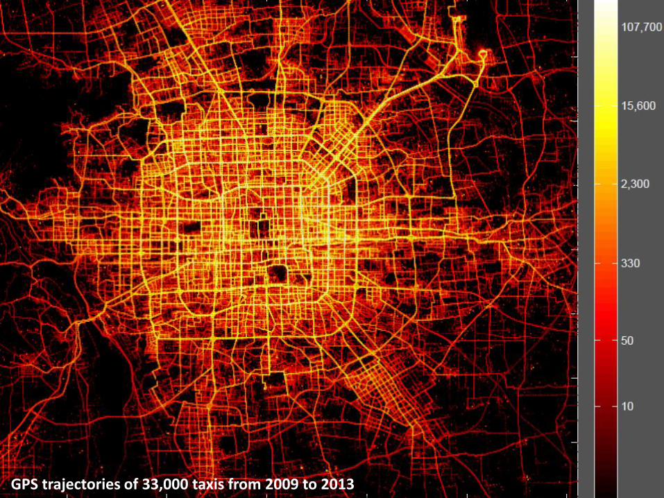
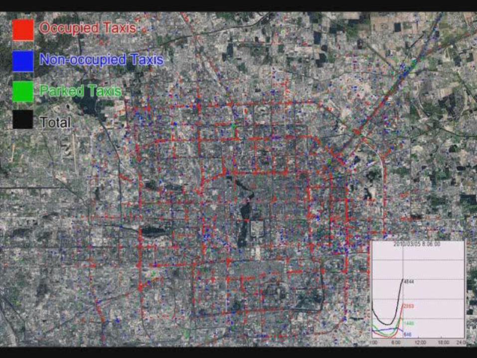
GPS trajectories of 33,000 taxis from 2009 to 2013
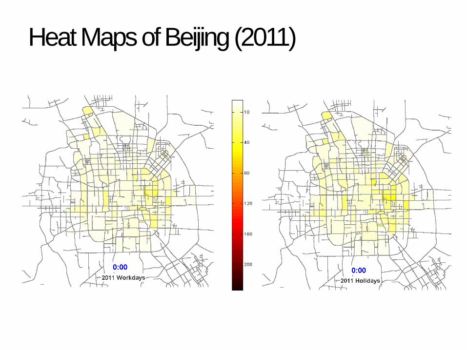
Heat Maps of Beijing (2011)
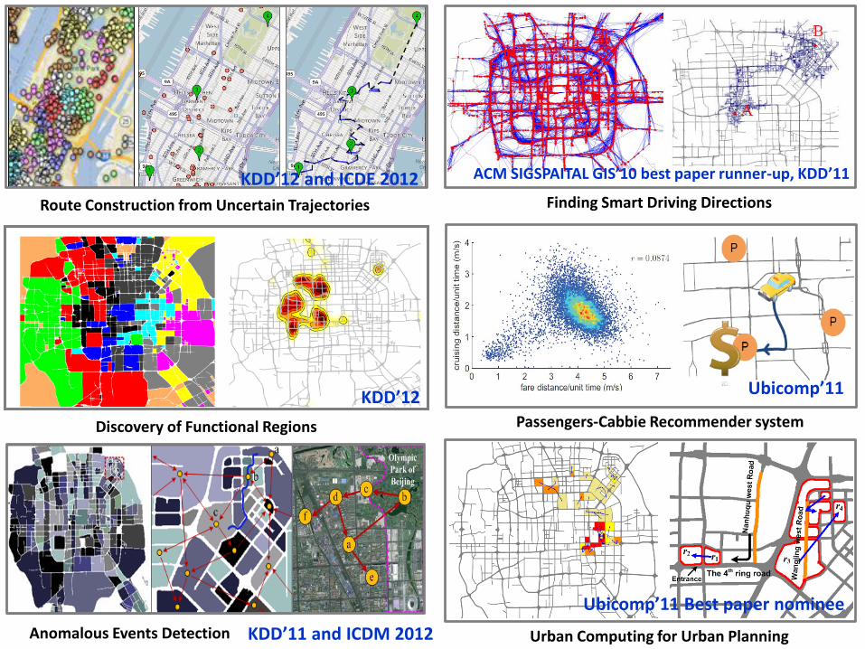
Finding Smart Driving Directions
ACM SIGSPAITAL GIS’10 best paper runner-up, KDD’11
Anomalous Events Detection KDD’11 and ICDM 2012
Passengers-Cabbie Recommender system
Ubicomp’11
Urban Computing for Urban Planning
Ubicomp’11 Best paper nominee
Discovery of Functional Regions
KDD’12
Route Construction from Uncertain Trajectories (a)
(b)
(c) (d) (e)
KDD’12 and ICDE 2012
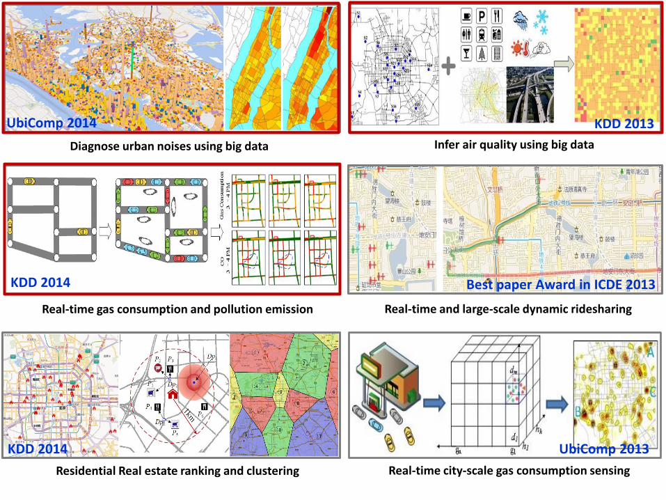
Real-time and large-scale dynamic ridesharing
Best paper Award in ICDE 2013
Infer air quality using big data
Real-time city-scale gas consumption sensing
KDD 2013
UbiComp 2013
UbiComp 2014
Diagnose urban noises using big data
Real-time gas consumption and pollution emission
KDD 2014
KDD 2014
Residential Real estate ranking and clustering
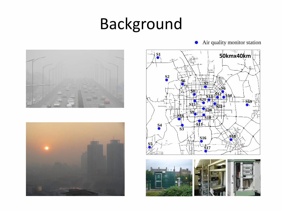
BackgroundAir quality monitor station
S1
S2
S4
S5
S8
S3
S6S7
S6
S9
S10
S12
S11
S13 S14
S22S15
S16
S16
S17
S18
S19
S20
S21
50kmx40km
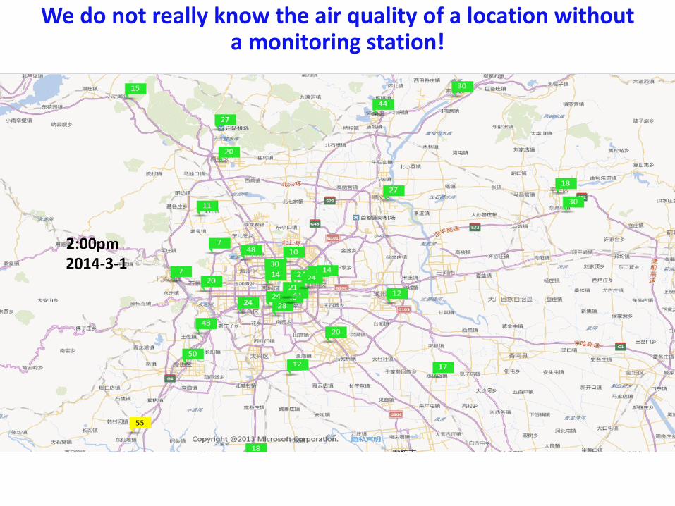
We do not really know the air quality of a location without a monitoring station!
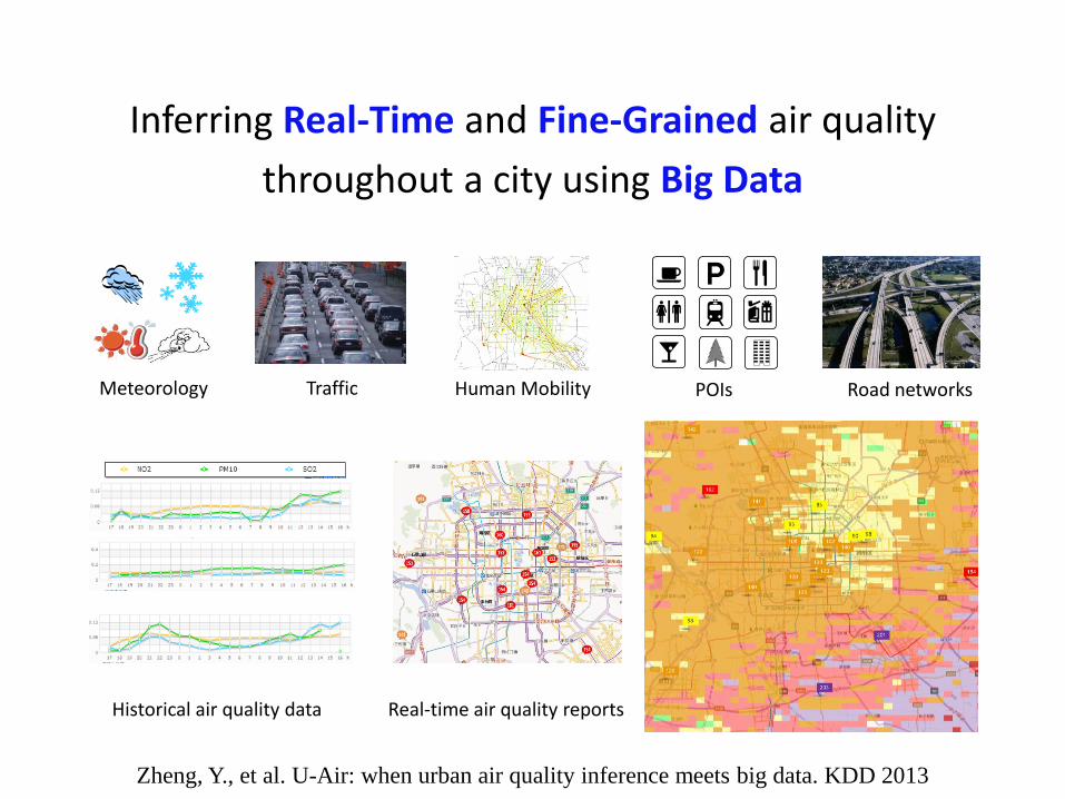
Inferring Real-Time and Fine-Grained air quality
throughout a city using Big Data
Meteorology Traffic POIs Road networksHuman Mobility
Historical air quality data Real-time air quality reports
Zheng, Y., et al. U-Air: when urban air quality inference meets big data. KDD 2013
S1
S2
S4
S5
S8
S3
S6S7
S6
S9
S10
S12
S11
S13 S14
S22S15
S16
S16
S17
S18
S19
S20
S21
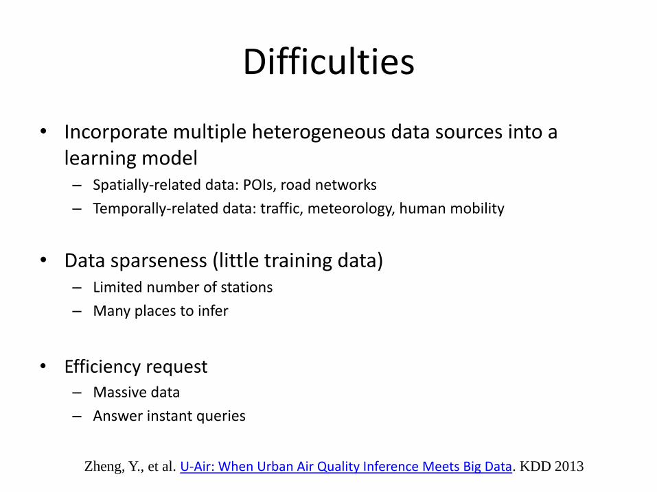
Difficulties
• Incorporate multiple heterogeneous data sources into a learning model– Spatially-related data: POIs, road networks
– Temporally-related data: traffic, meteorology, human mobility
• Data sparseness (little training data)– Limited number of stations
– Many places to infer
• Efficiency request – Massive data
– Answer instant queries
Zheng, Y., et al. U-Air: When Urban Air Quality Inference Meets Big Data. KDD 2013
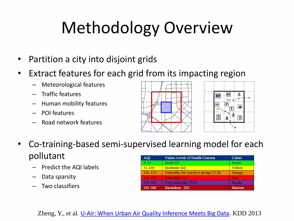
Methodology Overview
• Partition a city into disjoint grids
• Extract features for each grid from its impacting region– Meteorological features
– Traffic features
– Human mobility features
– POI features
– Road network features
• Co-training-based semi-supervised learning model for each pollutant– Predict the AQI labels
– Data sparsity
– Two classifiers
Zheng, Y., et al. U-Air: When Urban Air Quality Inference Meets Big Data. KDD 2013
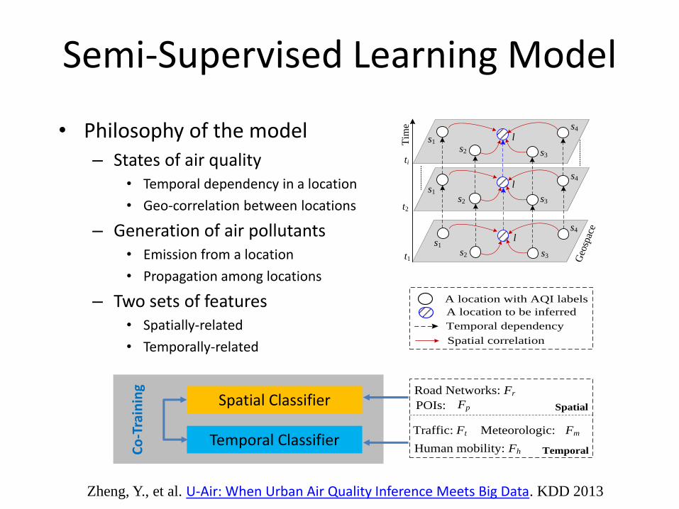
Semi-Supervised Learning Model
• Philosophy of the model– States of air quality
• Temporal dependency in a location
• Geo-correlation between locations
– Generation of air pollutants• Emission from a location
• Propagation among locations
– Two sets of features• Spatially-related
• Temporally-related
s2
s1
s3
s4
l
s2
s1
s3
s4l
s2
s1
s3
s4
ti
t1
t2
l
Tim
e
Geo
spac
e
A location with AQI labels
A location to be inferred
Temporal dependency
Spatial correlation
POIs: Spatial
Fh Temporal
Road Networks: Fr
Ft FmMeteorologic:Traffic:
Human mobility:
FpSpatial Classifier
Temporal Classifier
Co
-Tra
inin
g
Zheng, Y., et al. U-Air: When Urban Air Quality Inference Meets Big Data. KDD 2013
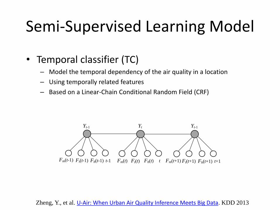
Semi-Supervised Learning Model
• Temporal classifier (TC)– Model the temporal dependency of the air quality in a location
– Using temporally related features
– Based on a Linear-Chain Conditional Random Field (CRF)
Yt-1
Fm(t-1) t-1Ft(t-1) Fh(t-1) Fm(t) tFt(t) Fh(t) Fm(t+1) t+1Ft(t+1) Fh(t+1)
Yt Yt-1
Zheng, Y., et al. U-Air: When Urban Air Quality Inference Meets Big Data. KDD 2013
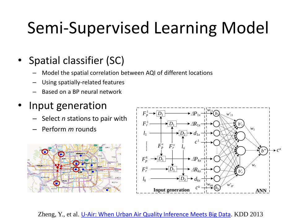
Semi-Supervised Learning Model
• Spatial classifier (SC)– Model the spatial correlation between AQI of different locations
– Using spatially-related features
– Based on a BP neural network
• Input generation– Select n stations to pair with
– Perform m rounds
∆P1x
∆R1x
c
D1Fp
Fr
l1 D2
c
d1x
D1
D2
D1
D1
1
1
Fp
Fr
lk
k
k
Fpx
Frx lx
∆Pkx
∆Rkx
c
dkx
1
k
x
ANNInput generation
w'11
w'qr
w1
wr
wpq
w11b1
bq
b'r
b'1
b''
∆P1x
∆R1x
c
D1Fp
Fr
l1 D2
c
d1x
D1
D2
D1
D1
1
1
Fp
Fr
lk
k
k
Fpx
Frx lx
∆Pkx
∆Rkx
c
dkx
1
k
x
ANNInput generation
w'11
w'qr
w1
wr
wpq
w11b1
bq
b'r
b'1
b''
Zheng, Y., et al. U-Air: When Urban Air Quality Inference Meets Big Data. KDD 2013
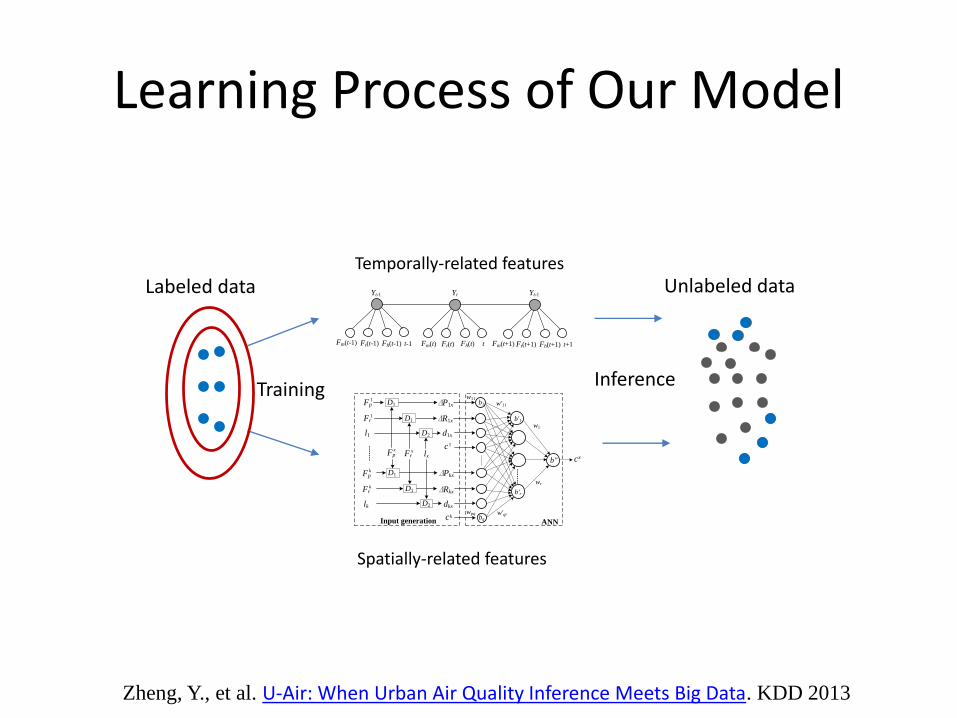
Learning Process of Our Model
Yt-1
Fm(t-1) t-1Ft(t-1) Fh(t-1) Fm(t) tFt(t) Fh(t) Fm(t+1) t+1Ft(t+1) Fh(t+1)
Yt Yt-1
∆P1x
∆R1x
c
D1Fp
Fr
l1 D2
c
d1x
D1
D2
D1
D1
1
1
Fp
Fr
lk
k
k
Fpx
Frx lx
∆Pkx
∆Rkx
c
dkx
1
k
x
ANNInput generation
w'11
w'qr
w1
wr
wpq
w11b1
bq
b'r
b'1
b''
Training
Temporally-related features
Spatially-related features
Labeled data Unlabeled data
Inference
Zheng, Y., et al. U-Air: When Urban Air Quality Inference Meets Big Data. KDD 2013
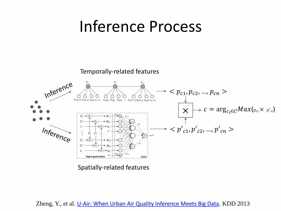
Inference Process
Yt-1
Fm(t-1) t-1Ft(t-1) Fh(t-1) Fm(t) tFt(t) Fh(t) Fm(t+1) t+1Ft(t+1) Fh(t+1)
Yt Yt-1
∆P1x
∆R1x
c
D1Fp
Fr
l1 D2
c
d1x
D1
D2
D1
D1
1
1
Fp
Fr
lk
k
k
Fpx
Frx lx
∆Pkx
∆Rkx
c
dkx
1
k
x
ANNInput generation
w'11
w'qr
w1
wr
wpq
w11b1
bq
b'r
b'1
b''
Temporally-related features
Spatially-related features
< 𝑝𝑐1, 𝑝𝑐2, …, 𝑝𝑐𝑛 >
< 𝑝′𝑐1, 𝑝′𝑐2, …, 𝑝′𝑐𝑛 >
× 𝑐 = arg𝑐𝑖∈𝒞𝑀𝑎𝑥(𝑝𝑐𝑖× 𝑝′𝑐𝑖)
Zheng, Y., et al. U-Air: When Urban Air Quality Inference Meets Big Data. KDD 2013
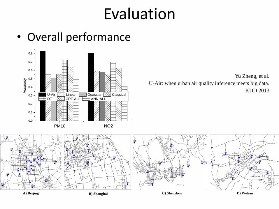
Evaluation
• Overall performance
0.0
0.1
0.2
0.3
0.4
0.5
0.6
0.7
0.8
NO2PM10
Accu
racy
U-Air Linear Guassian Classical
DT CRF-ALL ANN-ALL
Yu Zheng, et al.
U-Air: when urban air quality inference meets big data.
KDD 2013
S1
S2
S4
S5
S8
S5
S2
S1
S7
S5
S3
S3
S6S7
S6
S9
S10
S12
S11
S13 S14
S22S15
S16
S16
S17
S18
S19
S20
S21
S3
S7
S6
S4
S1
S8
S9
S10
S1
S4
S2
S6
S9
S8
S1
S2
S4
S3S10
S5
S9
S6 S7
S8
A) Beijing B) Shanghai C) Shenzhen D) Wuhan
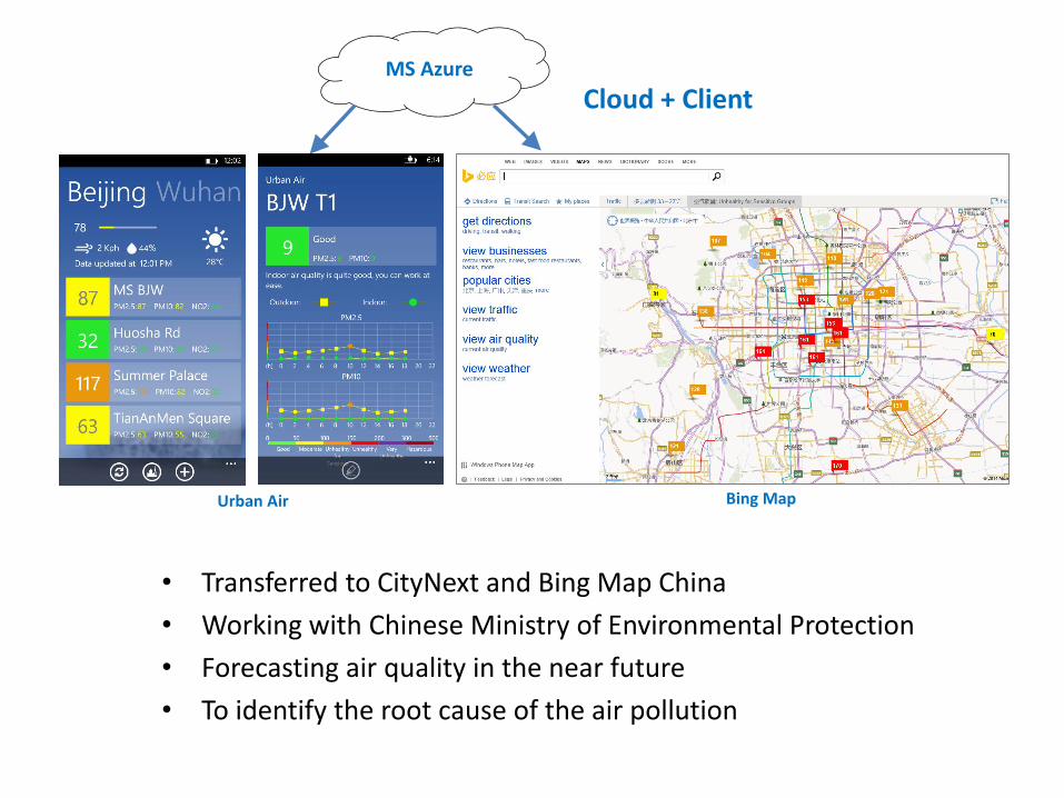
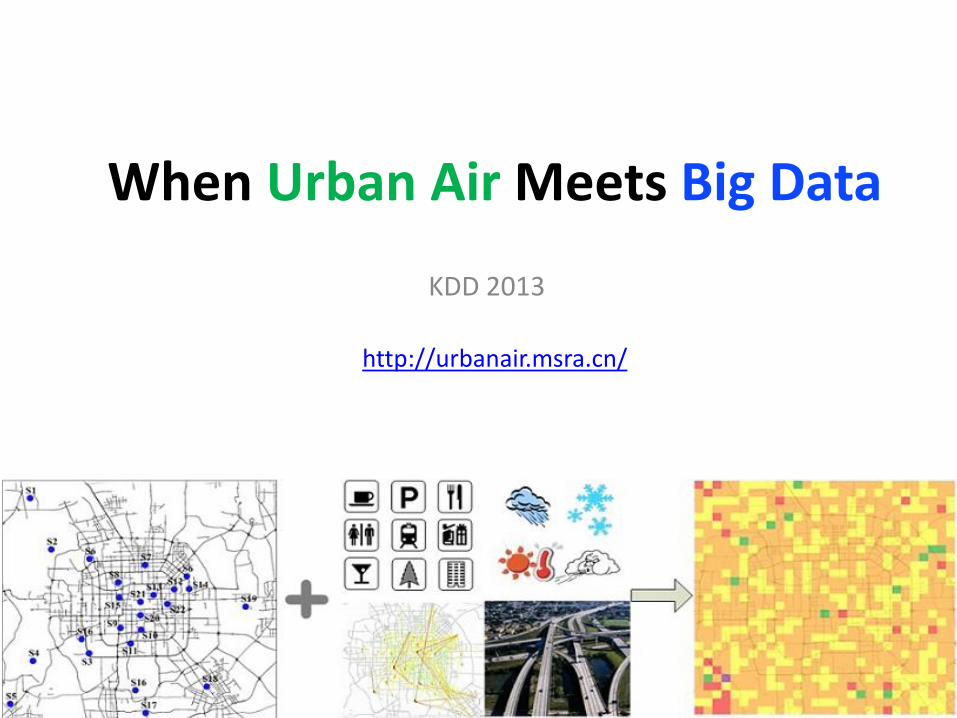
Cloud + ClientMS Azure
Urban Air
• Transferred to CityNext and Bing Map China
• Working with Chinese Ministry of Environmental Protection
• Forecasting air quality in the near future
• To identify the root cause of the air pollution
Bing Map
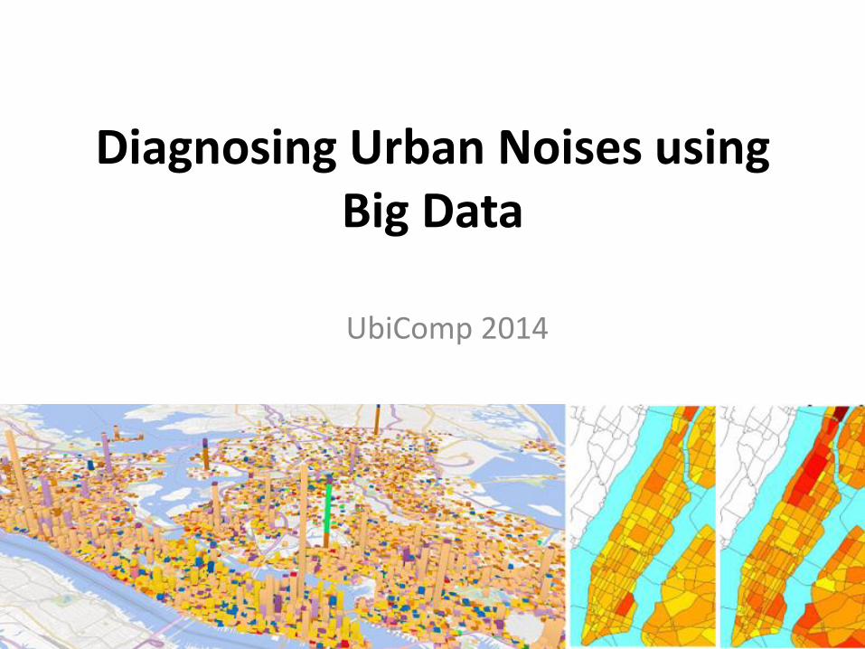
Diagnosing Urban Noises using Big Data
UbiComp 2014
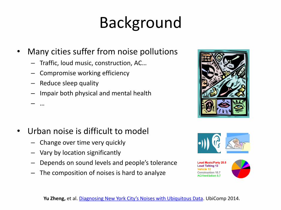
Background
• Many cities suffer from noise pollutions– Traffic, loud music, construction, AC…
– Compromise working efficiency
– Reduce sleep quality
– Impair both physical and mental health
– …
• Urban noise is difficult to model – Change over time very quickly
– Vary by location significantly
– Depends on sound levels and people’s tolerance
– The composition of noises is hard to analyze
Yu Zheng, et al. Diagnosing New York City’s Noises with Ubiquitous Data. UbiComp 2014.
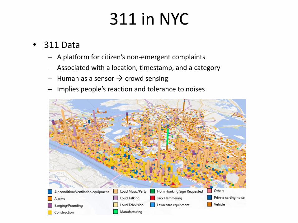
311 in NYC
• 311 Data– A platform for citizen’s non-emergent complaints
– Associated with a location, timestamp, and a category
– Human as a sensor crowd sensing
– Implies people’s reaction and tolerance to noises
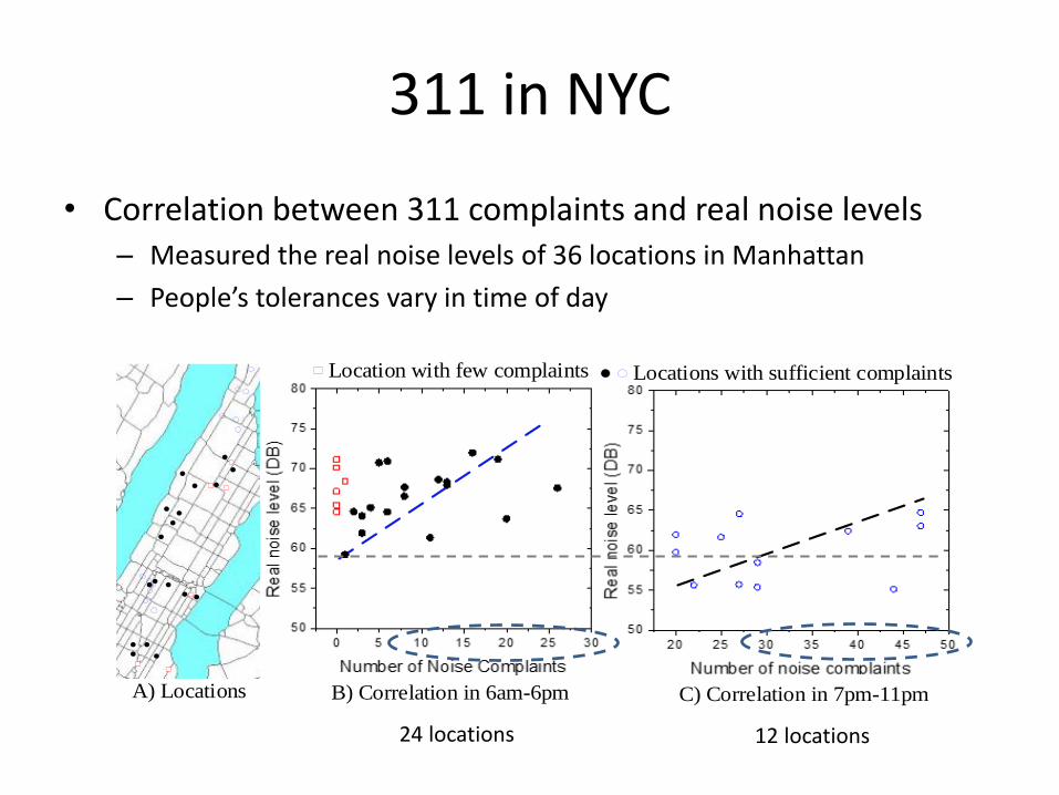
311 in NYC
• Correlation between 311 complaints and real noise levels– Measured the real noise levels of 36 locations in Manhattan
– People’s tolerances vary in time of day
Location with few complaints Locations with sufficient complaints
A) Locations B) Correlation in 6am-6pm C) Correlation in 7pm-11pm
24 locations 12 locations
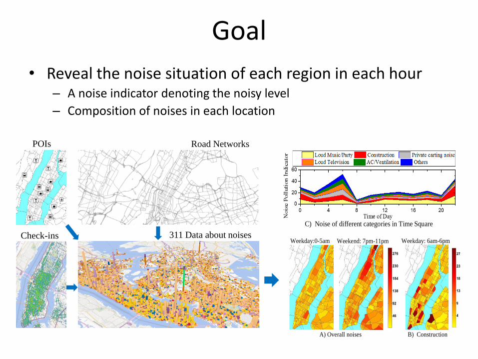
Goal
• Reveal the noise situation of each region in each hour– A noise indicator denoting the noisy level
– Composition of noises in each location
Road Networks
Check-in all
Check-ins
POIs
311 Data about noisesWeekday: 6am-6pmWeekend: 7pm-11pm
B) Construction
Weekday:0-5am
A) Overall noises
C) Noise of different categories in Time Square
Weekday: 6am-6pmWeekend: 7pm-11pm
B) Construction
Weekday:0-5am
A) Overall noises
C) Noise of different categories in Time Square
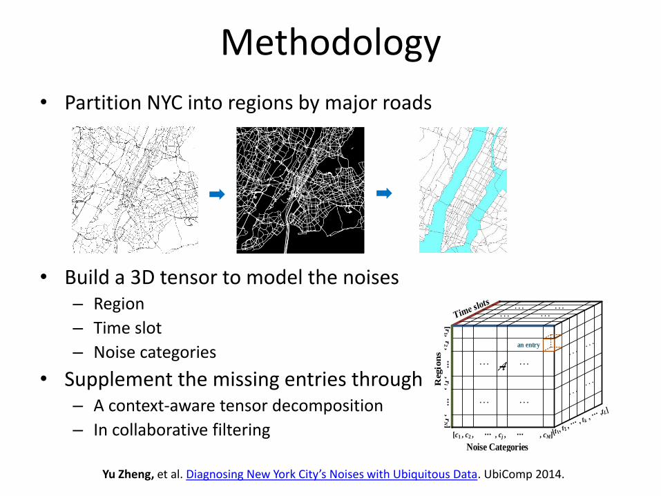
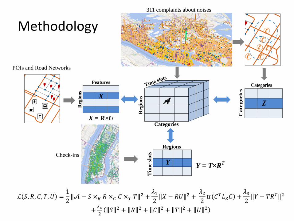
Methodology
• Partition NYC into regions by major roads
• Build a 3D tensor to model the noises– Region
– Time slot
– Noise categories
• Supplement the missing entries through– A context-aware tensor decomposition
– In collaborative filtering Noise Categories
Regio
ns
... ...... ...
... ...
......
[r1 , r
2 ,
, ri ,
, rN]
[c1 , c2 , , cj , , cM]
A
an entry
R
TS
C
N
dR
dC
dT
M
L
Yu Zheng, et al. Diagnosing New York City’s Noises with Ubiquitous Data. UbiComp 2014.
Methodology
Noise Categories
Regio
ns
... ...... ...
... ...
......
[r1 , r
2 ,
, ri ,
, rN]
[c1 , c2 , , cj , , cM]
A
an entry
R
TS
C
N
dR
dC
dT
M
L
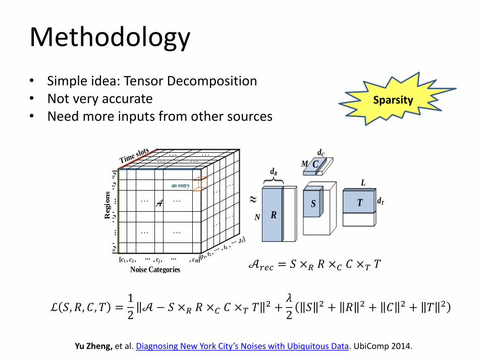
ℒ 𝑆, 𝑅, 𝐶, 𝑇 =1
2𝒜 − 𝑆 ×𝑅 𝑅 ×𝐶 𝐶 ×𝑇 𝑇
2 +𝜆
2𝑆 2 + 𝑅 2 + 𝐶 2 + 𝑇 2
𝒜𝑟𝑒𝑐 = 𝑆 ×𝑅 𝑅 ×𝐶 𝐶 ×𝑇 𝑇
• Simple idea: Tensor Decomposition• Not very accurate• Need more inputs from other sources
Sparsity
Yu Zheng, et al. Diagnosing New York City’s Noises with Ubiquitous Data. UbiComp 2014.
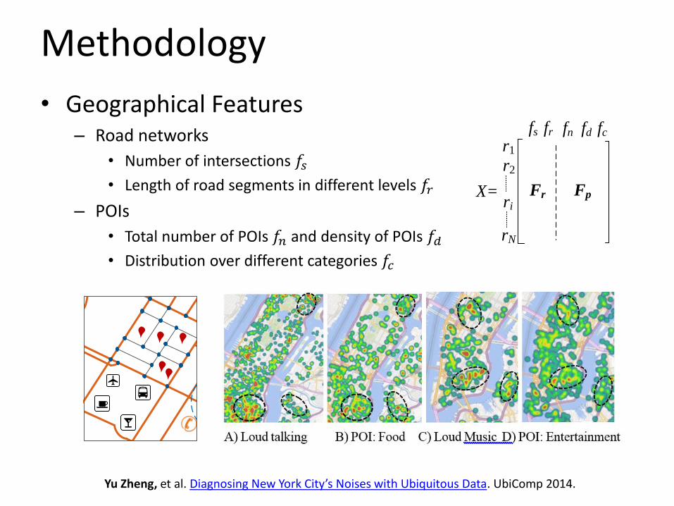
Methodology
• Geographical Features– Road networks
• Number of intersections 𝑓𝑠• Length of road segments in different levels 𝑓𝑟
– POIs
• Total number of POIs 𝑓𝑛 and density of POIs 𝑓𝑑• Distribution over different categories 𝑓𝑐
User check-in
Road intersection
311 complaint
POIs
Small streets
Major roads
r1
r2
fs fr fc
Fr Fp
rN
X=ri
fn fd
Yu Zheng, et al. Diagnosing New York City’s Noises with Ubiquitous Data. UbiComp 2014.
Methodology
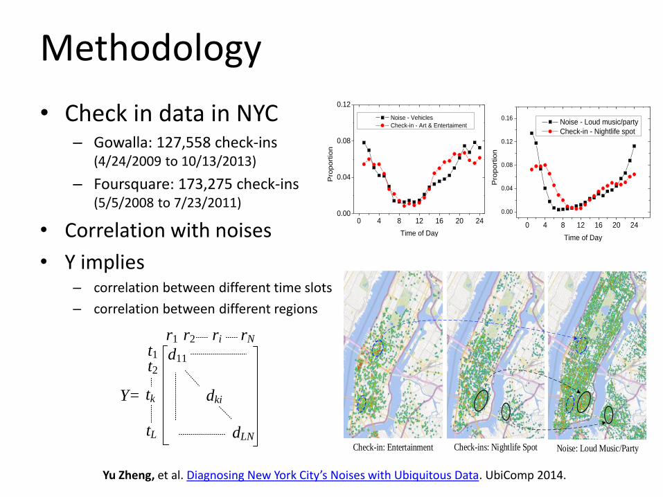
• Check in data in NYC– Gowalla: 127,558 check-ins
(4/24/2009 to 10/13/2013)
– Foursquare: 173,275 check-ins (5/5/2008 to 7/23/2011)
• Correlation with noises
• Y implies– correlation between different time slots
– correlation between different regions
Check-in: Entertainment Noise: Loud Music/PartyCheck-ins: Nightlife Spot
0 4 8 12 16 20 240.00
0.04
0.08
0.12
Pro
po
rtio
n
Time of Day
Noise - Vehicles
Check-in - Art & Entertaiment
0 4 8 12 16 20 24
0.00
0.04
0.08
0.12
0.16
Pro
po
rtio
n
Time of Day
Noise - Loud music/party
Check-in - Nightlife spot
r1 ri rN
t1
tL
tk
t2
Y=
r2
dki
dLN
d11
Yu Zheng, et al. Diagnosing New York City’s Noises with Ubiquitous Data. UbiComp 2014.
Methodology
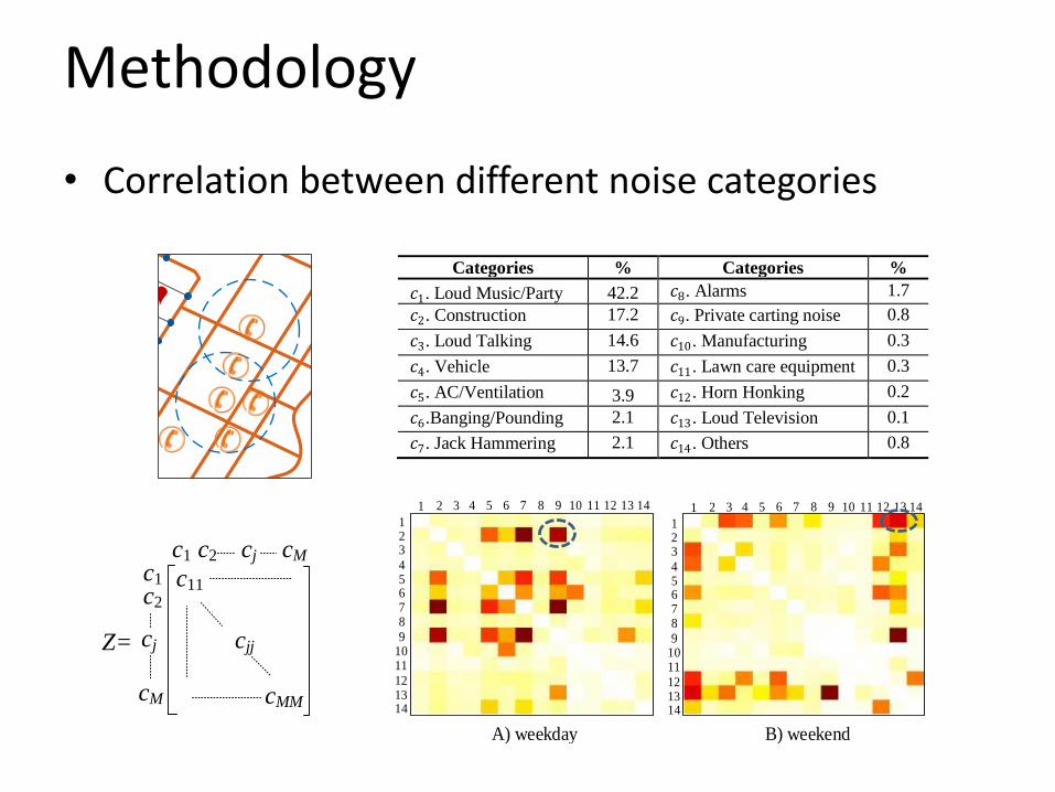
• Correlation between different noise categories
User check-in
Road intersection
311 complaint
POIs
Small streets
Major roads
123
45678
91011
121314
1 2 3 4 5 6 7 8 9 10 11 12 13 14
A) weekday B) weekend
123
45678
91011
121314
1 2 3 4 5 6 7 8 9 10 11 12 13 14
Categories % Categories %
𝑐1. Loud Music/Party 42.2 𝑐8. Alarms 1.7
𝑐2. Construction 17.2 𝑐9. Private carting noise 0.8
𝑐3. Loud Talking 14.6 𝑐10. Manufacturing 0.3
𝑐4. Vehicle 13.7 𝑐11. Lawn care equipment 0.3
𝑐5. AC/Ventilation equipment
3.9 𝑐12. Horn Honking 0.2
𝑐6.Banging/Pounding 2.1 𝑐13. Loud Television 0.1
𝑐7. Jack Hammering 2.1 𝑐14. Others 0.8
c1 cj cM
c1
cM
cj
c2
Z=
c2
cjj
cMM
c11
Methodology
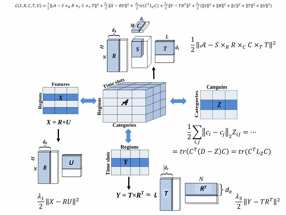
ℒ 𝑆, 𝑅, 𝐶, 𝑇, 𝑈 =1
2𝒜 − 𝑆 ×𝑅 𝑅 ×𝐶 𝐶 ×𝑇 𝑇
2 +𝜆12𝑋 − 𝑅𝑈 2 +
𝜆22tr 𝐶𝑇𝐿𝑍𝐶 +
𝜆32𝑌 − 𝑇𝑅𝑇 2
+𝜆4
2𝑆 2 + 𝑅 2 + 𝐶 2 + 𝑇 2 + 𝑈 2
Categories
Regio
ns
A
Tim
e sl
ots
Regions
Y
Y = T×RT
Check-ins
Check-in all
Categories
Cate
gorie
s
Z
User check-in
Road intersection
311 complaint
POIs
Small streets
Major roads
Reg
ion
sFeatures
X
User check-in
Road intersection
311 complaint
POIs
Small streets
Major roads
POIs and Road Networks
Y = T×RT
X = R×U
311 complaints about noises
Categories
Regio
nsA
Tim
e sl
ots
Regions
Y
Y = T×RT
Categories
Cate
gorie
s
ZReg
ion
s
Features
X
1
2
𝑖,𝑗
𝑐𝑖 − 𝑐𝑗 2𝑍𝑖𝑗 = ⋯
= 𝑡𝑟 𝐶𝑇 𝐷 − 𝑍 𝐶 = 𝑡𝑟(𝐶𝑇𝐿𝑍𝐶)
X = R×U
Noise Categories
Regio
ns
... ...... ...
... ...
......
[r1 , r
2 ,
, ri ,
, rN]
[c1 , c2 , , cj , , cM]
A
an entry
R
TS
C
N
dR
dC
dT
M
L
Noise Categories
Regio
ns
... ...... ...
... ...
......
[r1 , r
2 ,
, ri ,
, rN]
[c1 , c2 , , cj , , cM]
A
an entry
R
TS
C
N
dR
dC
dT
M
L
U
𝜆12𝑋 − 𝑅𝑈 2
Y = T×RT
Noise Categories
Regio
ns
... ...... ...
... ...
......
[r1 , r
2 ,
, ri ,
, rN]
[c1 , c2 , , cj , , cM]
A
an entry
R
TS
C
N
dR
dC
dT
M
L
TL
Noise Categories
Regio
ns
... ...... ...
... ...
......
[r1 , r
2 ,
, ri ,
, rN]
[c1 , c2 , , cj , , cM]
A
an entry
R
TS
C
N
dR
dC
dT
M
L
Noise C
ategories
Regions
......
......
......
......
[r1, r2 , , ri , , rN]
[c1 , c
2 , , c
j , , c
M]
A
an en
try
R
TS C
N
dR
dC
dT
M
L
RTN
dR≈ 𝜆32𝑌 − 𝑇𝑅𝑇 2
ℒ 𝑆, 𝑅, 𝐶, 𝑇, 𝑈 =1
2𝒜 − 𝑆 ×𝑅 𝑅 ×𝐶 𝐶 ×𝑇 𝑇
2 +𝜆1
2𝑋 − 𝑅𝑈 2 +
𝜆2
2tr 𝐶𝑇𝐿𝑍𝐶 +
𝜆3
2𝑌 − 𝑇𝑅𝑇 2 +
𝜆4
2𝑆 2 + 𝑅 2 + 𝐶 2 + 𝑇 2 + 𝑈 2
Noise Categories
Regio
ns
... ...... ...
... ...
......
[r1 , r
2 ,
, ri ,
, rN]
[c1 , c2 , , cj , , cM]
A
an entry
R
TS
C
N
dR
dC
dT
M
L 1
2𝒜 − 𝑆 ×𝑅 𝑅 ×𝐶 𝐶 ×𝑇 𝑇
2
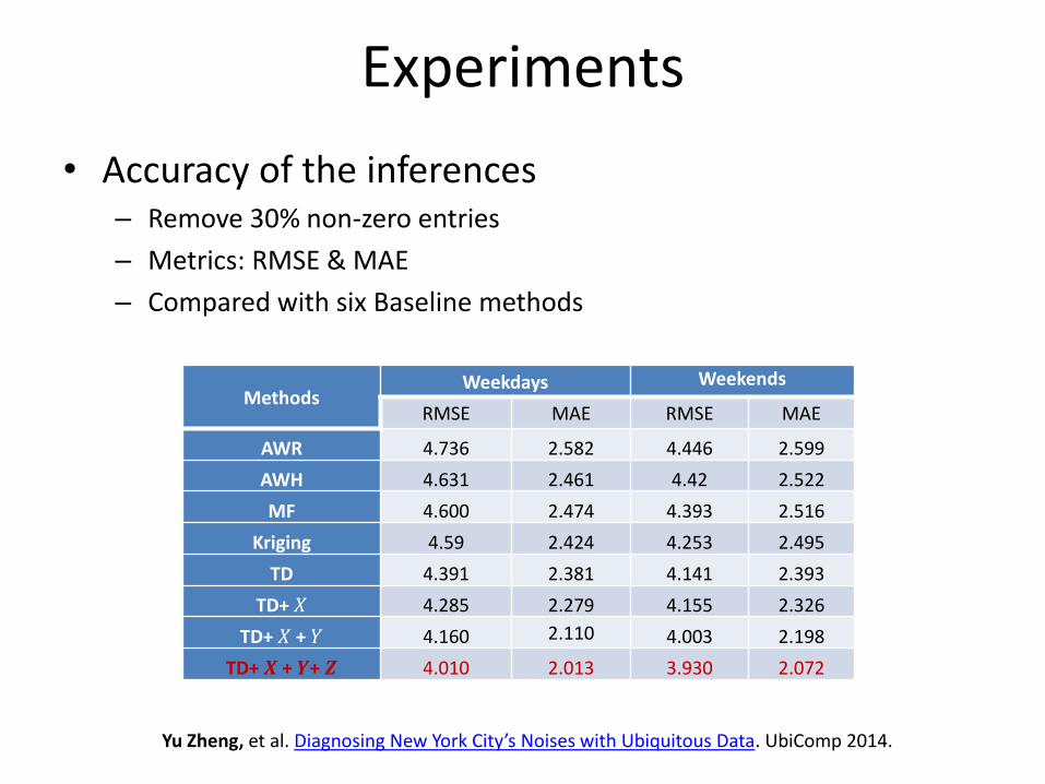
Experiments
MethodsWeekdays Weekends
RMSE MAE RMSE MAE
AWR 4.736 2.582 4.446 2.599
AWH 4.631 2.461 4.42 2.522
MF 4.600 2.474 4.393 2.516
Kriging 4.59 2.424 4.253 2.495
TD 4.391 2.381 4.141 2.393
TD+ 𝑋 4.285 2.279 4.155 2.326
TD+ 𝑋 + 𝑌 4.160 2.110 4.003 2.198
TD+ 𝑿 + 𝒀+ 𝒁 4.010 2.013 3.930 2.072
• Accuracy of the inferences– Remove 30% non-zero entries
– Metrics: RMSE & MAE
– Compared with six Baseline methods
Yu Zheng, et al. Diagnosing New York City’s Noises with Ubiquitous Data. UbiComp 2014.
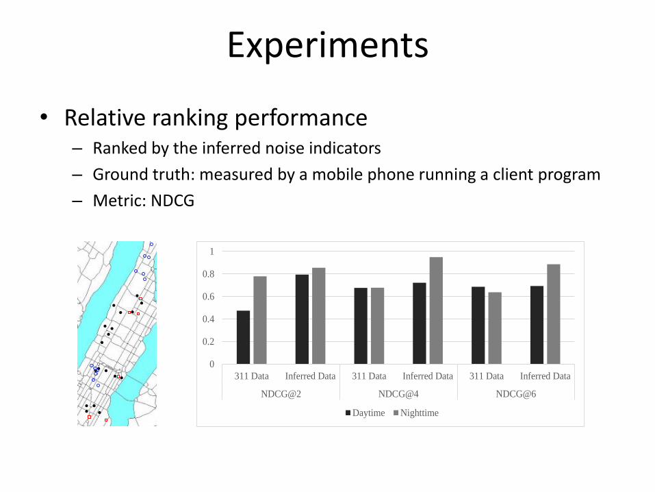
Experiments
• Relative ranking performance– Ranked by the inferred noise indicators
– Ground truth: measured by a mobile phone running a client program
– Metric: NDCG
0
0.2
0.4
0.6
0.8
1
311 Data Inferred Data 311 Data Inferred Data 311 Data Inferred Data
NDCG@2 NDCG@4 NDCG@6
Daytime Nighttime
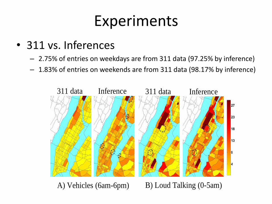
Experiments
• 311 vs. Inferences– 2.75% of entries on weekdays are from 311 data (97.25% by inference)
– 1.83% of entries on weekends are from 311 data (98.17% by inference)
0-6am
311 data Inference
B) Loud Talking (0-5am)A) Vehicles (6am-6pm)
311 data Inference
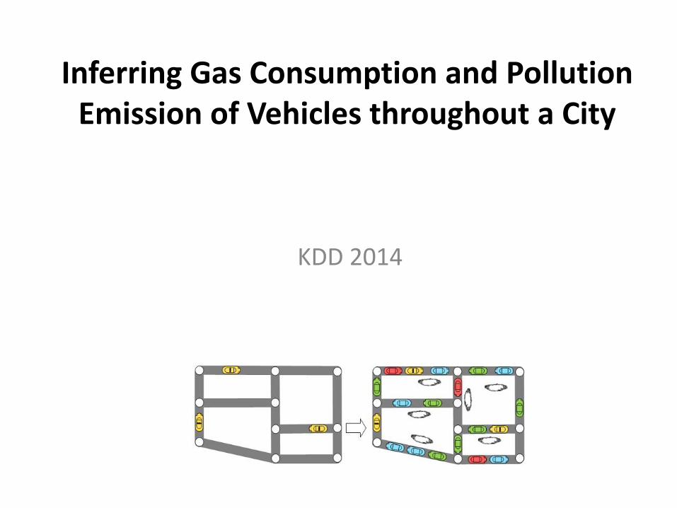
Inferring Gas Consumption and Pollution Emission of Vehicles throughout a City
KDD 2014
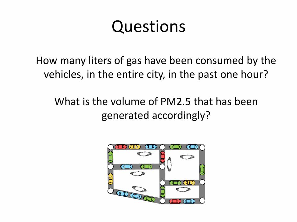
Questions
How many liters of gas have been consumed by the vehicles, in the entire city, in the past one hour?
What is the volume of PM2.5 that has been generated accordingly?
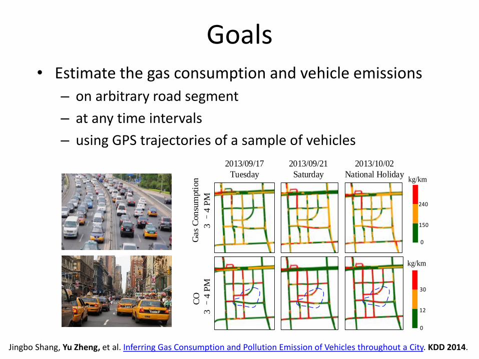
Goals• Estimate the gas consumption and vehicle emissions
– on arbitrary road segment
– at any time intervals
– using GPS trajectories of a sample of vehicles
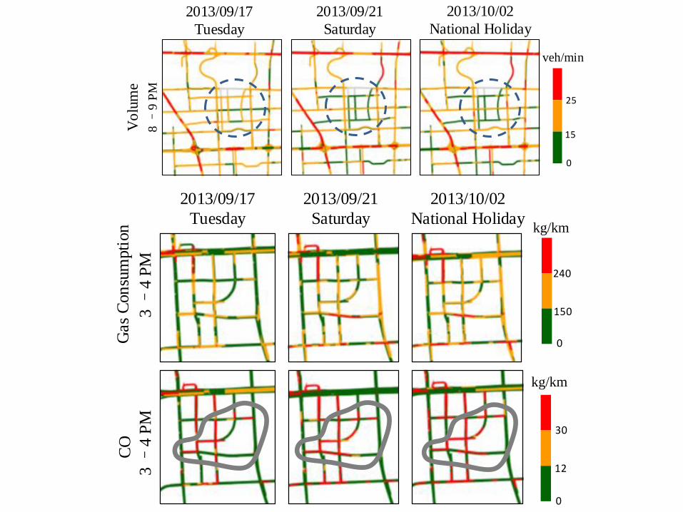
0
150
240
kg/km
3 –
4 P
M
Gas
Con
sum
pti
on
2013/09/17
Tuesday
2013/09/21
Saturday
2013/10/02
National Holiday
0
kg/km
12
30
CO
3 –
4 P
M
Jingbo Shang, Yu Zheng, et al. Inferring Gas Consumption and Pollution Emission of Vehicles throughout a City. KDD 2014.
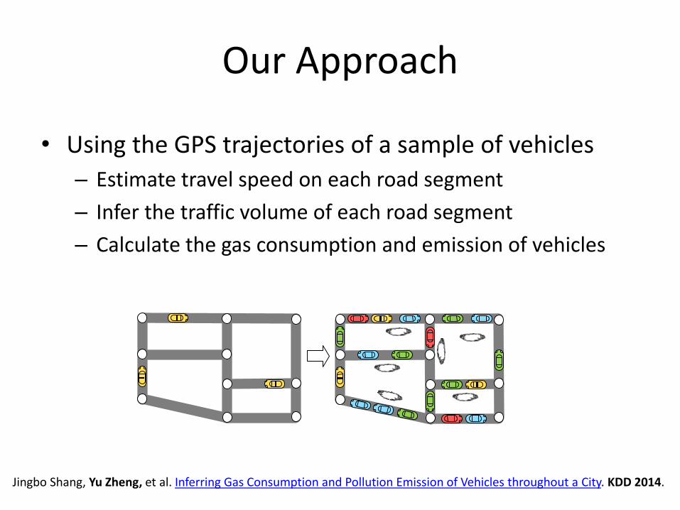
Our Approach
• Using the GPS trajectories of a sample of vehicles
– Estimate travel speed on each road segment
– Infer the traffic volume of each road segment
– Calculate the gas consumption and emission of vehicles
Jingbo Shang, Yu Zheng, et al. Inferring Gas Consumption and Pollution Emission of Vehicles throughout a City. KDD 2014.
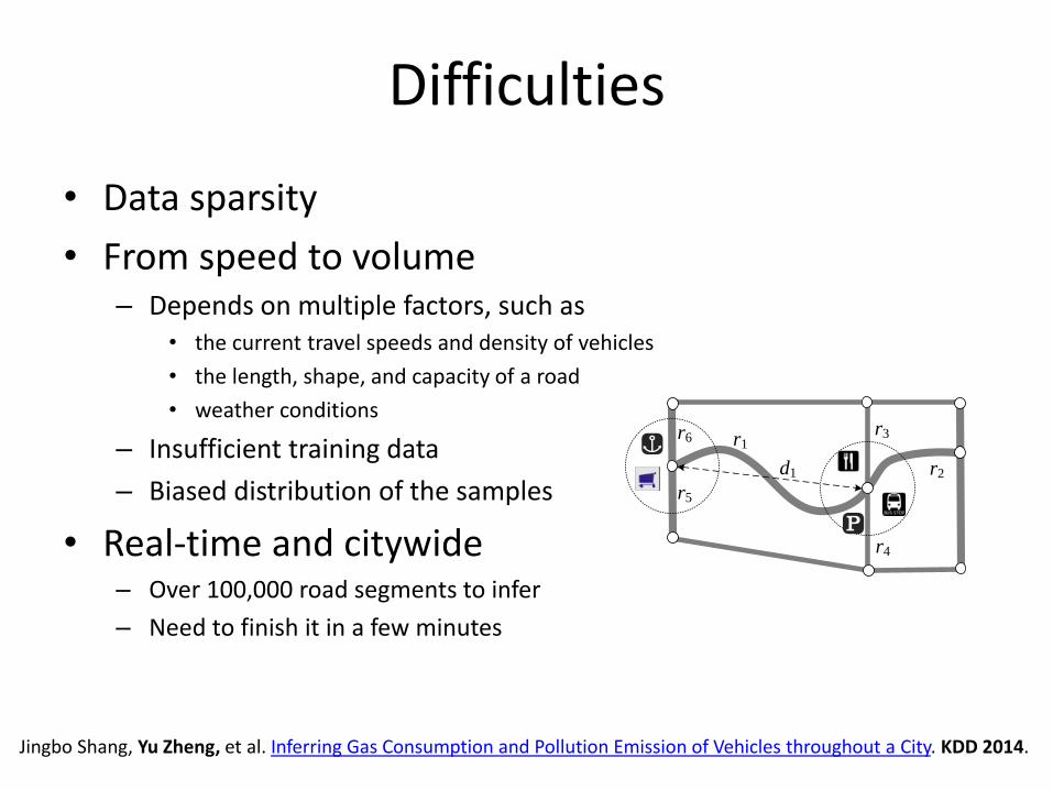
Difficulties
• Data sparsity
• From speed to volume– Depends on multiple factors, such as
• the current travel speeds and density of vehicles
• the length, shape, and capacity of a road
• weather conditions
– Insufficient training data
– Biased distribution of the samples
• Real-time and citywide– Over 100,000 road segments to infer
– Need to finish it in a few minutes
r1
d1 r2
r3
r4
r6
r5
Jingbo Shang, Yu Zheng, et al. Inferring Gas Consumption and Pollution Emission of Vehicles throughout a City. KDD 2014.
r2
Tr1
r3
r1
p1 p2
r4
p3
r2
r3
r1
v1 v2
r4
v3
v4 v4
v6 v5
v7
Tr2 Tr3
r1: (v1, v2, v4) r2: (v4, v5, v6) r3: (v5, v7) r4: (v2, v3)
v5
r1
d1 r2
r3
r4
r6
r5
r1
r2
rn
f1 f2 fk
Z
fr fp fg
g1 g2 g3 g16ti
ti+1
219
42
00 0 0
6 17
0 0 0tj 0
014
g1 g2 g3
g16
g4
g5 g6 g7 g8
g9 R10 g11 g12
g13 g14 g15
g1 g2 g3 g16
t1 22
0420
35
110
0
0 0 0
16 8
0 00 15
0 31
0
tn
0
0
0
0
27
tj
ti
t2
0 0 0 7 0
MG=
=M G
r1 r2 rnti
ti+1
tj
M r Mr
r1 r2 rng1 g2 g16
ti
ti+1
tj
M G MG
g1 g2 g16
Y X ZY
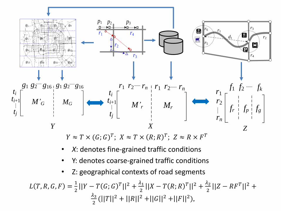
• X: denotes fine-grained traffic conditions
• Y: denotes coarse-grained traffic conditions
• Z: geographical contexts of road segments
𝑌 ≈ 𝑇 × (𝐺; 𝐺)𝑇; 𝑋 ≈ 𝑇 × 𝑅;𝑅 𝑇; 𝑍 ≈ 𝑅 × 𝐹𝑇
𝐿 𝑇, 𝑅, 𝐺, 𝐹 =1
2|𝑌 − 𝑇 𝐺; 𝐺 𝑇| 2 +
𝜆1
2|𝑋 − 𝑇 𝑅; 𝑅 𝑇| 2 +
𝜆2
2|𝑍 − 𝑅𝐹𝑇| 2 +
𝜆3
2( |𝑇 |2 + |𝑅| 2 + |𝐺 |2 + |𝐹 |2),
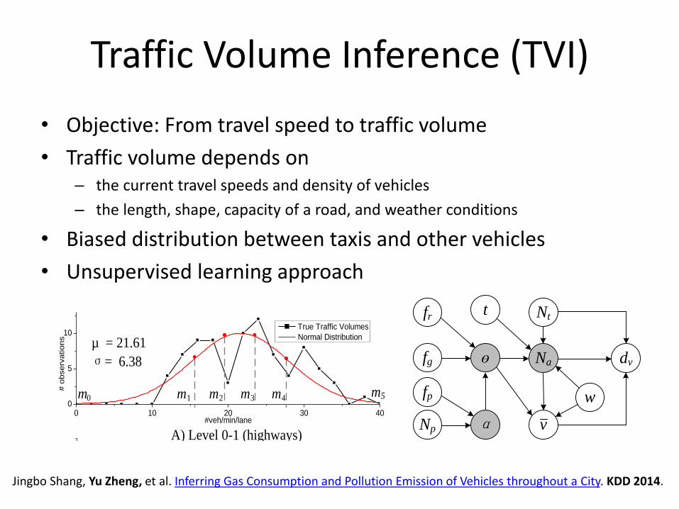
Traffic Volume Inference (TVI)
• Objective: From travel speed to traffic volume
• Traffic volume depends on– the current travel speeds and density of vehicles
– the length, shape, capacity of a road, and weather conditions
• Biased distribution between taxis and other vehicles
• Unsupervised learning approach
Jingbo Shang, Yu Zheng, et al. Inferring Gas Consumption and Pollution Emission of Vehicles throughout a City. KDD 2014.
fp
fg
t Nt
ɵ Na
v
dv
fr
w
Np α 0 10 20 30 40
0
5
10
# o
bserv
ations
#veh/min/lane
True Traffic Volumes
Normal Distributionµ = 21.61
σ= 6.38
0 10 20 30 400
10
20
30
40
# o
bserv
ations
#veh/min/lane
True Traffic Volumes
Normal Distribution
µ = 5.44
σ= 3.13
0 10 20 30 400
5
10
15
# o
bserv
ations
#veh/min/lane
True Traffic Volumes
Normal Distribution
µ = 2.95
σ= 2.38
A) Level 0-1 (highways)
B) Level 2 (main roads)
m1 m2 m3 m4m5 m 0
C) Level 3 (small streets)
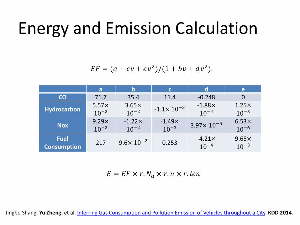
Energy and Emission Calculation
a b c d eCO 71.7 35.4 11.4 -0.248 0
Hydrocarbon5.57×10−2
3.65×10⁻²
-1.1× 10⁻³-1.88×10⁻⁴
1.25×10−5
Nox9.29×10−2
-1.22×10⁻²
-1.49×10⁻³
3.97× 10−56.53×10−6
Fuel Consumption
217 9.6× 10⁻² 0.253-4.21×10⁻⁴
9.65×10⁻³
𝐸𝐹 = (𝑎 + 𝑐𝑣 + 𝑒𝑣2)/(1 + 𝑏𝑣 + 𝑑𝑣2).
𝐸 = 𝐸𝐹 × 𝑟. 𝑁𝑎 × 𝑟. 𝑛 × 𝑟. 𝑙𝑒𝑛
Jingbo Shang, Yu Zheng, et al. Inferring Gas Consumption and Pollution Emission of Vehicles throughout a City. KDD 2014.
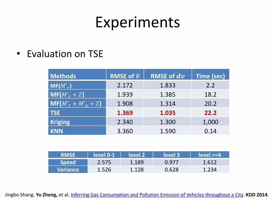
Experiments
Methods RMSE of 𝒗 RMSE of 𝒅𝒗 Time (sec)
MF(𝑀′𝑟) 2.172 1.833 2.2
MF(𝑀′𝑟 + 𝑍) 1.939 1.385 18.2
MF(𝑀′𝑟 +𝑀′𝑔 + 𝑍) 1.908 1.314 20.2
TSE 1.369 1.035 22.2
Kriging 2.340 1.300 1,000
KNN 3.360 1.590 0.14
• Evaluation on TSE
RMSE level 0-1 level 2 level 3 level >=4Speed 2.575 1.189 0.977 1.612
Variance 1.526 1.128 0.628 1.234
Jingbo Shang, Yu Zheng, et al. Inferring Gas Consumption and Pollution Emission of Vehicles throughout a City. KDD 2014.
Experiments
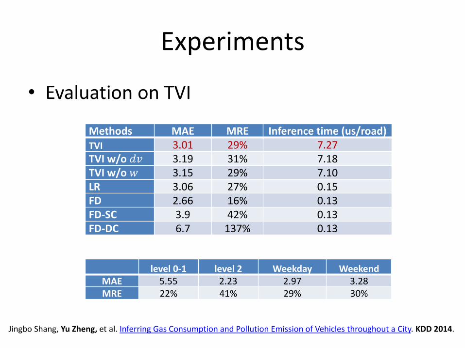
Methods MAE MRE Inference time (us/road)TVI 3.01 29% 7.27 TVI w/o 𝑑𝑣 3.19 31% 7.18TVI w/o 𝑤 3.15 29% 7.10LR 3.06 27% 0.15FD 2.66 16% 0.13FD-SC 3.9 42% 0.13FD-DC 6.7 137% 0.13
• Evaluation on TVI
level 0-1 level 2 Weekday WeekendMAE 5.55 2.23 2.97 3.28MRE 22% 41% 29% 30%
Jingbo Shang, Yu Zheng, et al. Inferring Gas Consumption and Pollution Emission of Vehicles throughout a City. KDD 2014.

Time 7:00 ~ 10:00 10:00~16:00 16:00~20:00 after 20:00 total
Level 0,1 2 3 0,1 2 3 0,1 2 3 0,1 2 3Holiday 0 0 0 6 14 4 6 8 1 4 6 0 49
Workday 7 28 8 29 74 9 28 92 7 6 17 4 309Total 43 136 142 37 358
Online components Time Offline components Time
Map-matching 4.94min Geo-feature extraction 149s
TSE 22.2s Historical pattern extraction 240s
TVI (inference) 0.84s TVI learning 89s
Total 5.32min Total 478s
• Efficiency
0
15
25
veh/min
8 –
9 P
M
Vo
lum
e
2013/09/17
Tuesday
2013/09/21
Saturday
2013/10/02
National Holiday
0
150
240
kg/km
3 –
4 P
M
Gas
Con
sum
pti
on
2013/09/17
Tuesday
2013/09/21
Saturday
2013/10/02
National Holiday
0
kg/km
12
30
CO
3 –
4 P
M
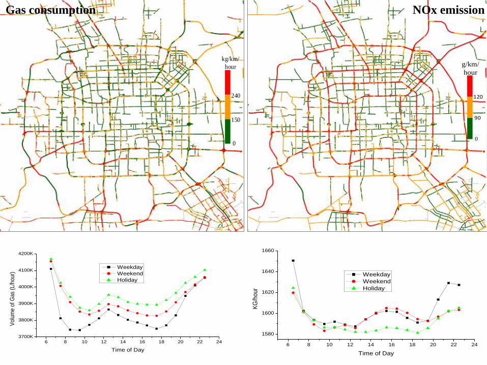
6 8 10 12 14 16 18 20 22 24
3700K
3800K
3900K
4000K
4100K
4200K
Volu
me o
f G
as
(L/h
our)
Time of Day
Weekday
Weekend
Holiday
6 8 10 12 14 16 18 20 22 24
1580
1600
1620
1640
1660K
G/h
our
Time of Day
Weekday
Weekend
Holiday
Gas consumption NOx emission
0
150
240
kg/km/
hour
90
120
g/km/
hour
0
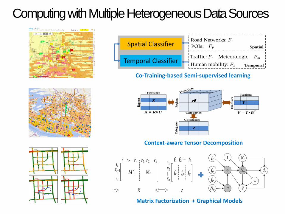
POIs: Spatial
Fh Temporal
Road Networks: Fr
Ft FmMeteorologic:Traffic:
Human mobility:
FpSpatial Classifier
Temporal Classifier
Co-Training-based Semi-supervised learning
Computing with Multiple Heterogeneous Data Sources
Context-aware Tensor Decomposition
Matrix Factorization + Graphical Models
Categories
Reg
ions
Categories
Cat
egor
ies
Reg
ions
Features
A
X = R×U
Z
Tim
e sl
ots
Regions
Y
Y = T×RT
X
fp
fg
t Nt
ɵ Na
v
dv
fr
w
Np α
g1 g2 g16ti
ti+1
tj
MG
g1 g2 g16 r1 r2 rnti
ti+1
tj
Mr
r1 r2 rn r1
r2
rn
f1 f2 fk
XY Z
M G fr fpM r fg
0
150
240
kg/km
3 –
4 PM
Gas
Con
sum
ptio
n
2013/09/17
Tuesday
2013/09/21
Saturday
2013/10/02
National Holiday
0
kg/km
12
30
CO
3 –
4 PM
Take Away Messages
• 3B: Big city, Big challenges, Big data
• 3M: Data Management, Mining and Machine learning
• 3W: Win-Win-Win: people, city, and the environment
3∙BMW