SANDIA REPORTSAND2007-5983Unlimited ReleasePrinted September 2007

LDRD Final Report:Robust Analysis of Large-scaleCombinatorial Applications

William E. Hart, Robert D. Carr, Cynthia A. Phillips, Jean-Paul Watson,Nicholas L. Benavides, Harvey Greenberg, and Todd Morrison

Prepared bySandia National LaboratoriesAlbuquerque, New Mexico 87185 and Livermore, California 94550

Sandia is a multiprogram laboratory operated by Sandia Corporation,a Lockheed Martin Company, for the United States Department of Energy’sNational Nuclear Security Administration under Contract DE-AC04-94-AL85000.

Approved for public release; further dissemination unlimited.

Issued by Sandia National Laboratories, operated for the United States Department of Energy by SandiaCorporation.

NOTICE: This report was prepared as an account of work sponsored by an agency of the United StatesGovernment. Neither the United States Government, nor any agency thereof, nor any of their employees,nor any of their contractors, subcontractors, or their employees, make any warranty, express or implied,or assume any legal liability or responsibility for the accuracy, completeness, or usefulness of any infor-mation, apparatus, product, or process disclosed, or represent that its use would not infringe privatelyowned rights. Reference herein to any specific commercial product, process, or service by trade name,trademark, manufacturer, or otherwise, does not necessarily constitute or imply its endorsement, recom-mendation, or favoring by the United States Government, any agency thereof, or any of their contractorsor subcontractors. The views and opinions expressed herein do not necessarily state or reflect those ofthe United States Government, any agency thereof, or any of their contractors.

Printed in the United States of America. This report has been reproduced directly from the best availablecopy.

Available to DOE and DOE contractors fromU.S. Department of EnergyOffice of Scientific and Technical InformationP.O. Box 62Oak Ridge, TN 37831

Telephone: (865) 576-8401Facsimile: (865) 576-5728E-Mail: reports@adonis.osti.govOnline ordering: http://www.osti.gov/bridge

Available to the public fromU.S. Department of CommerceNational Technical Information Service5285 Port Royal RdSpringfield, VA 22161

Telephone: (800) 553-6847Facsimile: (703) 605-6900E-Mail: orders@ntis.fedworld.govOnline ordering: http://www.ntis.gov/help/ordermethods.asp?loc=7-4-0#online

DEP

ARTMENT OF ENERGY

• • UN

ITED

STATES OF AM

ERI C

A

2

SAND2007-5983Unlimited Release

Printed September 2007

LDRD Final Report:Robust Analysis of Large-scale Combinatorial

Applications

William E. Hart, Robert D. Carr, Cynthia A. Phillips, and Jean-Paul WatsonDiscrete Math and Complex Systems Department

Sandia National LaboratoriesP.O. Box 4800

Albuquerque, NM 87185-1318

Nicolas L. BenavidesSanta Clara University500 El Camino Real

Santa Clara, CA 95053

Harvey Greenberg and Todd MorrisonDepartment of Mathematics

University of Colorado, Denver1200 Larimer St.

Denver, CO 80204

Abstract

Discrete models of large, complex systems like national infrastructures andcomplex logistics frameworks naturally incorporate many modeling uncertain-ties. Consequently, there is a clear need for optimization techniques that canrobustly account for risks associated with modeling uncertainties. This reportsummarizes the progress of the Late-Start LDRD “Robust Analysis of Large-scale Combinatorial Applications”. This project developed new heuristics forsolving robust optimization models, and developed new robust optimizationmodels for describing uncertainty scenarios.

3

Acknowledgments

We thank Regan Murray for collaborating on the application of robust optimization tech-niques to water security applications.

4

Contents1 Executive Summary . . . . . . . . . . . . . . . . . . . . . . . . . . . . . . . . . . . . . . . . . . . . . . . . . . . . . . . 92 Robust Optimization with CVaR . . . . . . . . . . . . . . . . . . . . . . . . . . . . . . . . . . . . . . . . . . . . 11

2.1 A CVaR Integer Programming Formulation . . . . . . . . . . . . . . . . . . . . . . . . . 112.2 Preliminary Computational Results . . . . . . . . . . . . . . . . . . . . . . . . . . . . . . . . 142.3 Minimizing CVaR . . . . . . . . . . . . . . . . . . . . . . . . . . . . . . . . . . . . . . . . . . . . . 15

3 A New Formulation for Minimizing Regret . . . . . . . . . . . . . . . . . . . . . . . . . . . . . . . . . . 193.1 A Minimax Regret Formulation . . . . . . . . . . . . . . . . . . . . . . . . . . . . . . . . . . . 193.2 A New Minimax Regret Formulation . . . . . . . . . . . . . . . . . . . . . . . . . . . . . . 213.3 Facility Location and Sensor Placement . . . . . . . . . . . . . . . . . . . . . . . . . . . . 24

4 Enabling Technologies . . . . . . . . . . . . . . . . . . . . . . . . . . . . . . . . . . . . . . . . . . . . . . . . . . . . . 254.1 The Pyomo Modeling Tool . . . . . . . . . . . . . . . . . . . . . . . . . . . . . . . . . . . . . . 254.2 Goal Programming in PICO . . . . . . . . . . . . . . . . . . . . . . . . . . . . . . . . . . . . . . 26

References . . . . . . . . . . . . . . . . . . . . . . . . . . . . . . . . . . . . . . . . . . . . . . . . . . . . . . . . . . . . . . . . . . . 28

AppendixA Robust Optimization Journal Article . . . . . . . . . . . . . . . . . . . . . . . . . . . . . . . . . . . . . . . . 29B Pyomo Technical Report . . . . . . . . . . . . . . . . . . . . . . . . . . . . . . . . . . . . . . . . . . . . . . . . . . . 30

5

Figures1 Data points generated showing trade-offs between CVaR and the expected

performance. . . . . . . . . . . . . . . . . . . . . . . . . . . . . . . . . . . . . . . . . . . . . . . . . . 18

6

Tables1 Results for minimizing expected performance with increasingly tight bounds

on CVaR. Runs are limited to 3600 seconds, Gap = Incumbent−Best BoundIncumbent . . . 15

2 Results for minimizing expected performance with increasingly tight boundson CVaR. Runs are limited to 1800 seconds, Gap = Incumbent−Best Bound

Incumbent . . . 163 Results for minimizing weighted sum formulation with bounds on CVaR. . . 174 Results for minimizing CVaR with heuristic solvers. . . . . . . . . . . . . . . . . . . 185 Runtime results in seconds for computing an LP bound on CVaR. . . . . . . . . 18

7

8

1 Executive Summary

Many real-world problems are concerned with maximizing or minimizing an objective (e.g.maximizing profit, minimizing costs, or lowering of risk). Optimization methods are com-monly used for these applications to find a best possible solution to a problem mathe-matically, which improves or optimizes the performance of the system. Many real-worldoptimization problems involve discrete decisions, such as selecting investments, allocatingresources and scheduling activities. These discrete optimization problems arise in manyapplication areas like infrastructure surety, military inventory and transportation logistics,production planning and scheduling, and informatics.

Discrete models of large, complex systems like national infrastructures and complexlogistics frameworks naturally incorporate many modeling uncertainties. Model factorslike transportation times and demands in water networks are inherently variable. Further,other information like logistical costs and infrastructure capacity limitations may only beknown at a coarse, aggregate level of precision. Although such models can be optimizedusing average or estimated data, solutions found in this manner often fail to reflect the risksassociated with these modeling uncertainties.

Consequently, there is a clear need for discrete optimization methods that can robustlyaccount for risks associated with modeling uncertainties. So called robust optimizationtechniques find solutions that optimize a performance objective while accounting for thesemodeling uncertainties. Sandia’s discrete optimization group has developed robust opti-mization methods for a variety of real-world problems, but a consistent challenge has beenthat existing robust optimization approaches cannot be reliably used on large-scale appli-cations.

This report summarizes the progress of the Late-Start LDRD “Robust Analysis ofLarge-scale Combinatorial Applications”. This project’s accomplishments can be groupedinto three areas:

• Robust Optimization with CVaR: Conditional value-at-risk (CVaR) is a risk met-ric that is commonly used in financial models. Discrete optimization formulationsof CVaR have recently been developed for water security and facility location ap-plications, but only small-scale problems can be practically solved with existing op-timization solvers. We describe experimental analyses of CVaR problems that (a)characterize computational bottlenecks and (b) evaluate the performance of heuristicoptimization solvers.

• Minimizing Regret: The regret of a decision made under uncertainty refers to theimpact of not having made an optimal decision without uncertainties. Uncertaintyin discrete optimization models can often be analyzed by minimizing the maximumregret. We present a new minimax regret formulation that is mathematically strongerthan previous approaches.

9

• Enabling Technologies: Several software development efforts were initiated to en-able the solution of robust optimization applications. A new search strategy forthe PICO integer programming solver was developed to avoid over-constraining thesearch in risk-constrained applications. Further, a Python module was developed toflexibly model and solve the nonlinear formulations that commonly arise in discreteoptimization problems.

We expect these new capabilities to directly impact Sandia’s ability to address modelinguncertainties in a variety of new and ongoing efforts. For example, the following projectswill leverage these capabilities in FY08:

• Water Security (EPA): The EPA has been funding Sandia to develop contaminantwarning systems for water distribution systems. A key element of this is the place-ment of sensors, which involves uncertain data. The EPA is interested in Sandia’srobust optimization capabilities, and the new formulation developed in this LDRDaddresses a key scalability challenge in this work: accounting for seasonal demandvaritions. We do not expect this model to be used within the current SNL-EPA WFOproject, but in FY08 we will leverage this when formulating a new WFO project withthe EPA.

• Scheduling Investments in Future Energy Supplies (LDRD): An ongoing LDRDproject will leverage these robust optimization capabilities to address uncertaintiesin models used to plan investments our nation’s energy infrastructure. Addressinguncertainties is a fundamental aspect of these models, but robust optimization is notthe technical focus. However, our robust optimization results can be immediatelyapplied to these models.

• Aircraft Fleet Planning (LMSV): An ongoing Shared Vision project with LockheedMartin will leverage the Pyomo software developed in this project to support a newapplication initiative. This software will be used to formulate and solve an aircraftfleet planning logistics model. In particular, Pyomo’s ability to interface with aircraftdesign sub-models is critical to this project. Further, there is significant uncertaintyin these logistics problems, and thus robust optimization techniques are particularlyvaluable for these planning activities.

10

2 Robust Optimization with CVaR

The conditional value-at-risk (CVaR) metric is a risk measure that has been widely used inthe finance community. The CVaR risk measure can be applied to applications in whichproblem uncertainty can be characterized by a set of scenarios. For example, in infrastruc-ture security applications, scenarios might consider possible failures of infrastructure com-ponents due to attacks. In logistics models, scenarios might characterize the time neededto transport materials.

These types of scenario-based optimization formulations are very flexible. They canintegrate complex uncertainty models. For example, they allow optimization methods tobe used effectively with data generated by more detailed simulation models. Further, theyallow for the characterization of the impacts of uncertainties in a generic manner.

For example, we have recently used CVaR to model risk in a water security applica-tions [13]. The goal of this model was to place sensors so as to minimize the expectedimpact of a contamination event (see model (SP) below). In this application, contamina-tion impacts are considered for a variety of scenarios that are defined by the time, locationand contaminant characteristics of possible contamination events. A variety of contamina-tion impact metrics have been developed, such as minimizing population consumption ofcontaminated water and minimizing time to detection. Evaluation of a scenario’s impactinvolves a hydraulic simulation in a water distribution system, including a simulation ofcontaminant transport in the network.

In this section we describe an integer programming (IP) model for CVaR for sensorplacement. Preliminary computational results highlight challenges with solving this IP onreal-world sensor placement applications. We address this challenge in several ways. First,we consider bottlenecks in the solution of the CVaR integer program (IP); specifically, weconsider the runtime of the root linear programming relaxation. Although the cost of thisrelaxation can be reduced, the total cost of the CVaR IP remains large. Consequently, weconsider the application of several IP heuristics.

2.1 A CVaR Integer Programming Formulation

Value-at-Risk (VaR) is a percentile-based metric usually defined as the maximal allowableloss within a certain confidence level γ ∈ (0,1) [12]. Mathematically, suppose we havea function, f (~x,ξ ), where ~x is a vector of decision variables and ξ is a vector of randomvariables. Then f (~x,ξ ) is also a random variable, and we define:

VaR(~x,γ) = minu : Pr[ f (x,ξ )≤ u]≥ γ.For example, suppose f (~x,ξ ) = ξ and Pr(ξ = 10) = Pr(ξ = 100) = 1

2 . Then,

VaR(x,γ) =

10 if 0≤ γ < .5100 if .5≤ γ < 1.

11

If we think of f as some measure of risk, the chance constraint is a confidence level(γ) that the risk not exceed some level, which we minimize. (We can equivalently writePr[ f (~x,ξ ) > u] ≤ 1− γ , which says that we want the probability of exceeding some level(u) to be less than 1− γ , say 5%. The objective is to minimize that level subject to thatchance constraint.) We generally want to know what the VaR is at various values of γ ,ranging from 90% to 99%.

The Conditional Value-at-Risk (CVaR) is a related metric which measures the condi-tional expectation of losses exceeding VaR at a given confidence level. Technically, thisexpectation is the Tail Conditional Expectation (TCE),

TCE(~x,γ) = E[

f (~x,ξ )∣∣ f (~x,ξ )≥ VaR(~x,γ)

],

and CVaR is linearization of TCE investigated by Uryasev and Rockafellar [11]. CVaRapproximates TCE with a continuous, piecewise-linear function of γ .

To see this relation, let Ω be the set of scenarios, let ωi the probability of realizingscenario i, and fi(~x) be the value of f in scenario i ∈ Ω. Observe that by defining anindicator variable, ρi, to be 1 if fi ≥ VaR and 0 otherwise, we can write TCE as,

TCE(x,γ) = ∑i fiωiρi

∑i ωiρi.

Next we define a vector of auxiliary variables y = (yi) such that

yi = max0, fi−VaR.

Then we can write,

TCE(x,γ) = ∑i fiωiρi

∑i ωiρi= VaR+ ∑i( fi−VaR)ωiρi

∑i ωiρi= VaR+ ∑i ωiyi

∑i ωiρi.

Noting that ∑i ωiρi ≈ γ , we define CVaR as the approximation,

CVaR(x,γ) = VaR+1γ ∑

iωiyi.

Then, since γ ≤ ∑i ωiρi, we have,

TCE(x,γ) = VaR+ ∑i ωiyi

∑i ωiρi≤ VaR+

1γ ∑

iωiyi = CVaR(x,γ).

Graphically, CVaR holds with equality at those points where γ = ∑i ωiρi (the points wherethe usual function steps) and joins the steps with a linear overestimate of CVaR. Thus,CVaR serves as an approximation of the bilinear form found in the formulation of TCE andis continuous in γ .

12

We illustrate the use of CVaR by developing an IP for minimizing the CVaR of impactsin sensor placement problem. We consider the sensor placement formulation describedBerry et al. [6]:

(SP) min ∑a∈A

αa ∑i∈La

daixai (1)

∑i∈La

xai = 1 ∀a ∈A (2)

xai ≤ si ∀a ∈A , i ∈La (3)

∑i∈L

si ≤ p (4)

si ∈ 0,1 ∀i ∈ L (5)0≤ xai ≤ 1 ∀a ∈A , i ∈La (6)

This IP minimizes the expected impact of a set of contamination scenarios defined by A .For each scenario a, La ⊆ L defines the set of locations that can be contaminated in thescenario, αa defines the weight of the scenario, and dai defines the impact of the contam-ination; Berry et al. [6] consider a water security application, where typical impacts arepopulation exposure, extent of contamination, and time to detection. The si variables indi-cate where sensors are placed in the network, subject to a budget p, and the xia variablesindicate whether scenario a is witness at location i by a sensor.

A limitation of this model is that is considers only the weighted average of scenarioimpacts, the expected impact. Thus rare, but potentially catastrophic, contamination sce-narios will be essentially ignored. To address these possibly disastrous extremes we needto include some measure of the risk associated with a particular solution. As a risk metricthat is sensitive to large tails CVaR is well suited to this task. Hence we have formulatedthe sensor placement problem with restricted risk:

(rrSP) min ∑a∈A

αa ∑i∈La

daixai (7)

∑i∈La

xai = 1 ∀a ∈A (8)

xai ≤ si ∀a ∈A , i ∈La (9)

∑i∈L

si ≤ p (10)

si ∈ 0,1 ∀i ∈ L (11)0≤ xai ≤ 1 ∀a ∈A , i ∈La (12)

v+1γ ∑

a∈A

αaya ≤maxCVaR (13)

ya ≥ ∑i∈La

daixai− v ∀a ∈A (14)

ya ≥ 0 ∀a ∈A (15)

Alternately, we can formulate the risk adverse sensor placement problem as a goal program-ming problem by dropping the maximum CVaR constraint (13) and replacing the objective

13

function (7) with,

(raSP) min ∑a∈A

αa ∑i∈La

daixai +λ

(v+

1γ ∑

a∈A

αaya

).

Either formulation allows us to explore the efficient frontier of trade-offs between min-imizing the expected case versus reducing our exposure to risky outliers. In the first formu-lation this can be done by solving the problem for a number of values, maxCVaR, assumingwe know a reasonable range to work in. The second formulation avoids the need to knowthis range, instead we explore the efficient frontier by varying the parameter λ . Computa-tional issues and the difficulties inherent in exploring the efficient frontier of non-convex,multiple-objective problems (such as integer programs) will probably require the use ofboth formulations or a combination of the two.

2.2 Preliminary Computational Results

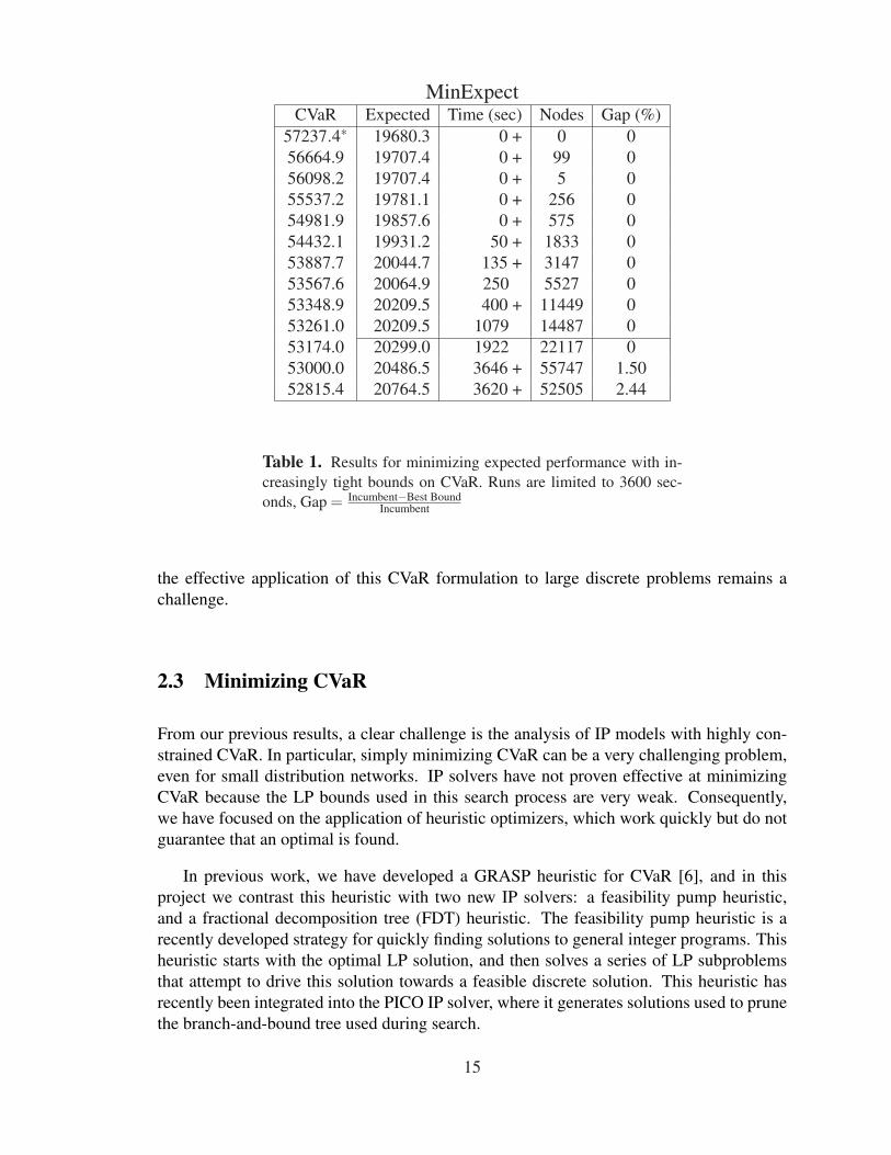
Our preliminary computational analysis of CVaR considers a small sensor placement ap-plication for water security for which we can solve many CVaR optimization problems tooptimality. We explore the efficient frontier by solving for the minimum expected valuesubject to an upper bound (“maxCVaR”) on CVaR. Since we would like to investigate onlythe non-trivial points we seed our search by solving a weighted sum formulation (“Min-Both”) with a very small weight (λ = .01) on CVaR. Table 1 shows results from solving asequence of problems with an increasingly tighter bound (99% of the previous bound).

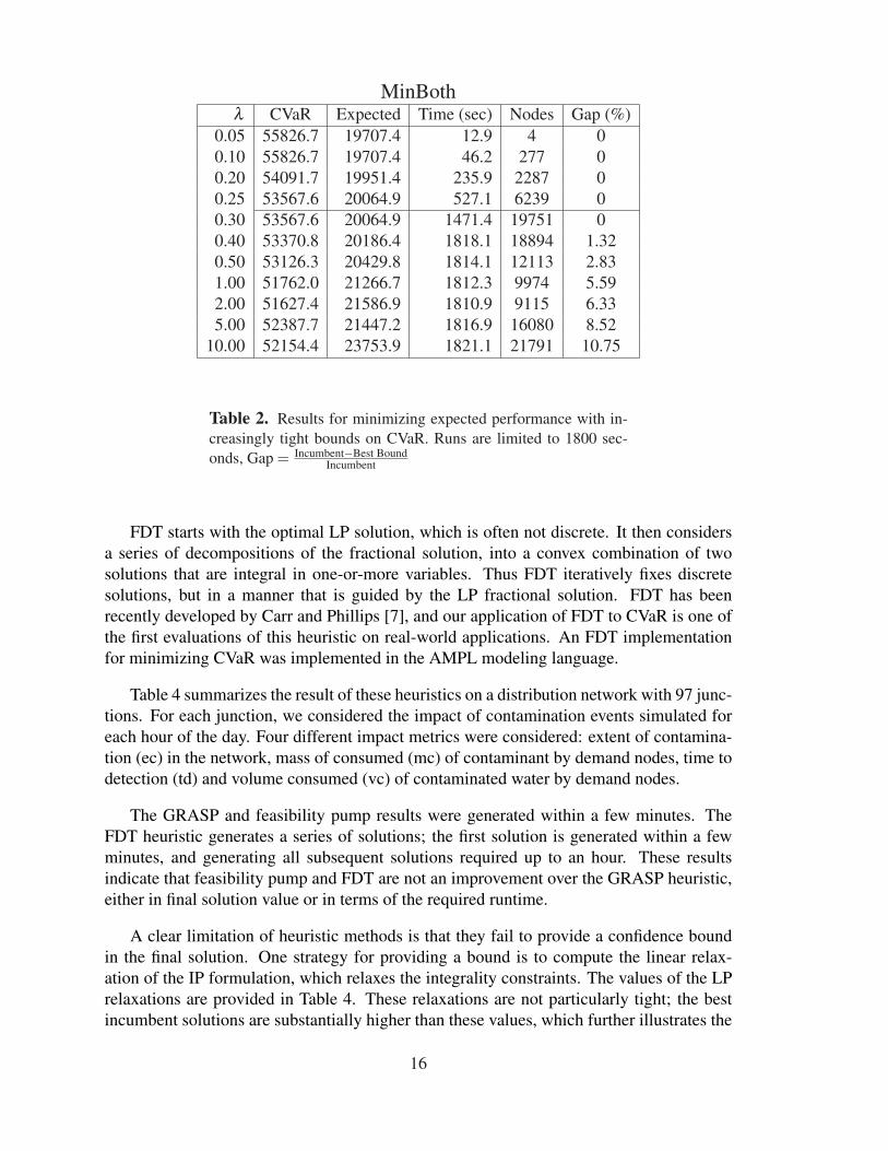
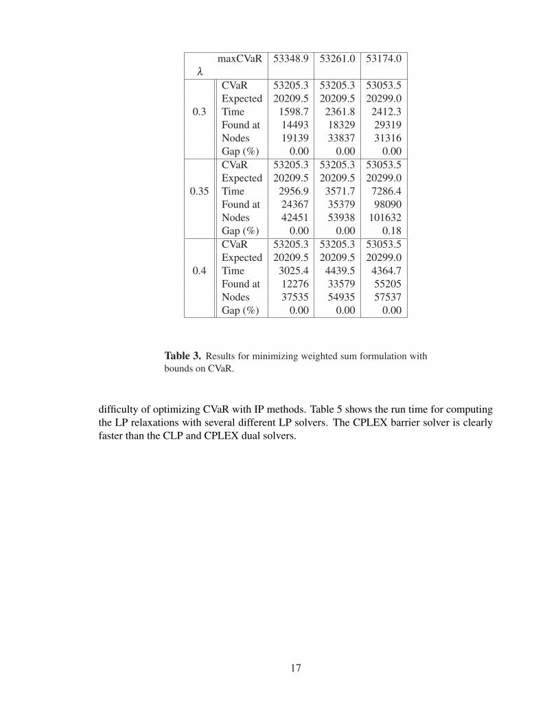
Table 2 shows results from solving for the minimum of a weighted sum, expected im-pact plus λ ×CVaR. In these runs run time was limited to 30 minutes, note that for somehigher values of λ this was not sufficient to find even as good an incumbent as previousruns. Also, different values for λ may correspond to the same frontier point, yet requirevastly different computational effort. Further, Table 3 shows a combination approach wherewe solve the weighted sum formulation subject to CVaR bound. These runs clearly showthat the efficient frontier is stair-stepped with some points on the frontier weakly domi-nated.

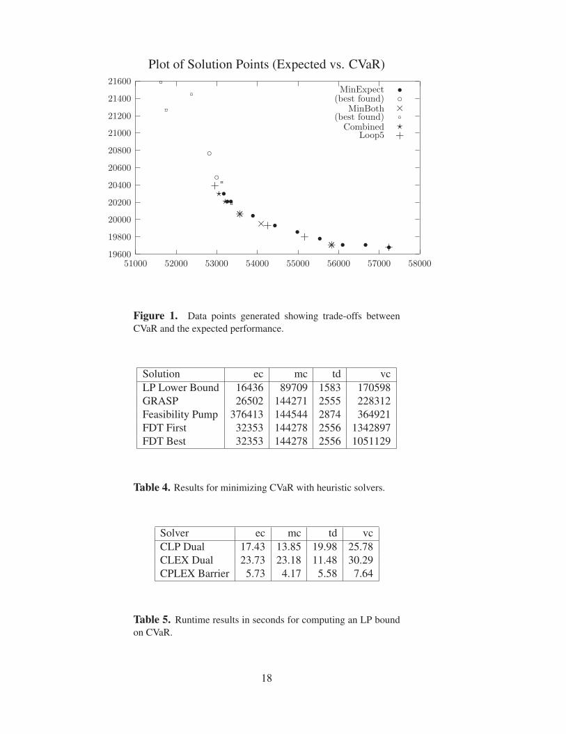
The data points from these experiments are plotted in Figure 1, which illustrates theextent of the frontier that we have searched. Points in the lower right-hand side of thisfrontier are easy to find, while points on the upper left-hand side are much more difficult.

Appendix A includes an article submitted for publication to the Journal of InfrastructureSystems. This article summarizes the use of this CVaR IP for real-world sensor placementapplications; Watson, Hart and Murray [13] describes a preliminary version of this article,and a journal submission was completed as part of this LDRD. This article shows thedifficulty associated with optimizing large-scale CVaR models. We were not able to solvethe IP formulation for real-world sensor placement applications. Further, it was difficultto assess whether heuristic optimization methods provided near-optimal solutions. Thus,

14

MinExpectCVaR Expected Time (sec) Nodes Gap (%)

57237.4∗ 19680.3 0 + 0 056664.9 19707.4 0 + 99 056098.2 19707.4 0 + 5 055537.2 19781.1 0 + 256 054981.9 19857.6 0 + 575 054432.1 19931.2 50 + 1833 053887.7 20044.7 135 + 3147 053567.6 20064.9 250 5527 053348.9 20209.5 400 + 11449 053261.0 20209.5 1079 14487 053174.0 20299.0 1922 22117 053000.0 20486.5 3646 + 55747 1.5052815.4 20764.5 3620 + 52505 2.44

Table 1. Results for minimizing expected performance with in-creasingly tight bounds on CVaR. Runs are limited to 3600 sec-onds, Gap = Incumbent−Best Bound

Incumbent

the effective application of this CVaR formulation to large discrete problems remains achallenge.

2.3 Minimizing CVaR

From our previous results, a clear challenge is the analysis of IP models with highly con-strained CVaR. In particular, simply minimizing CVaR can be a very challenging problem,even for small distribution networks. IP solvers have not proven effective at minimizingCVaR because the LP bounds used in this search process are very weak. Consequently,we have focused on the application of heuristic optimizers, which work quickly but do notguarantee that an optimal is found.

In previous work, we have developed a GRASP heuristic for CVaR [6], and in thisproject we contrast this heuristic with two new IP solvers: a feasibility pump heuristic,and a fractional decomposition tree (FDT) heuristic. The feasibility pump heuristic is arecently developed strategy for quickly finding solutions to general integer programs. Thisheuristic starts with the optimal LP solution, and then solves a series of LP subproblemsthat attempt to drive this solution towards a feasible discrete solution. This heuristic hasrecently been integrated into the PICO IP solver, where it generates solutions used to prunethe branch-and-bound tree used during search.

15

MinBothλ CVaR Expected Time (sec) Nodes Gap (%)

0.05 55826.7 19707.4 12.9 4 00.10 55826.7 19707.4 46.2 277 00.20 54091.7 19951.4 235.9 2287 00.25 53567.6 20064.9 527.1 6239 00.30 53567.6 20064.9 1471.4 19751 00.40 53370.8 20186.4 1818.1 18894 1.320.50 53126.3 20429.8 1814.1 12113 2.831.00 51762.0 21266.7 1812.3 9974 5.592.00 51627.4 21586.9 1810.9 9115 6.335.00 52387.7 21447.2 1816.9 16080 8.52

10.00 52154.4 23753.9 1821.1 21791 10.75

Table 2. Results for minimizing expected performance with in-creasingly tight bounds on CVaR. Runs are limited to 1800 sec-onds, Gap = Incumbent−Best Bound

Incumbent

FDT starts with the optimal LP solution, which is often not discrete. It then considersa series of decompositions of the fractional solution, into a convex combination of twosolutions that are integral in one-or-more variables. Thus FDT iteratively fixes discretesolutions, but in a manner that is guided by the LP fractional solution. FDT has beenrecently developed by Carr and Phillips [7], and our application of FDT to CVaR is one ofthe first evaluations of this heuristic on real-world applications. An FDT implementationfor minimizing CVaR was implemented in the AMPL modeling language.

Table 4 summarizes the result of these heuristics on a distribution network with 97 junc-tions. For each junction, we considered the impact of contamination events simulated foreach hour of the day. Four different impact metrics were considered: extent of contamina-tion (ec) in the network, mass of consumed (mc) of contaminant by demand nodes, time todetection (td) and volume consumed (vc) of contaminated water by demand nodes.

The GRASP and feasibility pump results were generated within a few minutes. TheFDT heuristic generates a series of solutions; the first solution is generated within a fewminutes, and generating all subsequent solutions required up to an hour. These resultsindicate that feasibility pump and FDT are not an improvement over the GRASP heuristic,either in final solution value or in terms of the required runtime.

A clear limitation of heuristic methods is that they fail to provide a confidence boundin the final solution. One strategy for providing a bound is to compute the linear relax-ation of the IP formulation, which relaxes the integrality constraints. The values of the LPrelaxations are provided in Table 4. These relaxations are not particularly tight; the bestincumbent solutions are substantially higher than these values, which further illustrates the

16

maxCVaR 53348.9 53261.0 53174.0λ

CVaR 53205.3 53205.3 53053.5Expected 20209.5 20209.5 20299.0

0.3 Time 1598.7 2361.8 2412.3Found at 14493 18329 29319Nodes 19139 33837 31316Gap (%) 0.00 0.00 0.00CVaR 53205.3 53205.3 53053.5Expected 20209.5 20209.5 20299.0

0.35 Time 2956.9 3571.7 7286.4Found at 24367 35379 98090Nodes 42451 53938 101632Gap (%) 0.00 0.00 0.18CVaR 53205.3 53205.3 53053.5Expected 20209.5 20209.5 20299.0

0.4 Time 3025.4 4439.5 4364.7Found at 12276 33579 55205Nodes 37535 54935 57537Gap (%) 0.00 0.00 0.00

Table 3. Results for minimizing weighted sum formulation withbounds on CVaR.

difficulty of optimizing CVaR with IP methods. Table 5 shows the run time for computingthe LP relaxations with several different LP solvers. The CPLEX barrier solver is clearlyfaster than the CLP and CPLEX dual solvers.

17

Plot of Solution Points (Expected vs. CVaR)

19600

19800

20000

20200

20400

20600

20800

21000

21200

21400

21600

51000 52000 53000 54000 55000 56000 57000 58000

MinExpect

sssssss

sss

s(best found)

c

c

cMinBoth

×××

××

×(best found)

Combined

??

?Loop5

+++

++

+

+

Figure 1. Data points generated showing trade-offs betweenCVaR and the expected performance.

Solution ec mc td vcLP Lower Bound 16436 89709 1583 170598GRASP 26502 144271 2555 228312Feasibility Pump 376413 144544 2874 364921FDT First 32353 144278 2556 1342897FDT Best 32353 144278 2556 1051129

Table 4. Results for minimizing CVaR with heuristic solvers.

Solver ec mc td vcCLP Dual 17.43 13.85 19.98 25.78CLEX Dual 23.73 23.18 11.48 30.29CPLEX Barrier 5.73 4.17 5.58 7.64

Table 5. Runtime results in seconds for computing an LP boundon CVaR.

18

3 A New Formulation for Minimizing Regret

The regret of a decision made under uncertainty refers to the impact of not having madean optimal decision without uncertainties. For example, consider the context of selectinga facility location to meet “customer” demand (e.g. locating a fire station or waste dump).Facility demands are uncertain, and these uncertainties can often be characterized as aset of potential demand scenarios. In practice, one or more of these scenarios is likely todominate future usage of the facility, but further information is unavailable when a decisionmaker selects the facility location.

A minimax regret formulation minimizes the regret of a decision across all scenarios.Here, regret can be characterized as the difference between a solution and the solution valueoptimized for a particular scenario:

fi(x)− f ∗iso the canonical minimax formulation is

minxmaxi fi(x)− f ∗i .

This is also called the worst-case regret, since we are minimizing the worst regret overall.

Chen et al. [8] consider a minimax regret model that minimizes the worst regret overthe best 100α% (say 95%) of the scenarios. This is better than minimizing the worst caseregret when one does not want an answer that is dominated by few scenarios (which mayoccur with low probability). For example, airports should not cater only to Thanksgivingand Christmas travel, but a worst-case regret formulation could do just that.

The following sections critique this model and present an alternative formulation thatcan be used to optimize this modified regret formulation. In particular, this reformulation ismotivated by the fact that the technique described by Chen et al. [8] is not practical for largefacility location applications. The final section below discusses the relationship betweenthis facility location model and the water security application discussed above.

3.1 A Minimax Regret Formulation

The original idea behind the facility location problem is that there is a network of customernode locations with a demand at each node and potential sites for p facilities that servicethese demands at a cost that increases with the distance from the facility to the customer.The problem then is to place the facilities so that the total demand is met at minimum cost.

We start with demand nodes i numbered from 1 to m so that the first n nodes (from 1to n) are the potential sites to place a facility, of which p of these sites will be chosen forputting facilities. We are given scenarios 1 to K. For scenario k we specify a demand hik foreach customer i and distance di jk between each customer i and potential facility location j.We assign a probability qk that scenario k will occur and the minimum cost Vk for satisfying

19

the total demand given one knows a head of time that scenario k will occur; Vk is obtainedby solving a facility location problem for scenario k alone.

The robust model proposed by Chen et al. [8] finds set of facility locations that minimizea regret measure. So, if x j for j = 1..n are binary variables that indicate where we will putour facilities and yi, j,k are binary variables that are 1 when customer i gets serviced byfacility j under scenario k, the total cost of meeting the demand for scenario k is

m

∑i=1

n

∑j=1

hikdi jkyi jk.

Since the lowest possible cost would be Vk, there is a regret of Rk from scenario k given by

Rk =m

∑i=1

n

∑j=1

hikdi jkyi jk−Vk.

We could minimize a weighted sum of regrets or a worst-case regret, but in both cases out-lier scenarios can significantly skew our solution. A worst-case regret may only be relevantfor a small number of extreme scenarios, and a weighted sum can be similarly skewed bylarge outlier values. Although we would want a solution to work well in principle for allscenarios, that fact that we have uncertainties in the relevance of these scenarios motivatesthe decision maker to ignore these extreme scenarios for the analysis.

Our robust measure based on regrets is to minimize the worst regret in the best 95% ofthe outcomes. If we have a binary variable zk indicating whether scenario k is in the best100α% of the regrets, then we will minimize the maximum regret W where for each k wehave the constraint

W +Rk(1− zk)≥ Rk,

which makes W larger than any regret Rk in the best 100α% (that is for which zk = 1).Notice that these constraints are designed to say nothing we didn’t already know when k isnot one of the selected scenarios (zk = 0), but say exactly what we want when k is a selectedscenario. To ensure that the z variables are set correctly, we need the constraint

K

∑k=1

qkzk ≥ α .

Unfortunately, the constraints that give lower bounds for W are non-linear, so we cannotsolve this formulation with an integer programming solver in a standard manner. Chen etal. [8] resolve this by guessing the constants mk to be as close to but bigger than the actualregrets Rk as possible. Then, the constraints

W +mk(1− zk)≥ Rk

can be used to bound W . The problem with this approach is that if these guesses for mk areoff, one may have to make new guesses and solve the IP all over again.

20

Finally, we have the normal facility location constraints for the x variables (indicatingfacilities) and the y variables (indicating which facility services each customer). Since weare placing p facilities, we have

n

∑j=1

x j = p.

Since in each scenario k, only one facility services any customer i, we have

n

∑j=1

yi jk = 1 ∀i ∈ 1, ..,m∀k ∈ 1, ..,K.

Since a facility cannot service a customer if it were never built, we have

yi jk ≤ x j ∀ j ∈ 1, ..,n∀i ∈ 1, ..,m∀k ∈ 1, ..,K.

As was stated earlier, our objective is to minimize W subject to the constraints of thissection.

3.2 A New Minimax Regret Formulation

We have come up with several ideas for improving the formulation discussed in the previoussection. The first idea is to turn the variable W into a constant by guessing its value to besome W ∗. We will soon see that this makes the cost of a single scenario easier to model as alinear function, and besides we had to make guesses in the previous IP as well. In keepingwith our robust modeling ideas, we should be able to model a truncated cost of a scenariok that is its actual cost if zk = 1, but only W ∗+ Vk if k were an outlier (zk = 0). Then, thecost of scenario k can be given by an almost linear function

(W ∗+Vk)(1− zk)+(Rk +Vk)zk. (16)

The only non-linearity is the product Rkzk, but we will explain later that this product can beclosely approximated by linear variables Fk, turning the single scenrio cost into the linearfunction

(W ∗+Vk)(1− zk)+Fk +Vkzk.

Going back to equation (16), notice that the cost is a convex combination of the truncatedcost W ∗+Vk and the actual cost Rk +Vk, with convex multipliers 1− zk and zk respectively.Then, zk takes on a value of either 0 or 1, depending on which of the actual and truncatedcosts were smaller since we wish to minimize cost.

We show the basic modeling idea behind the variables Fk that are used to determine Fk,and are the product of the cost (optimum single scenario plus regret) times zk.

Fk = (m

∑i=1

n

∑j=1

hikdi jkyi jk)zk.

21

Now, we can impose constraints that bound the variables Fk:

Fk = Fk +Vkzk,Vkzk ≤ Fk ≤ (W ∗+Vk)zk.

These constraints ensure that if the cost exceeds the threshold, that is

Fk/zk :=m

∑i=1

n

∑j=1

hikdi jkyi jk > W ∗+Vk,

then zk and Fk would be set to 0, which one can afford to do up to 1−α of the time, so thatFk would not exceed (W ∗+Vk)zk.

Our next idea is to define scaled versions of the LP relaxation for the facility locationformulation so that we could effectively model Fk and Fk, the versions of the cost and regretof the solution scaled by zk, for each scenario k. To achieve this, we create variables t jk andvi jk that we wish to satisfy

vi jk := yi jkzkt jk := x jzk.

The usual LP relaxation for facility location is

∑nj=1 x j = p 0≤ x≤ 1

∑nj=1 yi j = 1 ∀i ∈ 1, ..,m, y≥ 0

yi j ≤ x j ∀i ∈ 1, ..,m∀ j ∈ 1, ..,n,cost = ∑m

i=1 ∑nj=1 hidi jyi j.

(17)

Our constraints to scale this LP by zk are:

∑nj=1 t jk = pzk 0≤ t jk ≤ zk∀ j ∈ 1, ..,n,

∑nj=1 vi jk = zk ∀i ∈ 1, ..,m, v≥ 0

vi jk ≤ t jk ∀i ∈ 1, ..,m∀ j ∈ 1, ..,n,Fk = ∑m

i=1 ∑nj=1 hikdi jkvi jk.

(18)

If we take the above formulation and divide each of t,v, and F by zk, we get the usual LPrelaxation for facility location, which means that these scaled models create no additionalerror compared with the LP relaxation other than that from relaxing the binary variables ofthe problem.

Our third idea is to enforce t to be zk multiplied by the same x vector for all k whileallowing v to be zk multiplied by a different yi jk vector for each scenario k. This makessense since we want to make a placement of facilities that does not depend on scenariowhile which facility services a customer could depend on the scenario. In fact, we do notuse a k subscript for the x variables, but do use such a subscript for the y variables. Thismodeling distinction leads us to form constraints analogous to the single constraint

K

∑k=1

qkzk ≥ α . (19)

22

We may now have a constraint for each j ∈ 1, ..,n stating:

K

∑k=1

qkt jk ≥ αx j. (20)

Also, we can form another constraint analogous to

0≤ t jk ≤ zk, (21)

based on the idea that x j− t jk = x j(1− zk), so we can multiply 0≤ x≤ 1 by 1− zk as wellas by zk. Hence, we get

0≤ x j− t jk ≤ 1− zk. (22)

These are similar to the constraints

0≤ yi jk− vi jk ≤ 1− zk, (23)

except that we take advantage of x not depending on the scenario k.

Our robust model in its entirety, except that the objective function is left out, is asfollows:

Fk = ∑mi=1 ∑n

j=1 hikdi jkvi jk ∀k ∈ [K]Vkzk ≤ Fk ≤ (W ∗+Vk)zk ∀k ∈ [K]

∑nj=1 x j = p 0≤ x≤ 1

∑nj=1 yi jk = 1 ∀i ∈ [m]∀k ∈ [K] y≥ 0

yi jk ≤ x j ∀i ∈ [m]∀ j ∈ [n]∀k ∈ [K]∑n

j=1 t jk = pzk 0≤ t jk ≤ zk∀ j ∈ [n]∀k ∈ [K]∑n

j=1 vi jk = zk ∀i ∈ [m]∀k ∈ [K] v≥ 0vi jk ≤ t jk ∀i ∈ [m]∀ j ∈ [n]∀k ∈ [K]

∑Kk=1 qkzk ≥ α

∑Kk=1 qkt jk ≥ αx j ∀ j ∈ [n]

0 ≤ x j− t jk ≤ 1− zk ∀ j ∈ [n]∀k ∈ [K]0 ≤ yi jk− vi jk ≤ 1− zk ∀i ∈ [m]∀ j ∈ [n]∀k ∈ [K]

x,y,z, t,v integer.

(24)

As for the objective function, we have choices. One idea is for this IP to simply be afeasibility problem with no objective function. Another idea is to add up the cost of eachscenario k truncated by W ∗+Vk, and minimize. Thus an objective function could be

minimizeK

∑k=1

((W ∗+Vk)(1− zk)+Fk).

One can see by examining this IP model when the z variables all have 0,1 values that itsLP relaxation is as tight as that of the facility location problem for each scenario when thisintegality condition is satisfied. This indicates that ours is a better LP relaxation than thatof the previous section. This also indicates that branching on the z variables is particularlyimportant when solving our robust IP with branch-and-bound.

23

3.3 Facility Location and Sensor Placement

The sensor placement model (SP) discussed in Section 2 is closely related to the standardp-median formulation used for facility location. There is some additional structure thatcan be exploited in (SP), but otherwise it uses the same set of constraints. However, theCVaR formulation and our minimax regret formulation address different aspect of modelinguncertainties in sensor placement applications.

The CVaR model was developed to characterize the risk associated with different con-tamination events. In general, we wish to optimize expected performance, while constrain-ing such risk to acceptable level. But when drawing a correspondence with facility location,the CVaR model considers only a single scenario; the different contamination events cor-respond to different demands on a facility.

To better understand this correspondence, consider the placement of sensors to protectagainst contamination events at different seasons of the year. Water usage patterns will bequite different between summer and winter, and thus contamination events could propagatein very different manners and have different consequences. However, for each season thereis a set of possible contamination events that need to be considered, for different locationsand times of day for contamination. Thus, the seasons correspond to the scenarios that wehave considered for facility location.

This generalization of the sensor placement problem addresses one of the key limita-tions of existing sensor placement formulations. There are a large number of possible sce-narios that account for different conditions in the network and different characteristics ofcontamination events. However, existing approaches lump all of the contamination eventsin these scenarios into one set of events. As we noted earlier, this could lead to sensorplacement designs that are skewed towards particular contamination events in particularscenarios.

24

4 Enabling Technologies

Two enabling technologies were developed as part of our research efforts to facilitate thesolution of robust optimization applications. A new modeling tool, Pyomo, was developedto provide a more flexible environment for modeling and solving complex formulationslike robust optimization problems. Also, we developed a new search strategy for the PICOinteger programming solver that can manage constraint violations in a flexible manner andcache nearly feasible solutions.

4.1 The Pyomo Modeling Tool

Appendix B includes a technical report that describes the Python Optimization ModelingObjects (Pyomo) package. Pyomo is a Python package that can be used to define ab-stract problems, create concrete problem instances, and solve these instances with standardsolvers. Pyomo provides a capability that is commonly associated with algebraic modelinglanguages like AMPL and GAMS. However, Pyomo can leverage Python’s programmingenvironment to support the development of complex models and optimization solvers inthe same modeling environment.

Algebraic Modeling Languages (AMLs) are high-level programming languages for de-scribing and solving mathematical problems, particularly optimization-related problems [10].AMLs like AIMMS [1], AMPL [2, 9] and GAMS [4] have programming languages with anintuitive mathematical syntax that supports concepts like sparse sets, indices, and algebraicexpressions. AMLs provide a mechanism for defining variables and generating constraintswith a concise mathematical representation, which is essential for real-world problems thatcan involve thousands of constraints and variables.

An alternative strategy for modeling mathematical problems is to use a standard pro-gramming language in conjunction with a software library that uses object-oriented de-sign to support similar mathematical concepts. Although these modeling libraries sac-rifice the intuitive mathematical syntax of an AML, they allow the user to leverage thegreater flexibility of standard programming languages. For example, modeling librarieslike FLOPC++ [3] and OPL [5] enable the solution of large, complex problems within auser-defined application.

Pyomo is a Python package that can be used to define abstract problems, create concreteproblem instances, and solve these instances with standard solvers. Like other modelinglibraries, Pyomo can generate problem instances and apply optimization solvers with afully expressive programming language. Further, Python is a noncommercial languagewith a very large user community, which will ensure robust support for this language on awide range of compute platforms.

Python is a powerful dynamic programming language that has a very clear, readablesyntax and intuitive object orientation. Python’s clean syntax allows Pyomo to express

25

mathematical concepts in a reasonably intuitive manner. Further, Pyomo can be used withinan interactive Python shell, thereby allowing a user to interactively interrogate Pyomo-based models. Thus, Pyomo has many of the advantages of both AML interfaces andmodeling libraries.

Pyomo was developed as part of this project to facilitate the development of heuristicoptimizers for complex applications like robust optimization problems. Specifically, ourgoal was to develop heuristics like FDT in Python using Pyomo’s modeling objects. Unfor-tunately, this goal was not realized due to time constraints; instead, we implemented FDTwith a rather awkward AMPL model. However, our prototype of Pyomo can be used tomodel and solve simple integer programming applications using Sandia’s PICO IP solver.We expect Pyomo to mature as we use it for applications, and that it will play a key rolein the development of new applications. In FY08, we plan to use Pyomo to analyze air-craft fleet planning applications under Lockheed Martin Shared Vision funding, includingrobust planning models. We currently plan to release Pyomo under an open-source licenseto encourage its use by external collaborators.

4.2 Goal Programming in PICO

In practice, satisfying a risk constraint exactly in a robust optimization formulation is lesscrucial than finding an effective compromise between the optimization objective and theperformance risk. Thus, a risk constraint is better described as a goal that we want tomeet, and risk-constrained robust optimization formulations can be effectively cast as goalprogramming models.

Solution of goal programming models for robust optimization differs from standard dis-crete optimization in at least two important ways. First, the outcome of robust optimizationis a set of solutions that represent trade-offs between the optimization objective and risk.Thus, the optimizer needs to maintain this set of solutions, and filter out solutions that aredominated by other solutions (i.e. they are not better in either the objective or risk valuethan at least one other solution). This is an example of a bi-criteria optimization problem,and standard sorting techniques can be used to maintain a set of undominated solutions.

Second, the search process needs to be adapted to explicitly recognize goals. Standarddiscrete optimization techniques do not allow the search to focus on infeasible solutions; infact, the efficiency of a discrete optimization solver is often related to how well it eliminatesinfeasible solutions. When considering goal constraints, we need to allow for infeasiblesolutions. This can be done by biasing search towards solutions that meet our goals. Thisis a natural extension of many heuristic solvers, which simply augment the objective witha penalty associated with how much the goal constraint is violated.

Support for goal constraints is being added to Sandia’s PICO integer programmingsolver. The heuristic solvers that PICO supports for integer programming formulationscan recognize goals and treat them appropriately, and PICO maintains a pool of solutions

26

that represent different trade-offs between the optimization objective and these goal values.This capability will be included in an forthcoming release of PICO (planned for fall of2007).

27

References

[1] AIMMS home page.

[2] AMPL home page.

[3] FLOPC++ home page.

[4] GAMS home page.

[5] OPL home page.

[6] J. BERRY, W. E. HART, C. E. PHILLIPS, J. G. UBER, AND J.-P. WATSON, Sensorplacement in municiple water networks with temporal integer programming models,J. Water Resources Planning and Management, 132 (2006), pp. 218–224.

[7] R. D. CARR AND C. A. PHILLIPS, Fractional decomposition trees: Finding feasiblesolutions to integer programs with bounded integrality gaps, Tech. Report SAND2006-7947, Sandia National Laboratories, 2007.

[8] G. CHEN, M. S. DASKIN, Z.-J. SHEN, AND S. URYASEV, The alpha-reliable mean-excess regret model for stochastic facility location modeling, Naval Research Logis-tics. (to appear).

[9] R. FOURER, D. M. GAY, AND B. W. KERNIGHAN, AMPL: A Modeling Languagefor Mathematical Programming, 2nd Ed., Brooks/Cole–Thomson Learning, PacificGrove, CA, 2003.

[10] J. KALLRATH, Modeling Languages in Mathematical Optimization, Kluwer Aca-demic Publishers, 2004.

[11] R. T. ROCKAFELLAR AND S. URYASEV, Conditional value-at-risk for general lossdistributions, Journal of Banking and Finance, 26 (2002), pp. 1443–1471.

[12] N. TOPALOGLOU, H. VLADIMIROU, AND S. ZENIOS, CVaR models with selectivehedging for international asset allocation, Journal of Banking and Finance, 26 (2002),pp. 1535–1561.

[13] J.-P. WATSON, W. E. HART, AND R. MURRAY, Formulation and optimization ofrobust sensor placement problems for contaminant warning systems, in Proc. WaterDistribution System Symposium, 2006.

A Robust Optimization Journal Article

29

Formulation and Optimization of Robust Sensor PlacementProblems for Drinking Water Contamination Warning

Systems

Jean-Paul Watson∗ Regan Murray† William E. Hart‡

Abstract

The sensor placement problem in contamination warning system design for water distri-

bution networks involves maximizing the protection level afforded by limited numbers of

sensors, typically quantified as the expected impact of a contamination event; the issue of

how to mitigate against high-impact events is either handled implicitly or ignored entirely.

Consequently, expected-case sensor placements run the risk of failing to protect against

high-impact, 9/11-style attacks. In contrast, robust sensor placements address this con-

cern by focusing strictly on high-impact events and placing sensors to minimize the impact

of these events. We introduce several robust variations of the sensor placement problem,

distinguished by how they quantify the potential damage due to high-impact events. We

explore the nature of robust versus expected-case sensor placements on three real-world,

large-scale networks. We find that robust sensor placements can yield large reductions in

the number and magnitude of high-impact events, for modest increases in expected im-

pact. The resulting ability to trade-off between robust and expected-case impacts is a key,

unexplored dimension in contamination warning system design.

Keywords

Sensor Placement, Contamination Warning System Design, Robust Optimization, Drinking Wa-

ter, Homeland Security.∗Discrete Algorithms and Math Department, Sandia National Laboratories, P.O. Box 5800, MS 1318, Albu-

querque, NM 87185; E-Mail: jwatson@sandia.gov†U.S. Environmental Protection Agency, 26 W. Martin Luther King Drive, MS 163, Cincinnati, OH 45268;

E-Mail: Murray.Regan@epamail.epa.gov‡Discrete Algorithms and Math Department, Sandia National Laboratories, P.O. Box 5800, MS 1318, Albu-

querque, NM, 87185; E-Mail: wehart@sandia.gov

1

1 Introduction

Contamination warning systems (CWSs) have been proposed as a promising approach for de-

tecting contamination events in drinking water distribution systems. The goal of a CWS is to

detect contamination events early enough to allow for effective public health and/or water utility

intervention to limit potential public health or economic impacts. There are many challenges

to detecting contaminants in drinking water systems: municipal distribution systems are large,

consisting of hundreds or thousands of miles of pipe; flow patterns are driven by time-varying

demands placed on the system by customers; and distribution systems are looped, resulting in

mixing and dilution of contaminants. The drinking water community has proposed that CWSs

be designed to maximize the number of contaminants that can be detected in drinking water dis-

tribution systems by combining online sensors with public health surveillance systems, physical

security monitoring, customer complaint surveillance, and routine sampling programs (USEPA,

2005).

Computational techniques for placing sensors to support the design of CWSs for municipal

water distribution networks have received significant attention from researchers and practition-

ers over the last ten years (Kessler et al., 1998; Ostfeld and Salomons, 2004; Berry et al., 2005a,

2006b). Without exception, these techniques attempt to either minimize the expected impact of

a contamination event (e.g., in terms of the number of people sickened or the volume of contam-

inated water consumed) or maximize the proportion of contamination events that are ultimately

detected, independent of impact. Recently, Berry et al. (2006b) showed that both objectives can

be formulated in terms of a single optimization model, illustrating that the proportion of events

detected can be viewed as an expected impact, and vice versa. In this unified optimization

model, contamination event probabilities are either assumed to be uniform, or are estimated

based on factors such as the difficulty of accessing a particular component of a distribution

network. Given a broad range of possible contamination events, sensor placement techniques

then attempt to minimize the probability-weighted sum of contamination event impact, i.e., the

expected impact. The most advanced techniques currently available can successfully gener-

ate optimal sensor placements to very large (e.g., 10,000+ junction) distribution networks for

very large numbers (e.g., 50,000+) of possible contamination events, in modest run-times on a

2

modern computing workstation (Berry et al., 2006b). Consequently, the basic sensor placement

problem for CWS design is largely solved for most distribution networks (although practical

implementation issues, such as reductions in the run-time memory requirements to facilitate de-

ployment on low-end computing platforms, are still under active investigation), and the research

emphasis has moved toward the integration of more realistic modeling assumptions such as sen-

sor failures (Berry et al., 2006a), site specific installation costs and accessibility considerations

(Berry et al., 2005b), significantly larger numbers of possible contamination events (Berry et al.,

2007), and solution robustness in the face of data uncertainties (Carr et al., 2006).

One currently unexplored, but – we argue – critical aspect of the sensor placement problem

involves variants in which the design objective is not minimization of the expected impact, but

rather minimization of the worst-case impact or other “robust” measures that focus strictly on

high-consequence contamination events. The lack of research into these alternative problems is

perhaps counterintuitive in a post-9/11 environment. One explanation is that most environmen-

tal problems have required a focus on mitigating all risks to human health, and not just asso-

ciated with those extremely high-impact events. Yet, robust sensor placement is of interest in

practice. In our experience working with various US water municipalities, a common reaction

when discussing the basic sensor placement problem is “Why not only concentrate on high-

impact contamination events?” Additional motivation for pursuing robust sensor placement

problems stems from the observation that sensor placements that minimize expected impacts

can permit numerous high-impact contamination events (e.g., as discussed below in Section 2).

Further, accurate estimation of event probabilities is notoriously difficult, allowing for unin-

tended de-emphasis of high-impact events.

In this paper, we introduce a number of robust measures of sensor placement performance,

drawing heavily from existing literature on robust optimization from the financial community.

Using a variety of optimization techniques, we construct sensor placements that minimize these

robust impact measures on three real-world water distribution networks. We find that sensor

placements designed to minimize the expected impact admit – without exception – a non-trivial

number of very high-impact contamination events. These high-impact events can be mitigated

with robust sensor placements, e.g., we observe that significant reductions in the worst-case

impact are possible. These reductions come at the necessary expense of an increase in the mean

3

impact of a contamination event. However, by exploring alternative robust sensor placements,

the increase in mean impact can be minimized. We identify a number of interesting trade-offs

between expected-case and robust performance measures. Additionally, we observe that the

different robust performance measures we consider do not lead to similar sensor placements.

Thus, it is important for decision-makers to understand robust sensor placement to develop

effective CWS designs.

The remainder of this paper is organized as follows. We begin in Section 2 with a motivat-

ing example to illustrate differences in the characteristics of sensor placements that are optimal

with respect to expected-case and worst-case performance. Various robust impact measures are

then introduced in Section 3. Section 4 details the test networks, contamination events, sen-

sor placement problems, and computational techniques that we use in the analysis discussed

in Section 5; the latter details quantitative and qualitative differences between expected-case

and robust sensor placements. We defer discussion of the specific computational characteristics

of the techniques used in our analysis to Section 6, which additionally addresses the computa-

tional difficulty of robust sensor placement problems. Finally, we conclude in Section 7 with a

discussion of the implications of our results.

2 Motivating Example

To concretely illustrate the relative trade-offs that are possible between expected-case and ro-

bust sensor placements, we begin with an example from a real-world water distribution net-

work. The network is simply denoted Network2; this and other test networks are described in

Section 4. Using the experimental methodology and algorithms presented below, we determine

two distinct sensor placements for Network2 – given a budget of 20 sensors – that minimize

the expected-case and worst-case impact of a contamination event. The precise details of the

contamination events are documented in Section 4; impact is quantified as the number of people

sickened by a contamination event (Murray et al., 2006).

Histograms of the impacts of various contamination events given the expected-case and

worst-case sensor placements are shown in Figure 1; the data represent contaminant injections

at each network node, for a total of approximately 1,600 events. The distribution of impacts

4

under the expected-case sensor placement, as shown in the left side of Figure 1, has mean

and worst-case impacts of 685 and 4,902 individuals, respectively. The distribution exhibits

a feature of sensor placements that minimize the expected-case: the presence of a substantial

number of contamination events that yield impacts over seven times greater than that of the

mean. Specifically, eight contamination events yield impacts greater than 4,000 individuals

sickened, while an additional six contamination events yields impacts between 3,500 and 4,000

individuals sickened.

Next, we consider the distribution of impacts given a sensor placement that minimizes the

worst-case impact of a contamination event, as shown in the right side of Figure 1. Relative to

the expected-case distribution, we immediately observe a significant reduction in the number

of very high-impact contamination events. In particular, the highest-impact event sickens 3,490

individuals, in contrast to 4,902 individuals under the expected-case sensor placement; the 14

highest-impact events in the expected-case placement are mitigated by a sensor placement that

minimizes the worst case. However, as is expected, the mitigation of high-impact events in-

creases the frequency of small-to-moderate impact events. The worst-case sensor placement

yields a mean impact of 882 individuals sickened, representing a 29% increase relative to the

expected-case sensor placement. Even more dramatic growth is observed in the upper bound of

the third impact quartile, from 1,011 under the expected-case sensor placement to 1,445 under

the worst-case sensor placement (representing a 43% increase). For decision-makers in CWS

design, this raises the question: Is a large (in this case 29%) reduction in the worst-case impact

worth a correspondingly large increase in the expected impact? Finally, we observe that alter-

native worst-case sensor placements may in fact lead to better expected-case performance, such

that the 29% increase in expected-case impacts is an upper bound; we explore this issue further

in Section 5.

Based on this motivating example, it is natural to ask why the focus should not strictly be

on minimization of worst-case performance. In particular, clients have conjectured that mini-

mization of the worst-case impact to “acceptable” levels may require fewer overall sensors than

minimization of the expected-case impact, and consequently may be more economically appeal-

ing to decision-makers. However, our analyses on Network2 and other test networks support

the opposite conclusion. Consider the illustrative situation in which there exist n contamination

5

events yielding impacts greater than some acceptable threshold T . Further assume that the n

events target disparate regions of the network, such that a sensor will mitigate against only one

of the n events. In such a situation, n sensors are required to achieve a worst-case impact below

T . In contrast, only a small number of sensors s < n may be necessary to yield significant

reductions in mean impact, as those sensors are free to be placed at locations in the network

capable of detecting contamination from a broad range of events.

Ultimately, there are reasons for studying both expected-case and robust sensor placements.

Focusing on expected-case performance is justifiable in situations where a CWS is designed pri-

marily to deal with accidental introduction of contaminants, network hydraulics admit very large

numbers of high-impact events, and adversaries are prevented from obtaining knowledge of net-

work structure. In contrast, robust sensor placements should be considered in situations where

estimation of contamination event probabilities is difficult, network accessibility is largely un-

restricted (e.g., such that injections are easily implemented via backflow), and adversaries can

either obtain or infer knowledge of network hydraulics to identify the most damaging injection

locations. In reality, CWS designers likely face situations with a combination of these fea-

tures, such that examination of trade-offs between expected-case and robust sensor placements

is necessary.

3 Quantifying Solution Robustness

Informally, “robust” optimization techniques focus on generating solutions that minimize down-

side risk, i.e., the probability of occurrence of high-consequence events. A common-sense,

widely used measure of robustness is that of worst-case cost, which we denote simply as Worst.

The academic financial community has invested significant effort in developing alternative ro-

bust metrics, two of which have gained prominence in the literature: Value-at-Risk (VaR) and

Tail-Conditional Expectation (TCE). Given a set of potential events and their associated costs

(e.g., impact to the population in the context of sensor placement), VaR is defined as the cost of

the 100 · (1 − α)% most costly event (Holton, 2003), where 0 ≤ α ≤ 1. Typically, α is taken

to be 0.05, such that the minimization of VaR effectively allows an optimization algorithm to

ignore any costs associated with the 100 · α % highest-impact events. VaR is an international

6

standard for risk quantification in the banking community, and has seen widespread application

in related contexts. In contrast to VaR, TCE quantifies the expected cost of the 100 · α% most

costly events (Artzner et al., 1999); again, α is typically taken to be 0.05. Consequently, al-

gorithms that minimize TCE must make decisions in order to reduce the tail mass of the cost

distribution. The conditional value-at-risk measure, denoted CVaR, is closely related to the

concept of TCE. In the case of continuous cost distributions, CVaR = TCE. In the case of dis-

crete cost distributions, CVaR is a continuous approximation to the true cost distribution, such

that TCE ≤ CVaR. Overall, we observe that these four risk or robustness measures are related

through the following inequality: VaR ≤ TCE ≤ CVaR ≤ Worst. The various robust metrics

are illustrated graphically in Figure 2.

4 Test Networks and Problem Formulation

We now describe the test networks (Section 4.1), experimental methodology (Section 4.1), and

problem formulations (Section 4.2) used to support the motivating analysis presented previously

in Section 2 and the more comprehensive analysis presented subsequently in Section 5. The

specific algorithms used to solve the sensor placement formulations are described in Section 4.3.

4.1 Networks and Contamination Events

We report computational results for three real, large-scale municipal water distribution net-

works. The networks are denoted simply as Network1, Network2, and Network3; the identities

of the corresponding municipalities are withheld due to security concerns. Network1 consists

of roughly 400 junctions, 500 pipes, and a small number of tanks and reservoirs. Network2

consists of roughly 3,000 junctions, 4,000 pipes, and approximately 50 tanks and reservoirs.

Network3 consists of roughly 12,000 junctions, 14,000 pipes, and a handful of reservoirs; there

are no tanks or well sources in this municipality. All of the models are skeletonized, although

the degree of skeletonization in Network1 and Network2 is much greater than in Network3.

Graphical depictions of Network1, Network2, and Network3 are respectively shown in

the upper left, upper right, and lower portion of Figure 3. Each graphic was produced by

semi-manually “morphing” or altering (e.g., through pipe lengthening or coordinate transla-

7

tion/rotation) key topological features of the original network structure to further inhibit iden-

tification of the source municipalities. Local topologies were largely preserved in this process,

such that the graphics faithfully capture the coarse-grained characteristics of the underlying net-

work structures. Sanitized versions of all three networks, in the form of EPANET input files, are

freely available from the authors. While these files contain no coordinate information, all data

other than that relating to labels (which have been anonymized) are unaltered. Consequently, all

computed hydraulic and water quality information accurately reflect (within the fidelity limits

of the data and the computational model) the dynamics of the source municipalities. Our goals

in making these models available to the broader research community are to facilitate indepen-

dent replication of our results and to introduce larger, more realistic networks into the currently

limited suite of available test problems.

Network hydraulics are simulated over a 96 hour duration, representing four iterations of a

typical daily demand cycle. For each junction with non-zero demand, a single contamination

event is defined. Each contamination event starts at time t = 0 and continues for a duration

of 12 hours. Events are modeled as biological mass injections with a constant rate of 5.78e +

10 organisms per minute. We assume uniform contamination event probabilities, such that

all results are normalized by the number of non-zero demand junctions to obtain an expected

contamination event impact. Water quality simulations are performed for each event, with a

time-step resolution of 5 minutes. The resulting τej (as defined in Section 4.2) are then used to

compute the impact coefficients dej for the various design objectives. All hydraulic and water

quality simulations are performed using EPANET (Rossman, 2000).

4.2 Optimization Model

To determine an optimal sensor placement x and the corresponding minimal performance metric

f(x), we formulate both the expected-case and robust sensor placement problems as Mixed-

Integer (Linear) Programs (MIPs), which we then solve using both problem-specific heuristics

and a commercially available MIP solver. The MIP-related terms used throughout this paper

are defined in the Mathematical Programming Glossary (Greenberg, 2006). As we previously

showed in (Berry et al., 2006b), the expected-case sensor placement optimization problem is

equivalent to the well-known p-median facility location problem. The MIP formulation of the

8

p-median problem is given as follows, where E represents the set of contamination events, L

represents the set of network junctions at which a sensor can be placed, p represents the available

number of sensors, and q represents a (free) “dummy” sensor that can detect all events given a

sufficiently long time horizon (e.g, due to diagnoses at medical facilities):

Minimize∑e∈E

∑j∈L∪q

dejxej (1)

Subject to∑

j∈L∪q

xej = 1 ,∀e ∈ E (2)

xej ≤ yj ,∀j ∈ L, e ∈ E (3)∑j∈L

yj = p (4)

yj ∈ 0, 1 ,∀j ∈ L (5)

0 ≤ xej ≤ 1 ,∀e ∈ E , j ∈ L ∪ q (6)

The binary yj variables determine whether a sensor is placed at a junction j ∈ L. Linearization

of the optimization objective is achieved through the introduction of auxiliary variables xej ,

which indicate whether a sensor placed at junction j is the first to detect contamination event

e. Constraint 3 ensures that detection is possible only if a sensor exists at a junction. The xej

variables are implicitly binary due to a combination of binary yj , Constraint 3, and the objective

function pressure induced by Equation 1. Constraint 4 ensures that exactly p sensors are placed

in the network. Constraint 2 guarantees that each contamination event e ∈ E is first detected by

exactly one sensor, either at q or in the set L; ties are broken arbitrarily. Finally, the objective

function (Equation 1) ensures that detection of an event e is assigned to the junction j ∈ L∪q

such that dej is minimal.

The impact of a potential contamination event is determined via transport simulation. EPANET

(Rossman, 2000) is used to generate a time-series τej of contaminant concentration at each

junction j ∈ L for each event e ∈ E . The resulting time-series are then used to compute the

network-wide impact dej of the event e assuming first detection via a sensor placed at junction

j. More formally, let γej denote the earliest time t at which a sensor at junction j can detect

9

contamination due to event e, e.g., when contaminant concentration reaches a specific detec-

tion threshold. If contaminant from event e fails to reach junction j, then γej = t∗, where

t∗ denotes either the end of the simulation; otherwise, γej can easily be computed from τej .

Further, let de(t) denote the network-wide damage incurred by an event e up to time t. Next,

we define dej = de(γej), i.e., the aggregate, network-wide damage incurred if event e is first

detected at time γej . In our analysis, dsq = ds(t∗). We assume without loss of generality that a

sensor placed at a junction j ∈ L is capable of immediately detecting any contamination from

event e ∈ E – assuming the contaminant can reach junction j – once non-zero concentration

levels of a contaminant are present. In the absence of realistic alarm procedures and mitiga-

tion strategies, we assume that both consumption and propagation of contaminant is terminated

once detection occurs; extensions to deal with delayed notification are described in (Berry et al.,

2006b). Finally, we observe that the p-median optimization formulation – through the use of

dej coefficients – allows for the use of arbitrarily complex contamination events, e.g., multi-

ple simultaneous injection sites with different contaminants at variable injection strengths and

durations.

We have also investigated extensions of the basic MIP formulation to robust metrics. While

expression of a MIP formulation to minimize Worst is a straightforward extension of the expected-

case formulation, the CVaR (the continuous approximation to TCE, which in general is dis-

cretized) formulation is significantly more complicated. For reasons discussed in below in

Section 4.3, we do not discuss these formulations herein, and instead refer to Greenberg et al.

(2007).

We quantify the impact due to a contamination event as the number of individuals sickened

by exposure prior to detection by either a sensor or a sufficient time delay (i.e., detection by the

dummy sensor q). The specific computation is defined via the demand-based model (in which

contaminant ingestion is proportional to volume of water extracted from a distribution system)

described in Murray et al. (2006), and the values for the numerous parameters in the dosage-

response computation can be obtained from the authors. The Murray et al. (2006) model yields

potentially fractional population counts, but to simplify the presentation we round all reported

values to the nearest integral value. Alternative models of population exposure have assumed the

availability of population estimates on a time-varying, per-junction basis (Berry et al., 2005a;

10

Watson et al., 2004). While correcting the obvious deficiency of demand-based models, reliable

estimates of time-varying population density are generally unavailable.

4.3 Algorithms

We have previously described both heuristic and exact algorithms for solving expected-case

MIP formulations of the sensor placement problem (Berry et al., 2006b). We employed com-

mercially available, state-of-the-art MIP solvers, specifically ILOG’s CPLEX 10.0 solver1, to

compute provably optimal solutions. Using various modeling techniques to reduce the size of

the basic formulation, we were able to identify optimal solutions to Network3 (our largest test

network) in roughly 15 minutes of CPU time on a modern computing workstation. These tech-

niques take advantage of equality in the arrival time of contaminant at various junctions, due

to the imposition of a discretized water quality time-step. Consequently, the impacts dej are

identical for various junctions j, which can be collected into “superlocations”, thereby reducing

the effective size of the formulation (Berry et al., 2007).

We also applied a Greedy Randomized Adaptive Search Procedure (GRASP) to heuristi-

cally generate high-quality solutions to the expected-case MIP formulation. The algorithm,

fully described in Resende and Werneck (2004), is a simple multi-start local search procedure

in which steepest-descent hill-climbing is applied to a number N of initial solutions. The local

search neighborhood used in the GRASP algorithm is based on sensor exchange: each “move”

consists of removing a sensor from a junction and placing it at a junction without a sensor. The

steepest-descent procedure selects the exchange that results in the largest increase in perfor-

mance at each iteration, and terminates once no improvements are possible. The best of the

N solutions is returned by the algorithm. Our experiments indicate that the GRASP heuristic

obtains solutions significantly faster than the MIP solves described above, e.g., in under three

minutes for Network3. Further, in all cases investigated to date, the obtained solutions were

optimal, i.e., equivalent in quality to those obtained by CPLEX.

We extended the GRASP heuristic to enable solution of the robust variants of the MIP

formulation described in Section 4.2. The extensions involved modification of the move evalu-

ation code that determines the change in performance associated with simultaneously removing1http://www.ilog.com

11

a sensor from junction x and placing it instead at an open junction y. The efficiency of the

resulting heuristic is dictated by the speed of move evaluation, which can be accelerated by

various analytic techniques specific to the p-center and related facility location problems; we

defer to Mladenovic et al. (2003) for a discussion of these techniques.

5 Expectation versus Robust Sensor Placements

We now examine the performance differences between expected-case and robust sensor place-

ments on our test networks. Our analysis is broken into two components. We begin in Sec-

tion 5.1 by expanding the motivational analysis presented in Section 2 to additional robustness

measures and test networks. In Section 5.2, we then discuss several key qualitative differences

between expected-case and robust placements in terms of sensor locations in Network2.

5.1 A Quantitative Analysis of Placement Characteristics

For each of our test networks, we use the heuristic algorithm described in Section 4.3 to develop

sensor placements that attempt to independently minimize Mean performance and the various

robust metrics. As discussed in Section 6, we cannot in general guarantee the optimality of

robust sensor placements due to the increased difficulty of the corresponding robust MIP for-

mulations relative to the baseline expected-case MIP formulation. The performance of each of

the resulting sensor placements is then quantified in terms of the Mean, VaR, TCE, and Worst

metrics. The results for Network1 through Network3 are respectively shown in Tables 1 through

3. We observe that in each of the tables, the inequality VaR ≤ TCE ≤ Worst holds, as required,

for the diagonal entries.

We first consider the results for Network1 (see Table 1), in which 5 sensors are placed to

protect against 105 contamination events; contamination events are initiated at each of the 105

out of approximately 400 junctions with non-zero demand. Due to the small scale of this prob-

lem, we are able to establish the optimality of the Worst sensor placement by exactly solving the

MIP formulation; we were unable to establish optimality for the TCE sensor placement. Rela-

tive to the example shown in Section 2, we observe even more dramatic differences between the

Mean and Worst sensor placements: the worst-case impact can be cut in half for less than a 13%

12

increase in the mean impact. Via exhaustive enumeration of the solution space via a modified

MIP branch-and-bound procedure, we determined that there are in fact a number of alternative

global optima that satisfy Worst = 605. This finding raises the possibility that solutions with

Worst = 605 and Mean ≤ 162 (13% above the minimal 143 value) may exist. Indeed, using a

modified version of our heuristic algorithm that allows for specification of side constraints, we

found such a solution with Worst = 605 and Mean = 148; the latter represents roughly a 3%

increase relative to the optimal value of Mean = 143. This observation further illustrates the

degree to which it is possible to trade off robust versus expected-case performance; in particu-

lar, it seems likely that decision-makers would prefer this particular Worst placement over the

optimal Mean placement.

Although we could in principle perform a similar analysis for each of the results shown

in Tables 1 through 3, side constraints further increase the difficulty of the robust MIP formu-

lations, which as discussed in Section 6 is already substantial. Rather, we simply note that

optimality (or presumed optimality) with respect to one metric does not guarantee conditional

optimality (e.g., optimal on a secondary measure given a constraint on a primary measure) on

the complementary measures, due to the potential presence of alternative optima. Finally, we

observe that although the performance characteristics of the Mean and Worst placements are

significantly different, the placements themselves are not; the two Worst placements discussed

above locate sensors at respectively two and three of the junctions at which sensors are located

in the Mean placement.

Given that VaR, TCE, and Worst all quantify related aspects of the distribution of strictly

high-impact contamination events, we expected a priori that sensor placements minimizing

these robustness measures would be strongly correlated in terms of their performance, i.e., sen-

sor placements yielding minimal performance with respect to one robust metric will yield near-

minimal performance in terms of all robust metrics. Unexpectedly, the data shown in Table 1

indicate this is not the case. For example, the Worst performance of the VaR-optimal placement

is more than double that of the optimal Worst performance. Even discounting potential effects

due to alternative global optima, the effect remains significant; minimizing Worst subject to

VaR ≤ 388 yields only a slight reduction in Worst, to 1249. Similar discrepancies exist between

the observed and optimal values of TCE given a VaR-optimal placement. Of course, minimiza-

13

tion of VaR allows for any distribution of the remaining α proportion of high-impact events, so

the results are consistent. However, the degree of the divergence was unexpected. In general,

this behavior simply reinforces the importance of understanding and analyzing the performance

metrics used in optimization; apparently subtle definitional differences (e.g., between TCE and

Worst) in metrics can yield significant differences in both sensor placements and performance.

Next, we consider the results for Network2 (see Table 2), which extends the analysis pre-

sented in Section 2 to other robust metrics; we are unable to establish optimality of any of

the robust sensor placements for Network2 and Network3. Expanding on the previously noted

observation that trade-offs in Mean and Worst performance are possible, we again observe al-

ternative optima in this problem for the Worst-optimal performance. Mirroring the approach

discussed above for Network1, we were able to generate a solution via imposition of side con-

straints with Worst = 3490 and Mean = 768, in contrast to the initial value of Mean = 869

given the Worst-optimal solution. Consequently, it is possible in Network2 to obtain a nearly

30% reduction in worst-case impact at the expense of a relatively minor 12% increase in mean

impact. Interestingly, despite similar performance, this solution and the Mean-optimal solution

share sensors at only two of the possible twenty junctions in common. Finally, as with the

results for Network1, the performance of the robust metrics is not strongly correlated – even

accounting for the presence of alternative global optima.

We conclude by noting that results analogous to those observed for Network1 and Net-

work2 extend to Network3, the results for which are shown in Table 3. Overall, our primary

conclusions – (1) that it is possible to trade off expected-case and robust performance and (2)

the performance of various robust sensor placements is not strongly correlated – hold over a

range of distribution network scales, from very small municipalities to large-scale cities. Con-

sequently, the issues we raise in our analysis are broadly applicable to decision-makers in the

water security domain.

5.2 A Qualitative Assessment of Placement Characteristics

Quantitative analysis is only one avenue to understanding and exploring the relationships be-

tween expected-case and robust sensor placements. In this section, we compare and contrast

the qualitative characteristics of expected-case and worst-case sensor placements for Network2,

14

each containing 20 sensors. The locations of the corresponding sensor placements are respec-

tively shown in the left and right sides of Figure 4. In Network2, water is treated at a single

source (located in the lower right sides of the graphics shown in Figure 4) and pumped in stages

to successively higher elevations. To compare the two sensor placements, we consider charac-

teristics such as the size and number of pipes connected to the sensor junctions, in addition to

the demand at sensor junctions. Further, we consider the number of contamination events that

are detected by each sensor placement, the average impact of these contamination events, and

the time to detection.

In both placements, the sensors are located at junctions along relatively large diameter pipes,

which are additionally often connected to more than two pipes; about half of the sensors are

located at junctions with large demand. Specifically, all sensors are located on junctions con-

nected to 8 inch or larger diameter pipes, which is the median diameter of pipes in Network2.

Moreover, the majority of sensor-equipped junctions are connected to 12 inch pipes or greater

(17-18 of the 20). One difference in the two placements, however, is that the Worst placement

locates half of the sensors on junctions connected to 20 inch or larger pipes, while only 25% of

the sensors in the Mean placement are connected to 20 inch pipes or larger.

In both placements, 17 of the 20 sensors are located on junctions connected to 3 or more

pipes; none are placed at dead-end junctions. Further, 8 of the 20 sensors in both placements are

located on junctions in the top quartile of demands. For the expected-case placement, 5 sensors

are located at zero-demand junctions, while for the Worst placement, 8 sensors are located at

zero-demand junctions.

It appears from examination of Figure 4 that sensors in the Worst placement are somewhat

closer together, possibly resulting in less spatial coverage of the distribution network. How-

ever, approximately the same number of contamination events are detected by physical sensors:

roughly 850 events out of a total of approximately 1,600. Each sensor is responsible for de-

tecting approximately 42 contamination events on average. The average time to detection for

each placement is similar; 7 hours for the Mean placement and 9 hours for the Worst place-

ment. However, the average impact of the contamination events at the time of detection by the

Mean placement is 685 individuals, in contrast to 882 individuals for the Worst placement. It

is also interesting to note that a sensor is located much closer to the water source in the Worst

15

placement, but not in the Mean placement.

In summary, the two sensor placements are surprisingly quite similar in terms of the diam-

eter of connected pipes, the number of connected pipes, the demand at the sensor junctions,

and the number of contamination events detected. Notable differences are that the Worst solu-

tion places more sensors on larger-diameter pipes, does not demonstrate an even spatial spread

throughout the network, and has a sensor located much closer to the source. Further, the Worst

placement allows for significantly higher impacts on average (which is obviously necessary to

achieve low Worst performance), but counterintuitively takes longer on average to detect con-

tamination events. Overall, subtle differences in sensor locations appear to be responsible for

the large observed discrepancies in terms of both Mean and Worst performance.

6 Computational Experience

We now analyze the computational properties of the GRASP heuristic and the MIP models

described in Section 4.3, contrasting differences between expected-case and robust optimization

models. As hinted at previously, robust MIP formulations are empirically much more difficult

to solve than their expected-case counterparts. To quantify this discrepancy, we consider the

average run-times required to generate a single local optimum using the GRASP heuristic for the

Mean, VaR, TCE, and Worst performance metrics. Our computational platform is a workstation

containing a 64-bit AMD 2.2GHz Opteron CPU running the Linux 2.6 operating system; the

platform possess 64GB of RAM, such that run-time issues relating to memory paging are non-

existent. All codes were written in C++ and compiled using the GNU gcc compiler. The results

for all three of our test networks are shown in Table 4, using the sensor budgets indicated in

Section 4.1. The run-times include the time required to load the problem instance.

The results clearly illustrate the difficulty of robust variants of the sensor placement prob-

lem. Although Network1 run-times are clearly negligible for any metric, the divergence be-

tween the Mean and other metrics is significant for Network2; the run-times under the Mean

and Worst metrics differ by a factor of 100, and are even larger under the VaR and TCE metrics.

Relative to Network1, the growth in difficulty is accentuated in part due to the growth in the

sensor budget p, as the number of exchanges available from any solution is a monotonically

16

increasing function of both |L| and p for the range of p we consider. Even larger, analogous

discrepancies are observed for Network3, where the run-times under the Mean and Worst met-

rics differ by a factor of nearly 2,500. The difficulty of computing samples for the VaR and TCE

metrics is much greater than that for Worst. This is due to the additional need for sorting the

impacts (in the case of VaR and TCE) and computing the tail expectation (in the case of TCE).

We now consider the relative difficulty of expected-case and robust MIP formulations for

exact solvers. Specifically, we executed CPLEX 10.0 on each of our test networks, to inde-

pendently minimize Mean, CVaR, and Worst. The computational platform was identical to that

described above for the heuristic tests, and a limit of 24 (and in some cases greater, for Net-

work3) hours was imposed on each individual run. The results are reported in Table 5.

We first examine the results for Network1, observing that minimization of the robust met-

rics requires several orders of magnitude more run-time than required for the Mean metric.

However, minimization of CVaR is less costly than Worst. We currently have no explanation

for this discrepancy. Next, we examine the results for Network2 and Network3. In no case

could CPLEX minimize the robust metrics within the allocated time limit. In several cases,

a feasible solution could not be located, and in all cases the heuristic solutions yielded better

performance than the best solution found by CPLEX. Overall, these results clearly reinforce

the dramatic differences in difficulty involved in minimization of expected-case versus robust

performance metrics; the latter require at least 20 times more computational effort, and in most

cases, significantly more.

Overall, the data presented in Tables 4 and 5 illustrate the challenges associated with op-

timization of robust performance metrics. Although MIP methods are tractable in the case of

minimizing Mean impacts, optimal robust solutions - or at least proofs of optimality - are cur-

rently out of reach of exact methods. Even with heuristics, locating high-quality solutions to

robust formulations requires a significant computational investment. However, even lacking

optimal solutions, the fundamental conclusions presented in Section 5 still hold: it is possible

to trade off expected versus robust performance. Future improvements in heuristic and exact

technologies will further enhance our ability to exploit this property, and to better understand

the relationship between the various robust metrics. Finally, we observe that the relative diffi-

culty of robust optimization is not necessarily inherent. Our results are empirical, rather than

17

theoretical, and it is possible that additional research will expose techniques for significantly

improving algorithm performance, e.g., cuts in the case of MIPs or more effective move evalu-

ators in the case of heuristics. Algorithms for minimizing the expected case, i.e., for solving the

p-median formulation, have been extensively studied for decades, and only recently have these

algorithms yielded results as impressive as those we report.

7 Conclusions

Most extant techniques for the sensor placement problem in water distribution networks con-

sider minimization of the expected impact of a contamination event. However, the solutions

generated by these techniques admit a number of low-probability, very high-impact contamina-

tion events. The presence of these events, in addition to consideration of known inaccuracies

in and difficulties associated with contamination event probability estimation, should motivate

decision makers to assess the differences between solutions that minimize expected impact and

those that focus strictly on high-consequence contamination events.

We introduce a number of so-called robust metrics for quantifying the impact of high-

consequence contamination events. Using both heuristic and exact optimization techniques,

we then contrast the performance characteristics of solutions that respectively attempt to min-

imize the mean and robust metrics. We show that it is possible to gain significant reductions

in the number and degree of high-consequence events, at the expense of moderate increases in

the mean impact of a contamination event. Additionally, we find that performance with respect

to different robust metrics is not highly correlated, further emphasizing the need to develop

a deeper understanding of the relationship between solutions developed using different robust

metrics.

Finally, we demonstrate that solution of robust sensor placement problems is significantly

more difficult than solution of expected-case sensor placement problems. Although heuristics

can identify high-quality solutions for robust formulations, exact methods are only able to tackle

the smallest test networks. New research effort will ultimately be required to develop truly

efficient techniques for solving robust problems.

18

Acknowledgments

Sandia is a multipurpose laboratory operated by Sandia Corporation, a Lockheed-Martin Com-

pany, for the United States Department of Energy under contract DE-AC04-94AL85000. This

work was funded through an Interagency Agreement with the United States Environmental

Protection Agency’s National Homeland Security Research Center. The authors acknowledge

assistance from Harvey Greenberg and Tod Morrison (for model development), in addition to

Lee Ann Riesin and Jonathan Berry (for software and algorithmic support).

References

Artzner, P., Delbaen, F., Eber, J., and Heath, D. (1999). Coherent measures of risk. Mathemati-

cal Finance, 9:203–228.

Berry, J., Carr, R., Hart, W., Leung, V., Phillips, C., and Watson, J. (2006a). On the placement

of imperfect sensors in municipal water networks. In Proceedings of the 8th Symposium on

Water Distribution Systems Analysis.

Berry, J., Carr, R., Hart, W., and Phillips, C. (2007). Scalable water network sensor placement

via aggregation. In Proceedings of the ASCE/EWRI Congress.

Berry, J., Fleischer, L., Hart, W., Phillips, C., and Watson, J. (2005a). Sensor placement in mu-

nicipal water networks. Journal of Water Resources Planning and Management, 131(3):237–

243.

Berry, J., Hart, W., Phillips, C., Uber, J., and Walski, T. (2005b). Water quality sensor placement

in water networks with budget constraints. In Proceedings of the ASCE/EWRI Congress.

Berry, J., Hart, W., Phillips, C., Uber, J., and Watson, J. (2006b). Sensor placement in municipal

water networks with temporal integer programming models. Journal of Water Resources

Planning and Management: Special Issue on Drinking Water Distribution Systems Security,

132:218–224.

Carr, R., Greenberg, H., Hart, W., Konjevod, G., Lauer, E., Lin, H., Morrison, T., and Phillips,

19

C. (2006). Robust optimization of contaminant sensor placement for community water sys-

tems. Mathematical Programming, 107(1):337–356.

Greenberg, H. (1996–2006). Mathematical Programming Glossary. World Wide Web, http:

//www.cudenver.edu/∼hgreenbe/glossary/.

Greenberg, H., Morrisson, T., and Hart, W. (2007). Robust MIP formulations for sensor place-

ment optimization. Technical report, Sandia National Laboratories.

Holton, G. A. (2003). Value-at-Risk: Theory and Practice. Academic Press.

Kessler, A., Ostfeld, A., and Sinai, G. (1998). Detecting accidental contaminations in municipal

water networks. Journal of Water Resources Planning and Management, 124(4):192–198.

Mladenovic, N., Labbe, M., and Hansen, P. (2003). Solving the p-center problem with tabu

search and variable neighborhood search. Networks, 42(1):48–64.

Murray, R., Uber, J., and Janke, R. (2006). Modeling acute health impacts resulting from inges-

tion of contaminated drinking water. Journal of Water Resources Planning and Management:

Special Issue on Drinking Water Distribution Systems Security, 132:293–300.

Ostfeld, A. and Salomons, E. (2004). Optimal layout of early warning detection stations for

water distribution systems security. Journal of Water Resources Planning and Management,

130(5):377–385.

Resende, M. and Werneck, R. (2004). A hybrid heuristic for the p-median problem. Journal of

Heuristics, 10(1):59–88.

Rossman, L. (2000). The EPANET programmer’s toolkit for analysis of water distribution

systems. In Proc. of the Annual Water Resources Planning and Management Conference.

USEPA (2005). WaterSentinel System Architecture. Technical report, U.S. Environmental

Protection Agency.

Watson, J., Greenberg, H., and Hart, W. (2004). A multiple-objective analysis of sensor place-

ment optimization in water networks. In Proceedings of the ASCE/EWRI Congress.

20

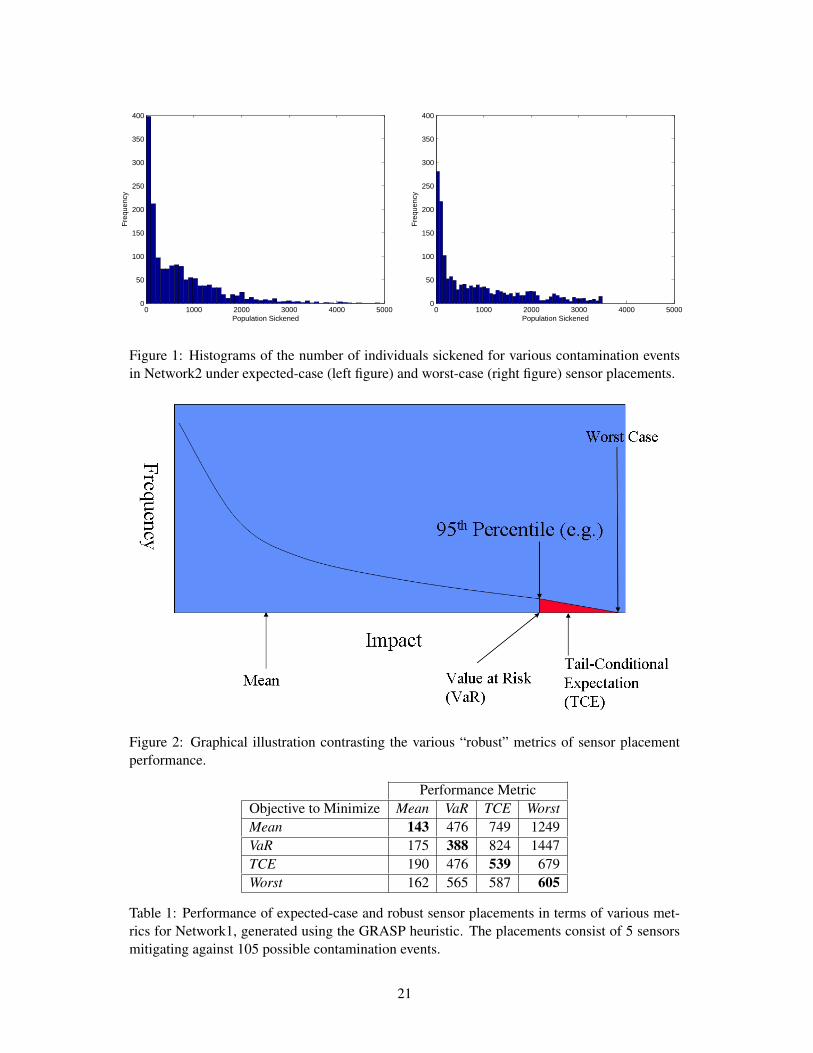
0 1000 2000 3000 4000 50000

50

100

150

200

250

300

350

400

Population Sickened

Fre

quen

cy

0 1000 2000 3000 4000 50000

50

100

150

200

250

300

350

400

Population Sickened

Fre

quen

cy

Figure 1: Histograms of the number of individuals sickened for various contamination eventsin Network2 under expected-case (left figure) and worst-case (right figure) sensor placements.

Figure 2: Graphical illustration contrasting the various “robust” metrics of sensor placementperformance.

Performance MetricObjective to Minimize Mean VaR TCE WorstMean 143 476 749 1249VaR 175 388 824 1447TCE 190 476 539 679Worst 162 565 587 605

Table 1: Performance of expected-case and robust sensor placements in terms of various met-rics for Network1, generated using the GRASP heuristic. The placements consist of 5 sensorsmitigating against 105 possible contamination events.

21

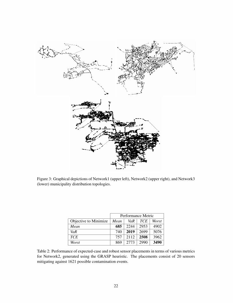
Figure 3: Graphical depictions of Network1 (upper left), Network2 (upper right), and Network3(lower) municipality distribution topologies.

Performance MetricObjective to Minimize Mean VaR TCE WorstMean 685 2244 2953 4902VaR 740 2019 2699 5076TCE 757 2112 2508 3962Worst 869 2773 2990 3490

Table 2: Performance of expected-case and robust sensor placements in terms of various metricsfor Network2, generated using the GRASP heuristic. The placements consist of 20 sensorsmitigating against 1621 possible contamination events.

22

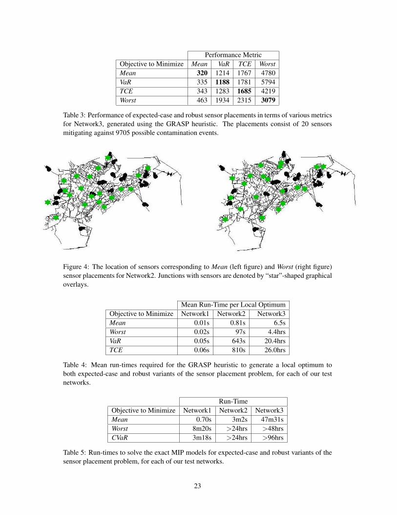
Performance MetricObjective to Minimize Mean VaR TCE WorstMean 320 1214 1767 4780VaR 335 1188 1781 5794TCE 343 1283 1685 4219Worst 463 1934 2315 3079

Table 3: Performance of expected-case and robust sensor placements in terms of various metricsfor Network3, generated using the GRASP heuristic. The placements consist of 20 sensorsmitigating against 9705 possible contamination events.

Figure 4: The location of sensors corresponding to Mean (left figure) and Worst (right figure)sensor placements for Network2. Junctions with sensors are denoted by “star”-shaped graphicaloverlays.

Mean Run-Time per Local OptimumObjective to Minimize Network1 Network2 Network3Mean 0.01s 0.81s 6.5sWorst 0.02s 97s 4.4hrsVaR 0.05s 643s 20.4hrsTCE 0.06s 810s 26.0hrs

Table 4: Mean run-times required for the GRASP heuristic to generate a local optimum toboth expected-case and robust variants of the sensor placement problem, for each of our testnetworks.

Run-TimeObjective to Minimize Network1 Network2 Network3Mean 0.70s 3m2s 47m31sWorst 8m20s >24hrs >48hrsCVaR 3m18s >24hrs >96hrs

Table 5: Run-times to solve the exact MIP models for expected-case and robust variants of thesensor placement problem, for each of our test networks.

23

B Pyomo Technical Report

30

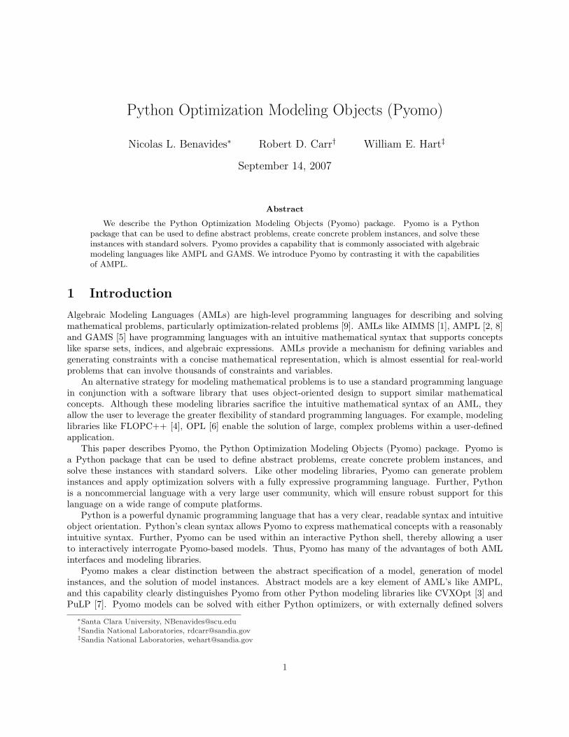
Python Optimization Modeling Objects (Pyomo)

Nicolas L. Benavides∗ Robert D. Carr† William E. Hart‡

September 14, 2007

Abstract

We describe the Python Optimization Modeling Objects (Pyomo) package. Pyomo is a Pythonpackage that can be used to define abstract problems, create concrete problem instances, and solve theseinstances with standard solvers. Pyomo provides a capability that is commonly associated with algebraicmodeling languages like AMPL and GAMS. We introduce Pyomo by contrasting it with the capabilitiesof AMPL.

1 Introduction

Algebraic Modeling Languages (AMLs) are high-level programming languages for describing and solvingmathematical problems, particularly optimization-related problems [9]. AMLs like AIMMS [1], AMPL [2, 8]and GAMS [5] have programming languages with an intuitive mathematical syntax that supports conceptslike sparse sets, indices, and algebraic expressions. AMLs provide a mechanism for defining variables andgenerating constraints with a concise mathematical representation, which is almost essential for real-worldproblems that can involve thousands of constraints and variables.

An alternative strategy for modeling mathematical problems is to use a standard programming languagein conjunction with a software library that uses object-oriented design to support similar mathematicalconcepts. Although these modeling libraries sacrifice the intuitive mathematical syntax of an AML, theyallow the user to leverage the greater flexibility of standard programming languages. For example, modelinglibraries like FLOPC++ [4], OPL [6] enable the solution of large, complex problems within a user-definedapplication.

This paper describes Pyomo, the Python Optimization Modeling Objects (Pyomo) package. Pyomo isa Python package that can be used to define abstract problems, create concrete problem instances, andsolve these instances with standard solvers. Like other modeling libraries, Pyomo can generate probleminstances and apply optimization solvers with a fully expressive programming language. Further, Pythonis a noncommercial language with a very large user community, which will ensure robust support for thislanguage on a wide range of compute platforms.

Python is a powerful dynamic programming language that has a very clear, readable syntax and intuitiveobject orientation. Python’s clean syntax allows Pyomo to express mathematical concepts with a reasonablyintuitive syntax. Further, Pyomo can be used within an interactive Python shell, thereby allowing a userto interactively interrogate Pyomo-based models. Thus, Pyomo has many of the advantages of both AMLinterfaces and modeling libraries.

Pyomo makes a clear distinction between the abstract specification of a model, generation of modelinstances, and the solution of model instances. Abstract models are a key element of AML’s like AMPL,and this capability clearly distinguishes Pyomo from other Python modeling libraries like CVXOpt [3] andPuLP [7]. Pyomo models can be solved with either Python optimizers, or with externally defined solvers

∗Santa Clara University, NBenavides@scu.edu†Sandia National Laboratories, rdcarr@sandia.gov‡Sandia National Laboratories, wehart@sandia.gov

1

(e.g. GLPK, CPLEX and CBC). Further, Python can integrate extension modules in low level languageslike C or C++ to directly leverage fast solver libraries, and wrapped modules can be used within Pythonexactly like native Python code.

Section 2 illustrates how Pyomo would be used to model a simple application. We compare and contrastthe Pyomo formulation with a formulation developed in the widely used AMPL modeling language. Section 3describes the Pyomo classes that are used to define model components.

2 A Simple Example

In this section we illustrate Pyomo’s syntax and capabilities by demonstrating how a simple AMPL examplecan be replicated with Pyomo Python code.

Consider the basic AMPL program prod.mod:

s e t P;

param a j in P ;param b ;param c j in P ;param u j in P ;

var X j in P ;

maximize To t a l P r o f i t : sum j in P c [ j ] ∗ X[ j ] ;

s ub j e c t to Time : sum j in P (1/ a [ j ] ) ∗ X[ j ] <= b ;

sub j e c t to Limit j in P : 0 <= X[ j ] <= u [ j ] ;

To translate this into Pyomo, the user must first import the Pyomo module and create a Pyomo Modelobject:

## Import Pyomo#from pyomo import ∗

## Create model#model = Model ( )

This import assumes that Pyomo is available on the users’s Python path (see Python documentation forPYTHONPATH for further details). Next, we create the sets and parameters that correspond to the dataused in the AMPL model. This can be done very intuitively using the Set and Param classes.

model .P = Set ( )

model . a = Param( index=model .P)model . b = Param( )model . c = Param( index=model .P)model . u = Param( index=model .P)

2

Note that parameter b is a scalar, while parameters a, c and u are arrays indexed by the set P . Pyomo alsodefines the ProductSet class, which can be defined in a similar manner.

Next, we define the decision variables in this model.

de f X bounds ( j , model ) :r e turn (0 , model . u [ j ] )

model .X = Var ( index=model .P, bounds=X bounds )

Decision variables and model parameters are used to define the objectives and constraints in the model.Parameters define constants and the variables are the values that are optimized. Parameter values aretypically defined by a data file that is processed by Pyomo.

Objectives and constraints are explicitly defined expressions in Pyomo. The Objective and Constraintclasses require a rule option that specifies how these expressions are constructed. This is a function thattakes one or more arguments: the first arguments are indices into a set that defines the set of objectives orconstraints that are being defined, and the last argument is the model that is used to define the expression.

de f Ob j e c t i v e r u l e ( model ) :ans = 0f o r j in model .P :

ans = ans + model . c [ j ] ∗ model .X[ j ]r e turn ans

model . p r o f i t = Object ive ( r u l e=Ob j e c t i v e r u l e )

de f Time rule ( model ) :ans = 0f o r j in model .P :

ans = ans + (1 . 0/ model . a [ j ] ) ∗ model .X[ j ]r e turn ans < model . b

model . Time = Constra int ( r u l e=Time rule )

The rules used to construct these objects use standard Python functions. Finally, note that the Time rulefunction includes the use of < and > operators on the expression. These operators are used to define upperand lower bounds on the constraints.

Once an abstract model has been created, it can be printed as follows:

p r i n t ’ ’ABSTRACT MODEL’ ’model . ppr int ( )

This summarize the information in the Pyomo model, but it does not print out explicit expressions. Thisis due to the fact that an abstract model needs to be instanted with data to generate the model objectivesand constraints:

i n s t ance = model . c r e a t e ( ’ ’ prod . dat ’ ’ )

p r i n t ’ ’MODEL INSTANCE’ ’i n s t ance . ppr int ( )

Appendix A shows the final Python code for this example.Once a model instance has been constructed, an optimizer can be applied to it to find an optimal solution.

For example, the PICO integer programming solver can be used within Pyomo as follows:

opt = s o l v e r s .PICO( path=”/home/wehart/ bin /PICO” , ke epF i l e s=True )s o l u t i o n s = opt . s o l v e ( i n s t ance )

3

This creates an optimizer object for the PICO executable defined in a given path, and it indicates thattemporary files should be kept. The Pyomo model is handed to this optimizer, which returns the finalsolutions generated by the optimizer.

3 Documentation of Pyomo Objects

In this section we provide more detail on the definitions of Pyomo classes that are used to define models.

3.1 Sets

The Set() class is used to index other objects (e.g. Param and Var). This class has the same look-and-feelas a sets.Set class, but it can be used to define an abstract set. This class contains a concrete set, whichcan be initialized by the load() method, or directly.

Constructor arguments:

• within - A set that defines the type of values that can be contained in this set

• default - Default set members, which may be overriden when setting up this set

• rule - A rule for setting up this set with existing model data. This has the functional form: f: py-omo.Model − > pyomo.Set

• restriction - Define a rule for restricting membership in a set. This has the functional form: f: data− > bool and returns true if the data belongs in the set

3.2 Product Sets

The ProductSet() class represents the cross product of other sets.

Constructor arguments:

• default - Default set members, which may be overriden when setting up this set

• rule - A rule for setting up this set with existing model data. This has the functional form: f: py-omo.Model − > pyomo.Set

• restriction - Define a rule for restricting membership in a set. This has the functional form: f: data− > bool and returns true if the data belongs in the set

In the following AMPL code, the rate paramater’s index set is the cross product of two sets:

s e t PROD;s e t STAGE;

param rat e PROD,STAGE ;

In Pyomo, the cross product is created with the ProductSet class, and the result of this is used to indexother Pyomo objects:

model .PROD = Set ( )model .STAGE = Set ( )

model . se tprod = ProductSet ( ( model .PROD, model .STAGE) )model . r a t e = Param( index=model . se tprod )steel4mod . ra t e > 0

4

3.3 Parameters

The Param() class defines constant values in a model, and a parameter object may be defined over an index.

Constructor arguments :

• index - The index set that defines the distinct parameters. By default, this is None, indicating thatthere is a single parameter.

• domain - A set that defines the type of values that each parameter must be.

• validate - A rule for validating this parameter with respect to data that exists in the model

• default - A set that defines default values for this parameter

• rule - A rule for setting up this parameter with existing model data

3.4 Variables

The Var() class defines a numeric variable, which may be defined over an index.

Constructor arguments:

• index - The index set that defines the distinct variables. By default, this is None, indicating that thereis a single variable.

• domain - A set that defines the type of values that each parameter must be.

• default - A set that defines default values for this variable

• bounds - A function that defines bound constraints for this variable

Simple bound constraints on variables can be specified with the bounds rule:

model .P = Set ( )

model . x lb = Param( index=model .P)model . x ub = Param( index=model .P)

de f x bounds ( i , model ) :r e turn ( model . x lb [ i ] , model . x ub [ i ] )

model . x = Var ( index=model .P, r u l e=x bounds )

3.5 Objectives

The Objective() class defines an objective expression.

Constructor arguments:

• rule - A rule for constructing this objective with existing model data.

• sense - Used to define wether this objective should be minimized or maximized (minimization is thedefault).

5

3.6 Constraints

The Constraint() class defines an expression whose value is constrained in the model.Constructor arguments:

• rule - A rule for constructing this constraint with existing model data.

• index - Defines a set of constraints over an index.

Note that the rule option generally needs to include a definition of the bounds on a constraint. Aconstraint must have either an upper or lower bound, and it may have both. For example:

model .P = Set ( )model .Q = Set ( )

model . x = Var ( index=model .Q)

de f c r u l e ( i , model ) :ans = 0f o r q in model .Q:

ans = ans + model . x [ q ]ans = ans > 0return ans < 1

model . c = Constra int ( index=model .P, r u l e=c r u l e )

The last two lines in the c rule function define upper and lower bound values for the c constraint. Notethat this is a non-standard use of the < and > operators; these operators return an expression rather thana boolean value.

3.7 Models

The Model() class defines a mixed-integer model that can be optimized by a user. This class takes noarguments, but it is a container for instances of the other Pyomo objects created by the user. For example,consider the statement:

model . x = Var ( )

This statement registers the variable x in the model, and assigns it the name “x”.

4 Conclusions

Pyomo has many of the features of abstract modeling languages and optimization modeling libraries, butthe following features of Pyomo are noteworthy:

• Pyomo supports the ability to define abstract problems from which problem instances can be generated.Further, Pyomo can generate multiple instances, which can be analyzed simultaneously in separatePython class objects.

• Pyomo is based on a powerful, commonly available open-source language. Thus, there are no licensinglimitations with the use of Pyomo, and the set of Pyomo objects can be customized for an applicationin ways that are not possible with commercial AMLs and modeling libraries.

• Python has a clean syntax, so Pyomo modeling objects can be used in an intuitive manner.

6

• Pyomo models can leverage Python’s programming language to define complex data structures andstandard programming constructs like classes and functions. Further, Python can be naturally linkedwith external libraries for high-performance kernels.

• Pyomo can integrate optimization solvers in an extensible manner. Optimizers can be defined withinPython itself, and external optimizers can be launched using file I/O to communicate with Python.1

Pyomo is probably most similar to the FLOPC++ modeling library. FLOPC++ is writen in C++, and ithas many of the same objects as are used in Pyomo. While FLOPC++ enables models to be embedded incompiled application codes, Pyomo enables the rapid prototyping of models in a scripting language. Thus,these capabilities seem quite complementary.

The current implementation of Pyomo has been validated on a small set of simple models. In the future,more extensive validation of Pyomo is needed to ensure that it can express a wide range of complex problems.Further, the performance of Pyomo needs to be analyzed to ensure that it can effectively generate large-scaleoptimization models. Finally, this document needs to be extended to include examples that illustrate howPyomo can leverage Python to develop complex models more naturally than AMLs like AMPL and GAMS.

This document describes the initial prototype of Pyomo. Once this code has stablized, we plan to integratePyomo into the COIN-OR optimization software repository to encourage its use within the academic andbusiness communities.

Acknowledgements

Thanks to Jon Berry and Cindy Phillips for their critical feedback on the design of Pyomo. Sandia is amultiprogram laboratory operated by Sandia Corporation, a Lockheed Martin Company, for the UnitedStates Department of Energy’s National Nuclear Security Administration under Contract DE-AC04-94-AL85000.

References

[1] AIMMS home page.

[2] AMPL home page.

[3] CVXOPT home page.

[4] FLOPC++ home page.

[5] GAMS home page.

[6] OPL home page.

[7] Pulp: A python linear programming modeler.

[8] R. Fourer, D. M. Gay, and B. W. Kernighan, AMPL: A Modeling Language for MathematicalProgramming, 2nd Ed., Brooks/Cole–Thomson Learning, Pacific Grove, CA, 2003.

[9] J. Kallrath, Modeling Languages in Mathematical Optimization, Kluwer Academic Publishers, 2004.

1For example, this is similar to the manner in which AMPL launches optimizers.

7

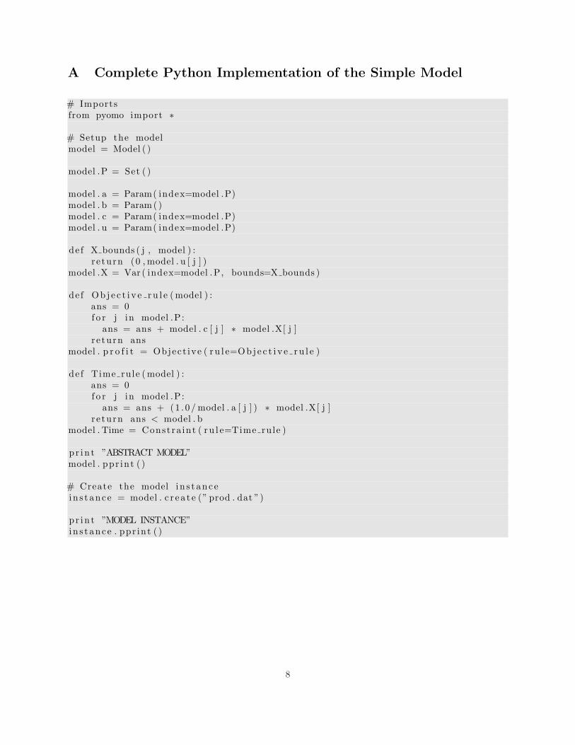
A Complete Python Implementation of the Simple Model

# Importsfrom pyomo import ∗

# Setup the modelmodel = Model ( )

model .P = Set ( )

model . a = Param( index=model .P)model . b = Param( )model . c = Param( index=model .P)model . u = Param( index=model .P)

de f X bounds ( j , model ) :r e turn (0 , model . u [ j ] )

model .X = Var ( index=model .P, bounds=X bounds )

de f Ob j e c t i v e r u l e ( model ) :ans = 0f o r j in model .P :

ans = ans + model . c [ j ] ∗ model .X[ j ]r e turn ans

model . p r o f i t = Object ive ( r u l e=Ob j e c t i v e r u l e )

de f Time rule ( model ) :ans = 0f o r j in model .P :

ans = ans + (1 . 0/ model . a [ j ] ) ∗ model .X[ j ]r e turn ans < model . b

model . Time = Constra int ( r u l e=Time rule )

p r i n t ”ABSTRACT MODEL”model . ppr int ( )

# Create the model i n s t ancein s t ance = model . c r e a t e (” prod . dat ”)

p r i n t ”MODEL INSTANCE”in s tance . ppr int ( )

8

DISTRIBUTION:

2 Regan MurrayUS EPA Facilities26 W Martin Luther King Dr (MS 163)Cincinnati OH 45268

1 MS 1316 Mark D. Rintoul, 14121 MS 1318 Robert D. Carr, 14121 MS 1318 Cynthia A. Phillips, 14121 MS 1318 Jean-Paul Watson, 14121 MS 1318 David Gay, 14111 MS 1318 Vitus Leung, 14151 MS 1318 Suzanne Rountree, 14151 MS 1318 David Womble, 14101 MS 1320 S. Scott Collis, 14141 MS 1320 Jonathan W. Berry, 14165 MS 1318 William E. Hart, 14122 MS 9018 Central Technical Files, 8944 (1 electronic, 1 hardcopy)2 MS 0899 Technical Library, 9536 (1 electronic, 1 hardcopy)1 MS 0123 D. Chavez, LDRD Office, 1011

31

32

v1.27