Embed Size (px)
Citation preview

I~ ~L~CONY
NAVAL POSTGRADUATE SCHOOLMonterey, California
ST AD-A219 909
5 ATELETEI Ilk
DTICELECTEMAR29 1990
THESIS U qEA LEVEL OF REPAIR MODEL
FOR THE INDONESIAN NAVY
by
Denny S. Partasasmita
September 1989
Thesis Advisor: Alan W. McMasters
Approved for public release; distribution is unlimited

SECURITY CLASSIFICATION OF THIS PAGE
Form ApprovedREPORT DOCUMENTATION PAGE OMB No, 0704.0188
la REPORT SECURITY CLASSIFICATION lb RESTRICTIVE MARKINGSUNCLASSIFIED None
2a SECURITY CLASSIFICATION AUTHORITY 3 DISTRIBUTION/AVAILABILITY OF REPORT
Approved for public release;2b DECLASSIFICATION /DOWNGRADING SCHEDULE distribution is unlimited.
4 PERFORMING ORGANIZATION REPORT NUMBER(S) S MONITORING ORGANIZATION REPORT NUMBER(S)
6a NAME OF PERFORMING ORGANIZATION 6b OFFICE SYMBOL 7a NAME OF MONITORING ORGANIZATION(If applicable)
Naval Postgraduate Scho 1 54 Naval Postgraduate School
6c. ADDRESS (City, State, and ZIP Code) 7b ADDRESS (City, State, and ZIP Code)
Monterey, CA 93943-5000 Monterey, CA 93943-5000
8a. NAME OF FUNDING I SPONSORING 8b OFFICE SYMBOL 9 PROCUREMENT INSTRUMENT IDENTIFICATION NUMBER
ORGANIZATION (If applicable)
8c. ADDRESS (City, State, and ZIP Code) 10 SOURCE OF FUNDING NUMBERS
PROGRAM PROJECT TASK WORK-UNITELEMENT NO NO NO 1ACCESSION NO.
11 TITLE (Include Security Classification)
A LEVEL OF REPATR MODEL FOR THE INDONESIAN NAVY
12 PERSONAL AUTHOR(S)
Partasasmita, Denny Supraden13a TYPE OF REPORT 13b TIME COVERED 14 DATE OF REPORT (Year, Month Day) 115 PAGE COUNT
Master's Thesis FROM TO September 1989 1 10316 SUPPLEMENTARY NOIATION The views expressed in this thesis are those of the author and donot reflect the official policy or position of the Department of Defense or the U.S.Government.17 COSATI CODES 18 SUBJECT TERMS (Continue on reverse if necessary and identify by block number)
FIELD GROUP SUB.GROUP -- Level of Repair Analysis; Maintainability; Weapon( systems; Indonesian Navy; Life-cycle costs): k -
19 ABSTRACT (Continue on reverse if necessary ahdjidentify by block number)I This thesis develops a mel'todology for making level of repair
decisions for new, fully devel6ped, weapon systems purchased by
the Indonesian Navy from other couihtries. This model considers
that Navy's current maintenance and ' upply organizations. Anexample illustrating the use of the mo'el is also presented.K_.J..J
20 DSTP BUjTiOI% AVALAB LTY OF ABS-RAC" 21 ABSTRACT SECUR'"
v CLASSi;,CATIOr,
r*')rCLASS- D i : -DFD 0 SA:E AS RPT 0 D71C USERS UNCLASSIFIED22a ,A"' OF PESOC " V D, A. 22b TELEPHONE (Include Area Code) 22C (i-FiCE SYMBOL
Alan W. Mc~as Ir (4nR)_ r6ir-9;7P T' t14j1_
DD Form 1473, JUN 86 Prevous editions are obsolete . i'- -ASS CATtO4 OF THIS PACE
SIN 0102-LF-014-6603 UNCLASSIFIEDi

Approved for public release; distribution is unlimited
A Level of Repair Model for The Indonesian Navy
by
Denny S. PartasasmitaCommander, Indonesian Navy
B.S., Indonesian Naval Electronic Academy, Bandung, 1967E.E., Indonesian Naval Institute of Technology, Jakarta, 1989
Submitted in partial fulfillment of the
requirements for the degree of
MASTER OF SCIENCE IN MANAGEMENT
from the
NAVAL POSTGRADUATE SCHOOL Accession ForNTIS GRA&I
Sep ember 1989 DTIC TABUnannounced QJustification
Author: /Den ny S. atsamt By
Partasasmita Distribution/
Availabilityode
Approved by: iAvail and/orDist Special
Alan W. McMasters, Thesis Advisor
Kent Alison, CDR, USN,S d Reader
f/fDavid R. WhippInDepartment of Administrate Sciences

ABSTRACT
This thesis develops a methodology for making level of repuic decisions for
new, fully developed, weapon systems purchased by the Indonesian Navy from other
countries. This model considers that Navy's current maintenance and supply orga-
nizations. An example illustrating the use of the model is also presented.
i'.

TABLE OF CONTENTS
INTRODUCTION ............................. 1
A. BACKGROUND ............................ 1
B. OBJECTIVE OF THE THESIS ................... 2
C. SCOPE OF THE THESIS ...................... 2
D. METHODOLOGY ........................... 2
E. RESEARCH QUESTIONS ...................... 3
F. LIMITATIONS AND ASSUMPTIONS ................ 3
G. PREVIEW OF THESIS ............ ............. 4
II. INDONESIAN NAVY'S LOGISTIC MANAGEMENT REVIEW ... 5
A. THE DEVELOPMENT OF MAJOR WEAPON SYSTEMS .... 5
1. The First Period (1950-1960) .................. 5
2. The Second Period (1961-1972) ................. 6
3. The Third Period (1973-1989) .................. 7
B. LOGISTIC SUPPORT MANAGEMENT ................ 8
C. OVERVIEW OF THE PRESENT MAINTENANCE ORGANI-
ZATION .................... .. ....... ... 12
D. THE NEED FOR MORE EFFECTIVE AND EFFICIENT MAN-
AGEMENT OF MAINTENANCE ................. 17
III. SYSTEM LIFE-CYCLE AND COST-EFFECTIVENESS RELATION-
SH IP . . . . . . . . . . . . . . . . . . . . . . . . . . . . . . . . . . . . 18
A. SYSTEM LIFE-CYCLE ........................ 18
B. COST-EFFECTIVENESS ....................... 20
1. System Effectiveness ....................... 23
v

2. Life-cycle Costs .............................. 30
C. LIFE SUPPORT COSTS IN RELATION TO MAINTENANCE
LEVEL ALTERNATIVES AND REPAIR/DISCARD DECISIONS 31
IV. THE FRAMEWORK OF LEVEL OF REPAIR ANALYSIS ...... 34
A. INTRODUCTION ..... ..................... 34
B. CLASSIFICATION OF EQUIPMENT INTO INDENTURE
LEVELS ................................ 36
1. Assumptions ............................ 38
2. Lim itations . . .. . . . .. . . . . . . .. . .. . . .. .. .. 38
C. EXISTING MAINTENANCE LEVELS OF THE INDONESIAN
N AVY . . . . . . . . . . . . . . . . . . . . . .. . . . . . ... . . . 39
D. THE OPTIMIZATION PROCEDURE ................ 42
E. THE COMPONENTS OF LIFE-SUPPORT COSTS ......... 44
1. Maintenance Manpower Cost .................. 46
2. Inventory Costs .......................... 49
3. Repair Material Costs ...................... 51
4. Support Equipment Costs .................... 52
5. Transportation Costs ....................... 54
6. Training Costs .......................... 55
V. AN EXAMPLE OF LOR ANALYSIS .................. 58
A. THE EXAMPLE SYSTEM ...................... 58
1. System Configuration of the Example ................ 58
2. Input Data Requirement ..................... 61
B. LIFE-SUPPORT COST COMPUTATION .............. 64
1. Discard Alternative ........................ 67
2. Depot Alternative ........ ................ 67
vi

3. Intermediate Alternative ......................... 68
4. Total Cost for Assembly 1.2 (WRA) ................. 69
5. Total Cost for Assembly 1.2.1 (SRA) ................. 70
6. Total Cost for Assembly 1.2.2 ...................... 70
7. Total Cost for Assembly 1.2.2.1 .................... 70
8. Total Cost for Assembly 1.2.2.2 .................... 70
VI. SUMMARY, CONCLUSIONS, and RECOMMENDATIONS ...... .73
A. SUMMARY ...... .............................. 73
B. CONCLUSIONS .................................. 73
C. RECOMMENDATIONS ............................. 74
APPENDIX A - The Possible Alternatives of LOR Assignment ......... 76
APPENDIX B - Total Life Cycle Costs for the LOR Alternatives for the Driver
Assem blies . . . . . . . . . . . . . . . . . . . . . . . . . . . . . . . . . . . . . 78
APPENDIX C - A Glossary of Abbreviations and Acronyms ........... 83
LIST OF REFERENCES ............................. 86
INITIAL DISTRIBUTION LIST ......................... 87
vii

LIST OF TABLES
2.1 Number of Ships Managed by Three Unit Commands ........... 13
5.1 Poisson Probability Distribution for Computing Ncd ........... 66
5.2 Values of Ncd, Nci, and Nco ........................... 66
VIII

LIST OF FIGURES
2.2 Organizational Structure of Fleet Maintenance Management in the
Indonesian Navy ...... ............................. 16
3.6 Life-cycle Costs [Ref. 10:p. 19] .......................... 31
4.1 Equipment Indenture Levels ........................... 37
4.2 LOR Code Assignment Procedure [Ref. 12:p. 110] ............. 40
5.1 Example System Configuration ......................... 59
5.2 LOR Code Assignment Possibilities ....................... 60
ix

I. INTRODUCTION
A. BACKGROUND
The rapid advances in technology which have occurred since the end of World
War II have led to the design of systems of increasing complexity. As a consequence
the problem of maintenance support is also becoming more complicated and difficult
to perform. Increased complexity of system design appears to be inevitable as new
missions are defined and as higher performance requirements are specified.
Considerable resources have been expended on research on improving sys-
tem reliability. Reliability directly influences the need for preventive maintenance
and repair. The achievement of increased reliability may simultaneously require an
increased demand on the maintenance technician in terms of skill, training, and
maintenance man-hours, and on the logistics pipeline in terms of spares or repair
parts. The consequence is increasing logistic support cost.
During the last decade costs associated with system/product acquisition and
logistic support have increased at an alarming rate. At the same time decreasing
government budgets combined with inflationary trends have resulted in less -money
being available-for procurement of new systems-and for the maintenance and support
of those systems already in use. This requirement to increase overall productivity in
a resource-constrained environment has forced -attention to all aspects of a system's
life-cycle. The system's life-cycle costs must be given more attention, particularly
those costs associated with system operation and support since these costs often
constitute a major portion of the total life-cycle costs.

In the U.S. Navy weapon systems are evaluated from the support point-of-
view from their conception. The sources of high support costs are addressed as part
of design. The goal is to minimize maintenance costs without sacrificing system
operational effectiveness.
The Indonesian Navy, like other navies of developing countries, is not involved
in design development. Instead, it uses systems developed by major countries like
the United States. With such systems comes the need for maintenance. How best
to perform this maintenance is the problem. Since a significant portion of the
Indonesian Navy's budget goes to support such weapon systems, improvement in
logistic support management of such systems by the Indonesian Navy is considered
to be very important.
B. OBJECTIVE OF THE THESIS
The purpose of this thesis is to develop a methodology for making level of
repair (LOR) decisions for new weapon systems which have-been developed by other
countries and are going to be purchased from them by the Indonesian Navy. The
objective of this methodology is to allow the existing maintenance organization of
the Indonesian Navy to accomplish the required maintenance at least cost.
C. SCOPE OF THE THESIS
The current application of LOR decisions by the U.S. Navy will be studied to
structure a specific model of repair analysis that can be applied in the Indonesian
Navy's existing organization.
D. METHODOLOGY
The methodology developed in this thesis will be predominantly an extension
of the LO1 analysis currently in the literature. A comparison of the planning for
2

logistics by the Indonesian Navy with that of the U.S. Navy will be needed as the
first part of model development.
E. RESEARCH QUESTIONS
The author seeks answers to the following research questions:
1. How can LOR models be used for weapon systems that have already been
designed?
2. How can the LOR decisions incorporate the existing maintenance organization
of the Indonesian Navy?
3. Is there any -possibility that the least total maintenance costs can be achieved
with LOR analysis on existing weapon systems?
4. What cost analysis model structure will ensure the least total life-cycle main-
tenance cost?
5. What are the problems, if any, with applying this limited LOR analysis to the
weapon systems being purchased for the Indonesiar Navy?
F. LIMITATIONS AND ASSUMPTIONS
Unfortunately, a major factor that limited the research effort was the scarcity
of Indonesian Navy df -. This scarcity is caused by the weak communications link
between the United States and Indonesia. In addition, the author experienced re-
strictions on access to certain U.S. documents because of their security classification.
These constraints might afrect the validity of the analysis.
:3

The following assumptions are used in the analysis to follow:
1. No changes have occurred in the policy of the Indonesian Navy associated with
logistic support management during the period from 1987 to 1989. Thus, the
knowledge of the author, gained prior to 1987, is assumed to be correct.
2. The equipment to be analyzed in the example is a simplified configuration of
a typical component of an existing weapon system.
G. PREVIEW OF THESIS
In Chapter II the author traces the evolution of the Indonesian Navy since
World War II to provide insight about the management, policies and planning for
logistics used by the Indonesian Navy. Chapter III then introduces the reader to
the concepts of system -life-cycle, system effectiveness, life-cycle costs and cost-effec-
tiveness analyses.
Chapter IV proposes a model for LOR analysis which incorporates the existing
maintenance organization of the Indonesian Navy. A procedure for determining the
lowest life-support cost alternative is also described.
Chapter V describes an example application of the model developed in Chapter
IV. The details of the computations of the life-support costs for the alternative
maintenance levels are-described.
Chapter VI presents a summary of the thesis, and its conclusions and recom-
mendations.
4

II. INDONESIAN NAVY'S LOGISTICMANAGEMENT REVIEW
A. THE DEVELOPMENT OF MAJOR WEAPON SYSTEMS
The evolution of major weapon systems in the Indonesian Navy since World
War II will be reviewed to provide insight into the general structure of the orga-
nizations responsible for the logistic support management of such systems. This
evolution will be divided into three periods corresponding to the major changes in
the management effort.
1. The First Period (1950-1960)
The first period was during and immediately after the Indonesian War
of Independence. The Indonesian Navy began its ship acquisition by transferring
some ships from the Federal Schepedienst, Netherlands East Indies [Ref. l:p. 24].
After the War of Independence, the Indonesian Navy expanded its fleet
with acquisitions from Italy, U.S.A., U.S.S.R., West Germany, Yugoslavia, and
Japan. During this period, the Indonesian Navy bought frigates, corvettes, and
submarines for the first time. The first submarines were purchased from Poland and
transferred to the Indonesian Navy in August 1959.
Under the Mutual Defense Assistance Program, the Indonesian Navy
bought submarine-chasers and landing ship transports from the United States.
Under the government of the Netherlands East Indies, the shipyards DROOG-
DOK MAATSCHAPPIJ, Jakarta, and DROOGDOK MAATSCOHAPPIJ, Surabaya,
produced three auxiliary minesweepcrs (175 tons) and finished another auxiliary

minesweeper of the same type which was started during the Japanese occupation
[Ref. 2:p. 63]. These ships were the resilt of Dutch shipbuilding technology.
During this period, maintenance activities were designed to meet the
operational requirements without any major distinction between the levels of main-
tenance. These maintenance activities were a consequence of very limited budgets,
few adequately trained personnel, limited test equipment, and poor supply support
[Ref. 3 :p. 29].
2. The Second Period (1961-1972)
This period witnessed the largest number of acquisitions of the weapon
systems that has ever occurred in the Indonesian Navy. These acquisitions occurred
in conjunction with the return of West Irian (West Papua) to the Republic of In-
donesia. These acquisitions produced a number of benefits for Indonesia, including:
improved defense of the long coast line, safeguarding of offshore oil installations, and
transfer of technology to the Indonesian Navy. During this period the Indonesian
Navy developed the ability to operate and utilize modern weapon systems and, at
the same time, acquired the skill to maintain all system components. As in the
first period maintenance activities were designed to meet operational requirements
with no major distinctions being made between levels of maintenance. During this
period almost all corrective maintenance actions were effectively performed for the
first time because all ships' crews had received at least one year of training in such
maintenance actions in the U.S.S.R.
Following the period from 1965 to April of 1967, during which all Indone-
sian military procurements were suspended, a new government was formed. During
this second period the Indonesian Navy purchased no ships from the United States
until after April 1967. The new Indonesian government requested that the United
States help develop the Indonesian Armed Forces [Ref. 2 :p. 65].
6

3. The Third Period (1973-1989)
During this period the Indoresian government, headed by President Su-
harto, rebuilt the Indonesian Armed Forces. Because some of the equipment and
ships acquired from the U.S.S.R. were inoperable, and spares and replacement parts
were unavailable, many of them had to be scrapped.
At the beginning of this period, the Indonesian Navy bought four used
frigates, of the former U.S. "CLAUDE JONES" class, which were commissioned
in 1973 and 1974. At the same time the Indonesian Navy ordered several U.S.
designed patrol boats from Korea. In 1975 it bought three new corvettes from
the Netherlands (commissioned in 1979). A project management organization was
formed for this acquisition and was located in Wilton Fijenoord, Shiedam, Nether-
lands. The Indonesian Navy task force was helped by the Royal Netherlands Navy
(KONINGLIJKE MARINE).
In 1979 two submarines were purchased from West Germany through the
assistance of the West German Navy (BUNDESWHER MARINE). In 1985 tbree
frigates-of the ex-BRITISH "'RIBAL" class were purchased and commissioned by
the Indonesian Navy. In 1986, 1987 and 1988, three used frigates were purchased
from the Netherlands and modernized [Ref. 4:pp. 255-259]. During this period
a majority of the current logistics management and maintenance methods were
introduced by the Dutch Navy since most of the modern ships acquired by the
Indonesian Navy were purchased from the Netherlands. In addition, all of the
ships' crews and base maintenance personnel received on-the-job training in the
Netherlands.
In 1980 Indonesia established a 20-year strategic plan to develop a Navy
of 25,000-seamen and 5,000 marines to man a fleet that would include four fast A/S
frigates, six submarines, six light fast attack craft (missile, gun and torpedo), six
7

minelayers, six minesweepers, a fast headquarters ship, a fast supply ship, and one
or two more corvettes. Additional plans in 1986 added six more submarines and
three more frigates to the plan. The construction of those three frigates has begun.
The acquisition of five more frigates, two submarines, four fast attack craft (missile),
a new patrol craft and a new training ship has been completed. All major surface
ships are also being fitted with missiles.
Indonesia now has nine shipbuilding yards (seven private and two govern-
ment-owned) and is in a position to build its own ships up to frigate size. Requests
for proposals have been sent to 13 industrial countries' firms for the design of 2300-
2800 ton frigates (details must be submitted by the end of this year). In all, 23 ships
are planned, the first two to be built in the selected designer's yard, the remainder
at P.T. Pal (a private shipyard company), Surabaya, Indonesia, over the next 30
years [Ref. 4:p. 255].
B. LOGISTIC SUPPORT MANAGEMENT
In 1985 to achieve greater effectiveness and efficiency the Indonesian Navy
reduced the number of its unit commands to only a few by consolidating some and
liquidating others. Some of the management publications issued by the Indonesian
Navy, such as management guides, regulations, and directives, as well as a logistic
support management guide, have been revised to incorporate the structure and
requirements of the new organization. At the beginning of 1987 the Indonesian Navy
issued a new logistics management guide called "Pola Pembinaan Bidang Materil,
PUM-1.03" [Ref. 5:pp. 1-30]. PUM-1.03 is a general guide for managing Naval
material and logistic support. The major change is the Navy's maintenance policy
that depot mainte',ance for Naval ships will be performed by shipyard contractors
S

[Ref. 5:p. 23]. The Indonesian Navy has selected six shipyards (four private and
two government owned). These will be listed in the next section.
The main objective of logistic support management of the Indonesian Navy
is to support the integrated weapon systems (SSAT). The SSAT (Sistim Senjata
Armada Terpadu) is defined by the Indonesian Navy as the integration of four force
components:
1. SHIPS
2. AIRCRAFT
3. MARINE CORPS
4. NAVAL BASES (Naval Harbors)
Since Indonesia is an archipelagic country, many Naval bases are required throughout
the country. There are-ten Naval bases in Indonesia at present. For this reason Naval
bases are included in the four components.
The Indonesian Navy applies an integrated logistic support concept to weapon
systems during the provisioning process before initiation of the -program whenever
possible, and throughout the life-support phase (operational-use-phase). Application
of integrated logistic support to only the operational-use phase is-for weapon systems
that have already been designed without the Indonesian Navy's involvement in the
design process.
Basically, material and logistic management in the Indonesian Navy consists
of eight functions [Ref. 6:pp. 25-26]:
1. Material requirement determination
2. Procurement
9
3. Inventory
4. Maintenance
5. Information systems
6. Material distribution
7. Disposal
8. Standardization
In the organizational structure of the Indonesian Navy, four directorates deal
with logistics and material management, as illustrated in Figure 2.1 [Ref. 7 :p.
56]. The four directorates are under the control of the Deputy Chief of the Naval
Staff-Logistics. In addition, there are three unit commands within the organization
responsible for managing the ships. These are the Eastern Fleet Command, headed
by the Commander-in-Chief Eastern Fleet, located at the Naval base at Ujung,
Surabaya East Java; the Western Fleet Command, headed by the Commander-
in-Chief Western Fleet, located at Jakarta, West Java; and the Military Sea Lift
Command, headed by the Commandant of Military Sea Lift, located at Naval base
at Tanjung Priok, Jakarta. In dealing with logistic and material management, each
unit command has its own organizational structure.
10

CHIEF OFTHE NAVAL STAFF
11IDEPUTY LOGISTICS
DIRECTOR, DIRECTOR, DIRECTOR, DIRECTOR,MATERIAL NAVAL BASE SUPPLY PROCUREMENT
FACILITIES
EASTERN WESTERN MILITARY MARINEFLEET FLEET SEA LIFT [CORPS
Figure 2.1: Organizational Structure of Logistics Management in the
Indonesian Navy [Ref. 7 :p. 56]
The development of the Western Fleet began in 1985 in conjunction with the
new organization of the Indonesian Navy, and is still evolving. The Naval -base for
the Western Fleet, being built at Teluk Ratai, South Sumatra, is expected to be
finished in the near future.
The Indonesian Navy must support both old and new ships which have been
purchased from different countries. The approximate number of ships managed at
11

present by the three unit commands described above are listed in Table 2.1 [Ref.
4:p. 255].
Additional ships to be purchased under the present plan are one frigate, six fast
attack craft (gun/torpedo), six hydrofoils, two main warfare vessels, and two main-
sweepers [Ref. 4:p. 255].
C. OVERVIEW OF THE PRESENT MAINTENANCE ORGANIZA-
TION
For preventive maintenance, maintenance management prepares a mainte-
nance plan and schedule for each "new" ship [Ref. 3:p. 31]. This method was
initiated in the third period when the Indonesian Navy began acquiring modern
systems such as new ships from the Netherlands and West Germany. All weapon
systems on each ship are provided with a maintenance schedule. For example, a
ship's systems may have a maintenance schedule which consists of daily inspection;
weekly, monthly or quarterly maintenance; and major overhauls every two years.
Each ship has been projected to accomplish a specific mission, depending on
the operational requirements needed and planned [Ref. 3:p. 31]. Based on these
operational requirements, the Indonesian Navy determines the maintenance plan for
each ship.
Corrective maintenance activities are basically organized into three levels [Ref.
5:p. 23]:
1. Organizational maintenance, performed by the using organization;
2. Intermediate maintenance, performed by a Naval base's maintenance facility;
3. Depot maintenance, performed by the designated shipyard contractor.
12

TABLE 2.1: Number of Ships Managed by Three Unit Commands
TYPE NUMBER
Patrol Submarines 2
Frigates 14
Fast Attack -Craft (Missile) 4
Fast Attack Craft (Gun/Torpedo) 2
Large Patrol Craft 12
Coastal Patrol Craft 8
Hydrofoils 5
LST's 15
Amphibious Craft 62
Minesweepers 2
Survey Ships 9
Submarine Tenders 2
Replenishment Tankers 1
Harbor Tankers 5
Cable Ships 1
Tugs 6
Training Sailing Ship 1
Miscellaneous 23
13

At present, because of the sophistication of the systems being maintained
and an inadequate number of technical personnel, the only maintenance actions
performed at the organizational level are replacements [Ref. 3:p. 34].
The maintenance functions at the depot level are performed by the shipyards
selected by the Indonesian Navy. The Indonesian Navy has designated six shipyards
to perform depot maintenance:
1. Perusahaan Terbatas (PT) Pal Indonesia shipyard
2. Perusahaan Negara (PN) Dok Jakarta shipyard
3. Perusahaan Negara (PN) Dok Surabaya shipyard
4. Perusahaan Terbatas (PT) Pelita Bahari shipyard
5. Perusahaan Terbatas (PT) Kodja shipyard
6. Perusahaan Terbatas (PT) Intan Sengkunyit shipyard
"Perusahaan Terbatas (PT)" refers to a private company, and "Perusahaan Negara
(PN)" refers to a government owned shipyard.
The only Navy owned supply facility is the Inventory Storage Center which is
available to support depot maintenance. There are two Inventory Storage Centers,
one for the Naval Eastern Region, located at Surabaya, East Java, and the other for
the Naval Western Region, located at Jakarta, West Java. The function of -the In-
ventory Storage Center is to provide spare parts and material for-depot maintenance
activities performed at the contractor facilities [Ref. 5:p. 25].
Spare parts needed for intermediate and organizational maintenance are -being
stocked at intermediate and organizational maintenance facilities.
14

The Indonesian government hopes that the shipyard contractors will expand
after acquiring experience in maintaining and repairing a combat ship. In addition,
it is hoped that the repair time might be shorter than it was previously when
performed by Navy personnel.
The structural organization of the Fleet Commands associated with mainte-
nance management is illustrated in Figure 2.2. Maintenance management in the
Eastern and Western Fleets is performed by the Fleet Maintenance Department,
and in the Military Sea Lift Command by the Material Department, under the su-
pervision of Assistant Commandant, logistics staff. Intermediate maintenance is
performed at each Base Maintenance Facility by the Base Maintenance Team.
Three additional teams, appointed annually, are associated with maintenance
activities:
1. SHIP-CHECK TEAM
2. NEGOTIATION TEAM
3. LIAISON OFFICERS
The Ship-Check Team's function is to investigate failed items to determine
the spare parts required for repairing them and to make a proposal to the Chief
of the Fleet Maintenance Department regarding whether the failed item should be
repaired at the intermediate or at the depot level. These actions are done quarterly
and before major overhauls [Ref. 3:p. 31].
One of the Negotiation Team's functions is to calculate the Navy standard
maintenance costs of the failed items and the costs of spare/repair parts that should
be procured if not available in inventory. The team then compares these costs with
those proposed by the contractor I negotiates these costs if they are considered
to be too high.

COMMANDER-IN-CHIEF *FLEET COMMAND
ASSISTANT COMMANDER, **LOGISTICS STAFF
CHIEF OFFLEET MAINTENANCE
DEPARTMENT
CHIEF OFBASE MAINTENANCE
FACILITY
Note:For Military Sea Lift Command,* = Commandant
** = Assistant Commandant, Logistics Staff
= Chief of Material Department
Figure 2.2: Organizational Structure of Fleet Maintenance Management
in the Indonesian Navy
16

The liaison officers' functions are to monitor the progress of depot maintenance
activities performed at the shipyard contractor's facility and to advise the contractor
and Chief of the Fleet Maintenance Department about problems encountered during
depot maintenance.
One of the most important tasks performed by the three teams is to find pos-
sible cost savings without sacrificing effectiveness. Since sophisticated cost analysis
using trade-off studies, present value of money, and inventory models, etc., have not
been conducted yet, it is sometimes difficult to achieve this goal satisfactorily.
D. THE NEED FOR MORE EFFECTIVE AND EFFICIENT MAN-
AGEMENT OF MAINTENANCE
Since major weapon systems have become more complex as technology has
advanced, logistics requirements in general have increased. At the same time de-
creasing budgets combined with upward inflationary trends have resulted in less
money being available for maintenance and support of systems already in use.
One of the greatest challenges facing the Indonesian Navy today is the growing
need for more effective and efficient management of resources. Experience has indi-
cated that operation and maintenance costs constitute a large portion of the Navy's
budget. The Indonesian Navy, like navies of other developing countries which usu-
ally buy fully developed weapon systems, is primarily concerned with the use period
of life-cycle support. However, at the beginning of the use period there is an op-
portunity for the Indonesian Navy to perform life-support cost analysis relative to
repair or discard decisions and maintenance level alternatives. The objective of this
analysis is to minimize life-cycle maintenance costs. Models to perform this analysis
are the subject of the following chapters.
17

III. SYSTEM LIFE-CYCLE ANDCOST-EFFECTIVENESS RELATIONSHIP
A. SYSTEM LIFE-CYCLE
A basic knowledge of the system life-cycle concept is fundamental to an un-
derstanding of the cost-effectiveness approach to be presented in this thesis. It is
during the early phases of the system life-cycle that a system's effectiveness char-
acteristics are determined, and these establish the quantitative basis for trade-offs
between subsequent effectiveness and cost elements [Ref. 8:p. 19].
Any system is designed and produced to satisfy a need. Moreover, the system
must be able to continue to meet the need over a specified period of time to justify
the investment in time, money, and effort. Thus, one must consider a system in
a dynamic sei,se-that is, from a life-cycle or so-called "cradle-to-grave" viewpoint
[Ref. 8:p. 191.
The system life-cycle represents the phases through which any system passes,
as well as the activities that take place during these phases.
The system life-cycle, as illustrated in Figure 3.1, starts with the Planning Pe-
riod, during which the need for a new system is verified and system operational and
maintenance concepts are formulated. The operational and maintenance environ-
ments and resources available are considered, and system feasibility is determined by
consideration of operational, technological, economic, political, legal, and other fac-
tors. At the end of this period, the system is defined by a set of design requirements
to meet operational needs [Ref. 8:p. 21].
1s

CONCEPT FORMULATION
PHASEII PLANNING
OPERATIONAL AND MAINTENANCE PERIODREQUIREMENTS (U ER)
[ SYSTEM DEFINITIONPHASE
SYSTEM R QUIREMENTS
DESIGN PHASE
ACQUISITIONPERIOD
(PROD CER)PRODUCTION AND
INSTALLATION PHASES
I OPERATION ANDSUPPORT PHASE
USEPERIOD
____ ___ __ ____ ___ ___(US R)
MODIFICATION AND 1RETIREMENT PHASES
Figure 3.1: System Life Cycle [Ref. 8:p. 163]
The Acquisition Period includes the-design, test, evaluation, production, and
installation of the system. It is during the-design phase that the-effectiveness charac-
teristics, specified as a-set of requirements-in the previous period, are converted into
a hardware system -that can be tested and verified. Some redesign and modification
19

of the system is often needed as a result of these tests. Prior to production, system
specifications previously agreed upon by the customer and producer are demon-
strated or modified as a result of a cost-effectiveness evaluation. The effectiveness
value achieved and cost estimate for the system's operational period (e.g., opera-
tional availability and life support cost) must be accepted by both parties [Ref. 8:p.
22].
The Use Period includes all operation and support activities. This is the
longest and most expensive period of the life-cycle. Sometimes changes are intro-
duced into the system during this period as a result of problems detected from actual
use in an operational environment. The Use Period ends with retirement of the sys-
tem from active service because operation and support are no longer co.st-effective.
The requirements for sustaining a system day-to-day are initially identified
through the maintenance concept, and subsequently refined through logistic sup-
port analysis (LSA). The results of LSA, in terms of maintenance levels, personnel
quantities and skills, and test and support equipment, are usually included in an
integrated logistic support plan prepared before the start of the production phase
and used as a basis for implementing a life-cycle support capability for the system
throughout its operational-use phase.
B. COST-EFFECTIVENESS
The development of a system that is cost-effective, within the constraints spec-
ified by operational and maintenance requirements, is a prime objective. Cost-
effectiveness analyses provide a conceptual framework and methodology for the sys-
tematic investigation of alternatives. Determining cost-effectiveness involves mea-
suring each alternative in terms of cost (total expenditure during the life-cycle)
20

versus effectiveness (level of mission fulfillment). By applying this analysis proce-
dure, it is possible to select the optimal alternative for achieving of the goals defined
within the allowed constraints [Ref. 8:p. 23].
Of the two elements-cost and effectiveness-cost is easier to measure and han-
dle because it can be expressed by a single monetary value. Effectiveness can be
presented both in terms of certain parameters that have a clear-cut numerical rep-
resentation and others that are not readily quantifiable.
Cost-effectiveness analyses, which are similar to the standard cost-benefit anal-
yses employed in many industrial and business applications, can be expressed in
various terms (i.e., one or more figures of merit) depending on the specific mis-
sion or system parameters that one wishes to measure. The prime ingredients of
cost-effectiveness are illustrated in Figure 3.2 [Ref. 10:p. 20].
21

LeyCost-Effectiveness
S Life-Cycle System 1
Cost E Effectiveness
*Research and Availa- Dependa- SystemIDevelopment Cost bility bility Performance Others*Investment Cost*Operation andMaintenance Cost*System phaseoutCost
Design Attributes Logistic Support Elements
Functional Design Maintenance Planning
Reliability Test & Support Equipment
Maintainability I Spare Repair/Parts
Human Factors Personnel & Training
Producibility Technical Data
Othes IFacilities
ITransportation & Handling
Figure 3.2: Basic Ingredients of Cost-Effectiveness [Ref. 10:p. 20]
22

I
1. System Effectiveness
According to Blanchard [Ref. 10:p. 18], system effectiveness is often
expressed as one or more figures of merit representing the extent to which the
system is able to perform the intended function (see Figure 3.2). The figures of
merit used may vary considerably depending on the type of system and its mission
requirements. Figures of merit may include [Ref. 10:p. 18]:
System Performance Parameters, such as the capacity of a power plant, rangeor weight of an airplane, destructive capability of a weapon, quantity of lettersprocessed through a postal system, amount of cargo delivered by a transfor-mation system, and the accuracy of a radar capability.
Availability, or the measure of the degree of a system is in the operable andcommittable state at the start of the mission when the mission is called forat unknown random point in time. This often called "operational readiness".Availability is a function of operating time (reliability) and downtime (main-tainability/supportability).
Dependability, or the measure of the system operating condition at one ormore points during the mission, given the system condition at the start of themission (i.e., its availability). Dependability is a function of operating time(reliability) and downtime (maintainability/ supportability).
System effectiveness is used as a predictive tool during the planning and
design phase of the life-cycle, and should be evaluated continually as system devel-
opment proceeds to insure obtaining an objective measure of fulfillment of system
needs.
Of the three figures of merit listed above, availability is the most com-
monly used in military situations. There are three types of availability: inherent,
achieved, and operational. The one considered most important for effectiveness
evaluation purposes during the system's Use Period is operational availability (Ao)
23

since it is more closely related to the actual operational environment than the other
two measures and is affected more by user decisions.
Operational availability can be defined as [Ref. 10:p. 65]:
The probability that a system or equipment, when used under stated condi-tions in an actual operational environment, will operate satisfactorily whencalled upon.
Operational availability can be expressedI as:
A 0 =MTBMAo = IBA
MTBM + MDT
where
MTBM = mean time between maintenances, and
MDT = mean maintenance downtime.
When preventive maintenance downtime is not considered, MTBM be-
comes MTBF (mean time between failures), and operational availability can be
expressed as [Ref. lI:p. 26]:
MAITBF
MTBF + MDT
As stated above, availability concerns itself with operating time (reliability) and
downtime (maintainability/supportability).
In dealing with maintenance problems, one must understand the concept
of reliability. System reliability is usually expressed as a probability, and can be
defined as [Ref. 10:p. 23]:
The probability that a system or product will perform in a satisfactory mannerfor a given period of time when used under specified operating conditions.
24

A basic concept in reliability is the "Bathtub Curve" (see Figure 3.3),
which represents the instantaneous failure rate. It consists of three regions: "infant
mortality" where the failure rate is decreasing, constant failure rate, and "wearout
region" where the failure rate is increasing. In the constant failure rate region, the
times to failure can be described by an exponential distribution. In this region, the
reliability over time t can be expressed as:
R = e-t =
-t/MTBF
where
= Time period of interest (t > 0);
A = Instantaneous failure rate or frequency of corrective maintenance;
and
MTBF = Mean time between failures -1
In- determining system support requirements, the frequency -of corrective
maintenance (A), or its inverse, MTBF, becomes a significant parameter. In general,
as the reliability of a system increases, the MTBF will increase. Conversely, the
MTBF will decrease as system reliability is degraded.
The second parameter of system availability is maintenance downtime
(MDT) which is a function of maintenance and support activities. Maintenance
involves activities directed toward failure prevention (preventive maintenance) and
failure correction (corrective maintenance). A commonly used definition of mainte-
nance is [Ref. 9:p. 63]:
All actions necessary for retaining an end item in, or restoring it to,-a service-able condition.
25

Failure Decreasina Constant- failure Increasingrate failure rate rate region failure rate
region duringI (Exponential during"debugging" failure law "wearoutit
Iapplies)I
I I
Component life
Figure 3.3: Typical Failure-Rate Curve [Ref. 10:p. 28]
26

Preventive or scheduled maintenance is often referred to as "retaining,"
while corrective maintenance is often referred to as "restoring." Preventive main-
tenance, on a scheduled basis to retain an item in satisfactory operating condition,
includes servicing and inspection activities. Planning preventive maintenance in-
volves selecting the manpower necest;ary to maintain the system, determining the
time between periodic system inspections, and selecting items to receive preventive
inspection at each succeeding period. All three activities should be combined to yield
the least cost maintenance condition for the level of system operation required.
Corrective maintenance is that maintenance performed to return an equip-
ment to service after a failure or other malfunction has occurred. It includes fault
detection, diagnosis, correction,- and verification.
The relationships among the primary subsets of preventive and corrective
maintenance are illustrated in Figure 3.4 [Ref. 9:p. 54]. A further partitioning of
corrective maintenance activities results in the identification of the more elementary
tasks involved, including the secondary maintenance loop for rear echelon repair of
removed items. These are illustrated in Figure 3.5 [Ref. 13:p. 55].
Maintenance downtime can be expressed as the sum:
MDT = 1 + ADT + LDT
where A1 = Mean active maintenance time (sensitive to environment, technician
skill level, procedures, etc.);
ADT = Administrative delay time (sensitive to administrative proce-
dures, filing, storage, etc.); and
LDT = logistic delay time (time used in obtaining spares or repair parts
or in waiting for personnel, manuals, tools, or test equipment).
27

MAINTENANCE
PREVENTIVE CORRECTIVEMAINTENANCE MAINTENANCE
SERICEINSPECTION DETETION l
DETECTED > IGOSI
CORTIOZN~
ACCEP TABLEX SYSTEM
Figure 3.4: The Primary Subsets of Maintenance [Ref. 9 :p. 54]
28

FAILURE
OCCURS
FAILURE IS
SENSED
NOTICE OF FAILURE IS
F -PROPERLY DELIVERED
I LOCALIZATIONFailed itemmay be sent FAULT ISto secondary <corrective LOCATEDmainifenance
ISOlaTIONCORRECTIVE
FAULT IS MAINTENANCE
ISOLATED
CORR CTION
FAULT IS
REMOVEDALIGNMENT &CALI RATION
ADJUSTMENTS
ARE COMPLETED VERICATION
SYSTEM IS
CHECKED OUT
Figure 3.5: A Partitioning of Corrective Mainenance [Ref. 9:p. 55]
29

Mean active maintenance time (M) is the time during which repair actions are being
performed and is under the control of the maintenance technician. ADT and LDT
represent delay times during which the maintenance technician may be able to do
little or nothing toward actively restoring the equipment.
2. Life-cycle Costs
The life-cycle costs (LCC) of a system consists of all costs incurred during
the complete system life-cycle. Development of the LCC for use in system evaluation
is motivated by the fact that the major part of user budgets are spent on operations
and support activities. Moreover, it is recognized that these costs may exceed system
procurement costs by several times. Therefore, the main purpose of identifying the
LCC is to enable trade-off analyses to be made which will result in savings during
the Use Period. These savings may be offset by increased expenditures dui'ng the
Acquisition Period. However, the goal is the lowering the system's total costs [Ref.
S:p. 27].
According to Blanchard [Ref. 10:p. 19], LCC involves all costs associated
with the system life-cycle, including research and development (R&D), production
and construction, operation and maintenance, and system retirement and phaseout
(see Figure 3.6).
Research and development (R65D) cost - the cos of feasibility studies; sys-tem analysis, detail design and development, fabrication, assembly, and testof engineering models; initial system test and evaluation; and associated doc-umentation.
Production and construction cost - the cost of fabrication, assembly, and testof operational systems (production model); operation and maintenance of pro-duction capability; and associated initial logistic support requirements (e.g.,test and support equipment development, training, cntry of items into theinventory, facility construction, etc.).
30

Operation and maintenance cost - the costs of sustaining operations, personneland maintenance support, spare/repair parts and inventory, test and supportequipment maintenance, transportation and handling, facilities, modificationand technical data changes, and so on.
System retirement and phaseout cost - the cost of phasing the system out ofthe inventory due to obsolescence or wearout, and subsequent equipment itemrecycling and reclamation, as appropriate. [Ref. 10:p. 19)
LCC
F_*Research and Production and- Operation and System re-
development -construction maintenance tirement andcosts -costs costs phaseout
-costs
Figure 3.6: Life-cycle Costs [Ref. 10:p. 19]
C. LIFE-SUPPORT COSTS IN RELATION TO MAINTENANCE
LEVEL ALTERNATIVES AND REPAIR/DISCARD DECISIONS
Life-support costs (LSC) are the costs of operation and maintenance (i.e., all
costs necessary to support and maintain a system during the operational and sup-
port phase of its life- cycle). LSC is dependent on operational requirements, system
characteristics, existing maintenance levels, stockage policy, and maintenance policy
31

in terms of maintenance level and repair/discard decision. In the case of mainte-
nance policy, a trade-off analysis must be performed to select the maintenance level
alternative and discard decision that will yield the least expected maintenance costs.
For example, consider a policy that requires isolation of equipment failure to
the assembly level, removal of the faulty assembly and replacement with a serviceable
spare. If the faulty assembly can be easily isolated from the indications of the
equipment's condition, the corrective-maintenance labor required may be small, the
skill level required may be low, the corrective-maintenance downtime may be small,
and no general or special test equipment is required. If the failed-assembly is thrown
away, the maintenance costs for repairing the failed assembly are saved (i.e., the
labor costs, the -processing and- procurement costs of the spare parts, the processing
costs of returning the failed assembly to a repair facility, and the costs of general
and special test -equipment).
However, this policy incurs both the processing and procurement costs of -pro-
viding replacement assemblies and a supply downtime penalty should all onboard
replacements be exhausted. These assembly, procurement and processing costs de-
pend on the number of assemblies purchased over the equipment service life and
on the price of each assembly. It is necessary to provide at least one replacement
assembly per failure for this policy.
Conversely, if the failed assembly is repaired aboard ship (organizational level),
assuming that the equipment has been made serviceable with a spare assembly, and
both general and special test equipment are required to repair the failed assem-
bly, the corrective-maintenance labor, the skill level of the technician, and the test
equipment requirements may be high, but equipment downtime due to corrective
maintenance does not change. Hence, the shipboard maintenance burden is in-
creased and both the processing and procurement costs of spare parts are incurred,
32

but the processing cost of returning the failed assembly to a repair facility is saved.
In addition, the processing cost of providing replacement assemblies is reduced,
because once these assemblies are repaired, they become serviceable shipboard re-
placements. Therefore, fewer assemblies need to be purchased over the equipment
service life than those for the throw-away (discard) policy.
Next consider the decision to repair the failed assembly at a shore-based repair
facility (intermediate level), again assuming that the equipment were made service-
able with a spare assembly. The shipboard maintenance burden and the corrective-
maintenance downtime remain the same as those of the discard policy. However,
labor and test equipment costs to repair the failed assembly, and both processing
and procurement costs of spare parts, applicable to the shore-based repair facility,
are incurred. In addition, both the-processing costs of obtaining another serviceable
spare assembly and of returning the failed assembly to the repair facility must be
paid. A supply downtime penalty can occur should all onboard replacements be
exhausted.
Thus, there are the trade-offs among the above alternatives that will yield the
optimal decision. Other factors that -influence the trade-off analysis, such as system-
indenture levels and component and sub-component failure rates, will be considered
in the next chapter.
33

IV. THE FRAMEWORK OF LEVEL OFREPAIR ANALYSIS
A. INTRODUCTION
Level of repair (LOR) decisions influence the logistic support costs and system
effectiveness of weapon systems. LOR decisions also influence the maintenance plan
and integrated logistic support (ILS) elements necessary to maintain the operational
readiness of the hardware system.
LOR analyses are based on operational factors such as operating hours, sup-
port factors (such as maintenance action rates and maintenance times and costs)
and non-economic factors. The purpose of this analysis is to establish the least-
cost feasible repair or discard decision alternative for performing the maintenance
actions.
The two basic questions are:
1. Which parts of the system should be designed as-a repairable or nonrepairable
module (discard at failure)?
2. If the module is designed as repairable, at what level of maintenance should
it be repaired?
In the U.S. Navy, these questions can be answered during the research and
development (R & D) phase. LOR analyses, recommendations, and decisions for
new material should be made as soon as the equipment's preliminary design has
been determined.
For the navies of developing countries, such as the Indonesian Navy, which
are not involved in the R&D plhase, these questions should be answered before
31

initial deployment of the weapon systems. In that case the first question should be
modified slightly as follow: Which parts of the existing system should be repaired
or discarded?
According to Military Standard, LOR Analysis, MIL-STD-1390C, there are
two basic types of LOlt analyses: economic and non-economic [Ref. 12:p. 13].
An economic analysis is a method of collecting and computing the logistic costs
associated with maintenance alternatives from which LOlt recommendations can be
made. This type of analysis consists of computing various cost elements for discard
and all repair alternatives, summing these elements by alternatives, comparing the
sums and selecting the lowest cost alternative.
Economic LOR analytical techniques are based upon-six major cost categorie'c
[Ref. 12:p. 151]:
1. Inventory, which includes level of investment, attrition, administration, and
storage space;
2. Personnel, which includes training and direct labor;
3. Support equipment, which includes acquisition, support, and space;
4. Repair, which includes material, scrap, and space;
5. Documentation;
6. Transportation, which includes packaging, and shipping.
The- analysis performed incorporates several factors when establishing feasible
alternatives. These include [Ref. 12 :p. 69]:
35

1. The inherent failure and repair characteristics of an item;
2. The indenture level or parts breakdown for discard, remove and replace, and
repair actions;
3. The minimum maintenance level capable of performing these actions.
The output of economic LOR analysis determines whether the item should be
discarded or repaired at the depot, intermediate, or organizational level.
The second type of LOR analysis is a non-economic analysis which evaluates
significant non-economic factors from which LOR decisions can be made. This type
of analysis does not take into account cost considerations, but instead, considers
factors such as safety, readiness, policy, and mission success. Any LOP recomnen-
dations based upon this type of analysis should also include an economic analysis
so as to assign some economic value to the non-economic recommendation.
B. CLASSIFICATION OF EQUIPMENT INTO INDENTURE
LEVELS
The equipment under analysis may be classified into four or more indenture
levels. For the purpose of analysis in this thesis, the equipment or system will be
divided into four indenture levels, as follows [Ref. 12:p. 108]:
1. Equipment (system)
2. Weapon replaceable assembly (WRA)
3. Shop replaceable assembly (SRA)
4. Sub-SRA
36

The classification of equipment into indenture levels is illustrated in Figure 4.1.
Maintenance alternatives for the assemblies (modules) of the equipment under anal-
ysis are selected through LOR code assignments. The code assignment procedure is
illustrated in Figure 4.2 [Ref. 12 :p. 110] and is described below.
SYSTEM 1
WRA 1.1 1.2 1.3
SPA 111 .12 1.2.1 11.2.2 1 1.2.3-
Sub-SPA 1.2 .2. 1 1 1.2. 2.2 1.2.2.3 11.2.2.4
I- FFigure 4.1: Equipment Indenture Levels
According to MIL-STD-1390C, there are some assumptions and inherent lim-
itations on the assignment of LOR codes [Ref. 12:p. 111].
37

1. Assumptions
An LOR code assigned to an item is independent of which indenture level
part caused the failure.
Discard at failure is performed at the organizational level.
2. Limitations
A maintenance alternative is defined as a particular set of LOR cases for
all the items where higher assemblies are not discarded [Ref. 12:p. 111]. This means
that if a higher assembly is assigned for discard, the lower assemblies associated with
it are not considered for LOR assignment.
No subassembly can be assigned to a repair facility level lower than the
assembly including it [Ref. 12:p. 111]. This limitation applies to complete assembly
repair, because alignment and calibration must wait until subassemblies have been
repaired. In fact, manhours per given maintenance action at a higher maintenance
level are fewer than at a lower maintenance level. Thus, to achieve the shortest
waiting time, the subassemblies should be repaired at a higher maintenance level,
or at least at the same level as their assemblies.
Each item of assembly indenture classification may be assigned one of three
LOR codes: I (intermediate), D (depot repair), and X (discard). The LOR alter-
natives depend on the structure -of the existing maintenance levels, geographical
locations, operational- requirements, and the nature of the hardware system's physi-
cal design configuration. These conditions will-affect the LOR code assignment and
the cost equations for the analysis-of repair alternatives.
Figure 4.2 presents the three alternatives for the WRA. For each alternative,the SRA alternatives -based on1 the assumptions and limitations are shown. Finally,
for each SRA alternative, the sub-SRA alternatives are shown. If a WRA is assigned
to depot repair (D1, sec Figure 4.2), then the only choices available for its SRAs are
38

depot repair (D2) and discard (X3). If a WRA is assigned for discard (X4), the lower
assemblies associated with this WRA are not considered for LOR code assignment.
Similarly, if an SRA is assigned for discard (X3 or X5), the lower assemblies (SRAs)
associated with this WRA are not considered for LORB assignment.
Within the existing maintenance levels of the Indonesian Navy, three LOR
alternatives may be considered for each indenture level:
1. Intermediate repair;
2. Depot repair, associated with designated shipyard contractors;
3. Discard at failure, equivalent to organizational repair.
C. EXISTING MAINTENANCE LEVELS OF THE INDONESIAN NAVY
The LOR code assignment and the cost equations -developed in this thesis will
be bsed on those conditions associated with the existing maintenance levels of the
Indonesian Navy.
As discussed in Chapter II and shown in Figure 4.3, the maintenance function
at the depot level is performed by the shipyard companies selected by the Indone-
sian Navy. The Indonesian Navy has six designated contractors to perform depot
maintenance. The only special storage facilities within the Indonesian Navy are the
Inventory Storage Centers which are only available to support depot maintenance.
There are two Inventory Storage Centers, one for the eastern region, and the other
for the western region.
Intermediate maintenance is performed by specialized installations located at
the shore-base facility of each Fleet Command. The three Jntermediate maintenance
facilities are:
39

ID 1 51WRA
SRA IX D5 D 2 X 3
Sub-SRA I D XDXD X
Figure 4.2: LOR Code Assignment Procedure [Ref. 12:p. 110]
1. Intermediate facility of Eastern Fleet
2. Intermediate facility of Western Fleet
3. Intermediate facility of Military Sea Lift Command
Figure 4.3 emphasizes that intermediate facilities-are independent or separate,
having no horizontal support relationship with the other intermediate facilities.
At thc-organizationa!level of each Fleet Command are the ships-and squadrons.
The Military Sea Lift Command differs slightly, having at the organizational level
ships and shore stations.
40

At the organizational level of each Fleet Command are the ships and squadrons.
The Military Sea Lift Command differs slightly, having at the organizational level
ships and shore stations.
41

DESIGNATED CONTRACTORDepot
1 2 3 4 5 6 MaintenanceLevel
EF -rn Fleet Western FleetSt i Center Storage Center
for forDel Maintenance Depot Maintenance
Level Level
Intermediate Intermediate IntermediateMaintenance Maintenance MaintenanceFacility- Facility- Facility-Eastern Western Sea LiftFleet Fleet Command
Organizational Organizational OrganizationalLevel: Level: Level:
-- Ships -- Ships Ships-- Squadrons -- Squadrons Shore Stations
Figure 4.3: Existing Maintenance Levels in the Indonesian Navy
42

D. THE OPTIMIZATION PROCEDURE
Some of the allocatable costs depend on the LOR of the assembly (module)
and on that of its next higher assembly. These possible assignments are:
Table 4.1: Assignments of Assembly
Assignment of Assignment ofCase Assembly (Module) Next Higher Assembly
(1) IMA IMA
(2) Depot IMA
(3) Discard IMA
(4) Depot Depot
(5) Discard Depot
Discard
The three or five costs corresponding to the different assignments are computed for
each assembly and its next higher assembly, if applicable.
The optimization procedure is initiated by finding for each sub-SRA the op-
timal LOR assignment for each possible assignment of its SRA. For example, the
optimal assignment of a sub-SRA, given that its SRA is assigned to IMA (interme-
= diate maintenance-level). is the smallest cost from cases (1) through (3) in the table
above. If the SRA is assigned to depot, it is the smallest cost of cases (4) and (5).
43

For every possible LOR of an SRA, the optimal assignments of its sub-SRAs are
determined along with their costs.
The next step is to find the optimal assignment of each SRA. The life-support
costs of the SRA are already available from step one. For each possible assignment
of a WRA, the optimal assignment of each of its SRAs is found, considering both
the SRA costs and the costs of the optimal assignment of their sub-SRAs. Having
found the optimal support costs for each WRA, considered at each level of repair,
the costs of the optimal assignment of its SRAs are summed.
The final step is to find the optimal assignment of a WRA, considering the
costs of its SRAs and sub-SRAs. The following three quantities are calculated:
1. The LSC for the WRA, if assigned to an IMA, plus the sum of the optimal
costs for all its SRAs and sub-SRAs, given this assignment.
2. The LSC for the WRA, if assigned to a depot, plus the sum of the optimal
costs for all its SRAs and sub-SRAs, given this assignment.
3. The LSC if the WRA is discarded.
The smallest of these costs determines the LOR for the WRA and its subassemblies.
E. THE COMPONENTS OF LIFE-SUPPORT COSTS
This section will specify the mathematical equations for performing LOR anal-
yses for equipment being analyzed under the current operational requirements and
the existing maintenance organization of the Indonesian Navy. The equaions deter-
mine the life-support costs (LSC) associated with the module or assembly indenture
levei.
41

The costs considered in determining a desired maintenance policy can be di-
vided into two categories: initial investment costs (initial costs) and annual oper-
c'ting costs (recurring costs). These cost elements can be further divided into the
following categories:
1. Maintenance manpower (labor)
2. Inventory for spare modules (assembly)
3. Repair material
4. Support equipment
5. Transportation
6. Training
Since this thesis is concerned with the cost of logistic-support in the operational-
use phase, only cost elements that normally are considered in any estimate of LSC
for a system already designed will be considered.
The general assumptions-on which the model is based are as follows:
1. The demand for spare modules is generated by failure of on-line modules during
the operational-use phase.
2. The module failures are Poisson-distributed over time.
3. Only cost elements which -normally are considered-for systems already designed
will be considered.
4. Only cost elements that vary from alternative to alternative are included in
the calculations or cost equations.
'15

5. Annual costs charged against inventory, test and support equipment, repair
material, etc., are assumed to include the following:
(a) Holding costs
(b) Supply administration costs
(c) Costs of obsolescence
In developing cost equations, one should use logical cost estimating relation-
ships that broadly relate variou-. systems parameters to cost generation. The cost
equations for evaluating alternatives on the basis of such cost estimating relationship
of LSC, subject to the assumptions listed, will be presented below.
1. Maintenance Manpower Cost
The major maintenance manpower costs considered are those associated with
the active maintenance time (i.e., the time required for detection, diagnosis, cor-
rection, and verification). The time required is equal to the number of manhours
required and depends on the number of maintenance actions.
Normally, the annual maintenance manpower cost equation can be expressed
as:
Maintenance Number of Manhours CostManpower Cost = Maintenance x Per x Per
Actions per Action ManhourYear
The number of corrective maintenance actions is equal to the average
number of item failures per year. The average-number of annual failures of an item
46

whereDF = The discount factor;i = The annual interest rate; andy = Number of years per life-cycle.
Therefore, the present value of the total life-cycle manpower costs will
be:
MPCD = ANF x (MHRD x HRD + TSI x HRI + TSO x HRO) x DF,
MPCI = ANF x [ MHRI(1 - BCMI)HRI + MHRD(BCMI)HRD
+(TSO)HRO] x DF,
and
MPCO = ANF x TSO x HRO x DF.
2. Inventory Costs
Inventory costs consist of initial- costs and recurring costs. Initial costs
are the cost of purchasing the initial stock of spare modules (assemblies) for the
system, analogous to the first year's setup costs [Ref. ll:pp. 99-105]. Recurring
costs are the costs of modules used up during operations. In the case of repair, this
is determined by the condemnation rate. In the case of discard, the failure rate
determines the number of modules used.
The determination of inventory stocking levels depends on the inventory
policy of the existing organization. The major inventory policies of the Indone-
sian Navy are based on maintenance criticality. Although the Indonesian Navy
uses maintenance criticality in its inventory policy, determination of the inventory
stocking levels is not clearly defined yet.. The inventory stocking level is usually
determined by a simple forecasting method that involves averaging the historical
data regarding demand.
49

In the U.S. Navy, inventory levels are determined through various math-
ematical models involving costs and demand probability distributions. So far, such
models are not used by the Indonesian Navy.
Unfortunately, in the Indonesian Navy the amount of inventory in certain
areas is higher than required resulting in higher inventory costs. On the other hand,
stock-outs for certain spare parts frequently occur, resulting in decreased system
effectiveness or reduced readiness of weapon systems. Thus, the Indonesian Navy
needs an appropriate method for balancing these surpluses and shortages.
The U.S. Navy determines the initial inventory of stock using the level
of protection concept, based on the Poisson distribution. The protection interval is
the inventoy system resupply time which will be denoted here as TAT. If P is the
desired goal for the percentage of demands to be filled over TAT, then the number
of units to be procured to meet this goal is the minimum value of Nc for which
Nc (KY -KgE(K-e - / > P
x
where
N x TATMTBF
For the depot level, Nc will be defined further as Ncd, for the intermediate level, as
Nci, and for the organizational level, as Nco.
The average annual system stock quantity (AASS) for a given repair
policy can be defined as a quantity of modules required to replace the average
number of modules which could not be repaired. This quantity can be determined
by the condemnation rate at the depot level or the discard rate (because the unit
of the item can not be repaired) and BCM rate at a lower maintenance level.
If the depot alternative is chosen, the average annual stock quantity is
determined as:
50

Average Annual DepotAASSD = Item Demand x Discard Rate
or
AASSD = ANF x DCRD
For the intermediate alternative, the average annual stock quantity is
determined as:Average Annual Intermediate Intermediate
AASSI = Item Demand x (Discard Rate + BCM Rate)
or
AASSI = ANF x [DCRI + BCMI]
If the U.S. Navy's level of protection model is used to determine the initial
stock level, the present value of the total life-cycle inventory costs of spare modules
(INVC) for each repair policy alternative can be expressed as follows for the depot
repair alternative:
INVCD = [Ncd + ANF x DCRD x DF] x UC
For the intermediate repair alternative:
INVCI = [Nci + ANF x (DORI + BCMI) x DF] x UC
The annual stock quantity for the discard (at the organizational level)
policy is determined by the average number of item failures per year [Ref. 12:pp.
179]. The initial stock quantity for discard policy is equal to Nco. Therefore, the
total life-cycle inventory costs of spare modules for discard policy can be expressed
as:
INVCO = [Nco + ANF x DFJ x UC
51

3. Repair Material Costs
Repair material costs are the costs of materials (gaskets, nuts, bolts, piece
parts, etc.) utilized to repair modules that have failed. For the complete discard
alternative, the repair material cost is zero since no repair parts are required. For the
other alternatives, the repair material costs consist of an initial cost for establishing
an inventory and annual recurring costs to replenish the inventory [Ref. ll:p. 114].
The initial cost to procure an inventory of repair material is not considered in either
of the LOR analyses of the Naval Sea Systems Command [Ref. 12:p. 168] or in
the U.S. Marine Corps [Ref. 12:p. 187]. However, for the purposes of this thesis
the initial cost of repair material will be considered as necessary to give an initial
protection level for repair material stock.
The equations for repair-material can be -inferred from the equations for
inventory modules cost (INVC), adjusted by a cost-factor (CF). The cost factor is
determined as a percentage of the-unit cost of module. For example, an electronic
module consists of a various electronic components (i.e., diodes, transistors, resistors,
integrated circuits, etc.) and other material (i.e., gaskets, nuts, bolts, etc.) that
make up the module. When a module has failed, it is estimated that a percentage
of the components that made up a module will have also failed. Therefore, new
components are needed to replace the worn- out components. Based on experience
the percentage of these worn- out components can be estimated to be between 10%
to 25% [Ref. ll:p. 114]. The initial repair material cost for a given -repair policy
can be expressed- as:
IRMC = Nc x CF x UC
52

The total life-cycle costs for the recurring needs for repair material for the depot
repair policy are determined as:
ARMCD = ANF x (1 - DCRD) x DF x CF x UC
The total life-cycle costs for the recurring needs for repair material for the interme-
diate repair policy can be determined as:
ARMCI = ANF x [1 - (DCRI + BCMR) x DF x CF x UC.
Finally, the present value of the total life-cycle repair material costs for
each repair policy is the sum:
RMC = IRMC + ARMC.
4. Support Equipment Costs
Generally, the support equipment (including the test equipment) is avail-
able at the beginning of the program. There are also annual recurring costs that
will be incurred to maintain this support equipment. The annual recurring costs to
be considered here include the cost of -material and labor for repair and the cost of
replacing support equipment that cannot be repaired.
The average annual support -equipment costs will be assumed to be a per-
centage (PC) of the total capital cost (CSE) or the initial cost to buy the support
equipment. At the beginning of the program money must be allocated for the initial
cost of the support equipment. This allocation is usually estimated as a percentage
of the total project's budget. For the discard alternative, the utilization of support
equipment will be minimal since no repair is performed at the organizational level.
It would bc-used for removal and preparation for disposing of the discarded compo-
nents. Thus, the average annual support equipment costs for the discard alternative
will be smaller than that of the intermediate or depot alternative.
53

Given the existing maintenance levels of the Indonesian Navy, if depot
repair is chosen, the initial costs of depot support equipment and recurring annual
costs will be charged by the designated contractor. Navy support equipment will be
needed only for removal and shipping preparation at the organizational level. The
intermediate level costs will be more visible.
The present value of the total life-cycle support equipment costs for each
alternative can be expressed as the following:
For the discard alternative:
SECO = CSEO x (1 + PCo x DF)
For the intermediate alternative:
SEC1 = SECO + CSEI x (1I + PCi x DF).
For the depot alternatives:
SECD = SECO + CSED x (1 + PCd x DF)
5. Transportation Costs
The transportation costs are computed as the expenses incurred in ship-
ping inventory items between maintenance levels, including the packaging costs. In
the case of repair, these costs are incurred during the life-cycle as a consequence
of sending failed modules from the operational site to the maintenance level, the
repaired modules from the maintenance level to the operational site, and the BCM
modules between maintenance levels.
For the discard alternat.ive, no transportation costs for failed modules are
incurred since these modules are discarded at the operational site.
54

No transportation costs for spare modules are incurred because spare
modules for any of the repair or the discard policies are stocked at the organizational
level.
The transportation costs will be considered to be recurring, computed
as the function of annual item failures, assembly weight, and the shipping cost per
pound. In the existing maintenance levels of the Indonesian Navy, the transportation
costs incurred by the depot maintenance level are higher than the transportation
costs at the intermediate and organizational levels because of the distance factor
and the designated contractor's standard cost of transportation.
If the depot repair alternative is chosen. the equation for the present value
of the total life-cycle transportation cost (TRPC) is as follows:
TRPCD = ANF x WAS x DF x CPD,
whereWAS = Weight of an assembly in pounds; and
CPD = Shipping cost per pound from the organizationallevel to thedepot level.
For the'intermediate repair alternative:
TRPCI = ANF x (CPI + BCMI x CPM) x WAS x DF,
whereCPI = Shipping cost per pound from the organizational
level to theintermediate level; and
CPM = Shipping cost per pound from the intermediatelevel to-the depot
level.6. Training Costs
The training costs will be computed in two -parts: initial costs and re-
curring costs. The initial costs are required to reflect the number of personnel that
,9.

need to be recruited and trained in the first year of the program. The recurring
annual costs are due to the training of replacements due to personnel attrition.
In the LOR analysis of the U.S. Naval Sea Systems Command [Ref. 12:p.
166], the training costs are computed as a function of annual number of manhours
required without showing the relationship between the annual number of manhours
required and the number of personnel requiring training. Nielson and Shahal [Ref.
8:p. 229] argued that the training cost has no relationship to the number of man-
hours required.
In the author's opinion, the training costs should have a relationship
to the number of manhours required. Therefore, the annual number of personnel
required to be trained will be-computed from the relationship between annual man-
hours required and annual duty hours per person (i.e., annual manhours required
divided by annual duty hours per person (ADHR) is equal to the number of person-
nel required). Annual duty hours per person are equal to the duty hours per person
per day (DHPD) multiplied by the number of effective repair days per year (EDPY).
Therefore, the formulas for computing the initial training cost can be expressed as
the following:
For the intermediate alternative:
[(ANF x× H?)ITRNCI = L (ADHR) x CPT.
For the discard alternative:
ITRNCO = r (ANF x MHRO)] x CPTI (ADII1?) j
where
CPT = Training cost per person.
56

If the depot repair alternative is chosen, the number of Navy personnel to
be trained for depot repair would be zero since repair is performed by the designated
contractor.
The present value of the total life-cycle costs associated with recurring
training to replace those Navy personnel who retire or resign can be expressed as:
RTRNC = ATR x ITRNC x DF x CPT,
where
ATR = Personnel attrition rate.
Therefore, the present value of the total life cycle training costs for each
policy can be computed from:
TRNC = ITRNC + RTRNC.
.57

V. AN EXAMPLE OF LOR ANALYSIS
A. THE EXAMPLE SYSTEM
The optimum level for the repair alternative for a weapon system can be de-
termined using the model developed in Chapter IV. The basic question is, "Should
the failed item be repaired at depot level or intermediate level, or is it more eco-
nomical to discard it at the organizational level?" This chapter will be concerned
with illustrating the computation of life-support costs for assemblies in a hardware
system to find the least maintenance cost.
The hardware system to be analyzed will be a simple radio transmitter. This
simple example requires a relatively small number of computations, but should il-
lustrate the LOR analysis method.
1. System Configuration of the Example
The system being analyzed is a-transmitter whose configuration is illustrated
in Figure 5.1. The transmitter is divided into three indenture levels: WRA, SRA,
and sub-SRA. The WRA indenture level consists of:
1. PSA (1.1) = Power Supply
2. DRIV (1.2) = Driver
3. MOD (1.3) = Modulator
4. PA (1.4) = Power Amplifier
58

SYSTEMTRNMTE
WRA
PSA DRIV MDPA1.1 1.2 131.4
S RA
OSC MPLR BF1.2.1 1.2.21.1
Sub- SPA
FDBLRSDBLR1.2.2.11.2.2.2-
Figure 5.1: Example System Configuration
The SRA indenture level consists of:
1. OSC (1.2.1) = Oscillator
2. MPLR (1.2.2) = Multiplier
3. BUF1{ (1.4.1) =Buffer
The Sub-SRA indenture level consists of:
1. FDBLR (1.2.2.1) =first doubler
2. SDBLR (1.U..2.) =second doubler
59

The driver assembly (1.2) and its lower assemblies will be used to illustrate
the LOR analysis since this assembly has SRAs at all indenture levels. Using the
LOR code assignment procedure discussed in Chapter IV (Figure 4.2), Figure 5.2
illustrates a few of the possible LOR code assignments for the assemblies (sub-SRAs)
and the next highest assemblies (SRAs and WRA).
D 1.2DD
D D DD DD
1.2.1E1.2.2
D D DX
1.2.2.1 1.2.2.2
(1) (2) (3)
D D
(4) (5) (6)
Figure 5.2: LOR Code Assignment Possibilities
The fifty-one possible combinations of LOR code assignments for these
five assemblies are listed in Appendix A.
60

2. Input Data Requirement
A variety of data must be prepared to describe the hardware system being
analyzed, the number of sites, number of systems per site, number of assembly
types per system, life-cycle length, MTBF, cost factors, turn-around times (TAT)
for intermediate and depot repair alternatives, man-hours per action, hourly labor
rates, discard rates, etc.
Many of the data elements are represented by a discrete quantitative
value or a range of values with an associated probability distribution. The accuracy
and completeness of the data depend not only on the sources of data available, but
also on the personal experience and motivation of the analyst. The analyst shov, '
also possess the right background (e.g., some understanding of system operationb
and maintenance, mission requirements, and correlation of predicted results with
operational experience [Ref. 10:p. 159].).
Following are data that will be used in this example. They are presented
by cost category:
1. Manpower
HRD $ 60.00 per hourHRI $ 20.00 per hourHRO $ 5.00 per hourMHRD 3 hours per actionMHRI 5 hours per actionTSI 0.80 hours per acdonMHRO = TSO 0.50 hours per action
61
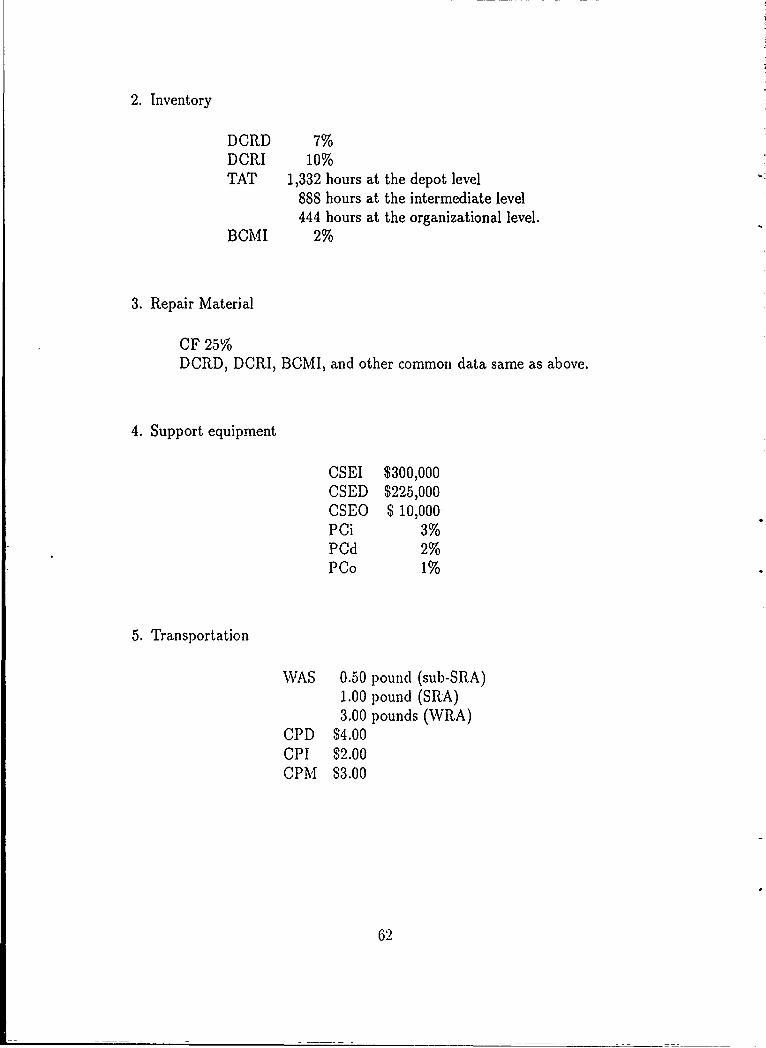
2. Inventory
DCRD 7%DCRI 10%TAT 1,332 hours at the depot level
888 hours at the intermediate level444 hours at the organizational level.
BCMI 2%
3. Repair Material
CF 25%DCRD, DCtII, BCMI, and other common data same as above.
4. Support equipment
CSEI $300,000CSED $225,000CSEO $10,000PCi 3%PCd 2%PCo 1%
5. Transportation
WAS 0.50 pound (sub-SRA)1.00 pound (SRA)3.00 pounds (WRA)
CPD $4.00CPI $2.00CPM 83.00
62

6. Training
DHPD 70% x 8 hours =5.6 hoursEDPY 300 daysCPT $5,000ATR 3%
7. Discount factor
y = 15 years at? = 10%:
DI 1 I+0.1-1 = 7.6
8. Annual Failure
ANF = NxFx365 Nx24x365 _8760N
MTBF IT.BF MIT BF
The values of N and MITBF are:
Nr = 160 for each assembly.AITBF = 5000 hours = MTTBF1 (WRA 1.2);
= 15000 hours = MTTBF 2 (SRA 1.2.1);= 7500 hours = MITBF3 (SRA 1.2.2);= 12000 hours = AITBF4 (Sub-SRA 1.2.2.1);= 20000 hours = MITBF5 (Sub-SRA 1.2.2.2).
The relationship between these MITBF values are [Ref. 10:Ch. 2 and 5]:
1/MITBF1 = 1/MITBF,2 + 1/A'ITBF,3
01,
1/5,000 =1/15, 000 + 1/7,500;
G3

1/MTBF3 = 1/MTBF4 + 1/MTBF
or
1/7,500 = 1/12,000 + 1/20, 000.
9. The unit costs are:
Unit cost (UC) of a WRA = $600.00Unit cost (UC) of an SRA = $300.00Unit cost (UC) of a sub-SRA = $150.00
B. LIFE-SUPPORT COST COMPUTATION
Based on the equations developed in Chapter IV, the life-support costs
are computed for each category. The first step is to compute the values of
Ncd, Nci, and Nco that will be used in the cost equation.
The next step is to compute the total cost of each assembly for each
maintenance alternative. With these results, the total costs for each alterna-
tive in Appendix A can be computed.
Using the fermula in Chapter IV, the values of Ncd, Nci, and Nco can
be computed for the specified values of N and MTBF. For N=160 and
MTBF=20,000 hours and depot level repair (TAT=1,332 hours),
K N x TAT/MTBF = 160 x 1,332/20,000 = 10.656 failures
Therefore, the probability of x sub-SRAs failing is:
p(qr) = (106.56)r6-10656
X!
64
---- -- --- -----

We will assume that the protection level required is 0.95; therefore, we
want the smallest value of Ncd such that P(x < Ncd) > 0.95. From Table 5.1
we see that the value of Ncd is 16.
Similarly, for the specified values of N and MTBF, the values of Ncd,
Nei, and Nco are computed and the results are listed in Tables 5.2.
6.5

TABLE 5.1: Poisson Probability Distribution for Computing Ned
p(x) jf=p(x) = P(x Ncd)0 0.000024 0.0000241 0.000251 0.0002752 0.001338 0.0016123 0.004751 0.0063634 0.012657 0.0190205 0.026974 0.0459946 0.047906 0.0939007 0.072927 0.1668278 0.097138 0.2639659 0.115012 0.378977
10 0.122557 0.50153411 0.118724 0.62025812 0.105427 0.725685
13 0.086418 0.81210314 0.065776 0.87787915 0.046727 0.924606
=16 0.031120 0.955727
TABLE 5.2: Values of Ned, Nci, and Nco
N =160TAT (hours) MTBF (hours) 5,000 7,500 12,000 15,000 20,000
13,320 Ncd = 45 37 25 21 16888 Nci = 37 26 18 15 12444 Nco = 19 15 10 9 7
66

Based on the cost equations developed in Chapter IV, the present value
of the various total costs for each alternative can be written for general UC,
Ncd, Nci, Nco, WAS, and MTBF.
1. Discard Alternative
NMPCO = 8760x x0.5x5x7.6
MTBFN
= $1 66 ,4 4 0 MTBF
NINVCO = (Nco + 8760 X MTBF X 7.6) x UC
N= (Nco + 66 ,576 MTBF) x UC
SECO = 10,000 x (1+ 0.01x 7.6)
= $10,760
TRNICO = 8760 x -- x 0.5/(5.6 x 300)] (1 + 0.03 x 7.6) x 5,000N
= $1 6 , 00 4 .52 MTBF
Total costs for the discard alternative:
N
TCO = $10,760+182,444.52x NMTBF
N+(Nco + 66,576 x MTB) x UC
2. Depot Alternative
NMPCD = 8760 x MTBF(3 x60+0.8x20+0.5x50) x7.6
N= $13 ,215, 3 36MTBF
67

NINVCD = (Ncd + 8760 x MTBF x 0.07 x 7.6) x UC
N= (Ncd+ 4 ,6 6 0.3 2 MTBF) x UC
RMCD = [Ncd + 8760 MN_(1- 0.07) x 7.61 x 0.25 x UC
= (0.25Ncd+ 15,478.92 NMTBF) X U
SECD = 10,760 + 225,000 x (1 + 0.02 x 7.6)
= $269,960
NTRPCD = 8760 x -TBF x WAS x 7.6 x 4.00
N= $266,304 x WAS x
XMiTBF
Total costs for the depot alternative:
N NTCD = $269,960 + 13,215,336 x + 266,304 x WAS x
MTBF MTBFN
+(1.25 x Ncd + 20,139.24 MTBF) x UC
3. Intermediate Alternative
N
= $6,930,561.6MTB
IAVCI = Nci + 8760 x BF(0 .1 +0.02) x 7.6 x UCI ~MTBF
= (Nci.+ 7, 98 9 .12 MTB) x UC
RICI = [Aci + 8760 x N 11 - (0.1 + 0.02)) x 7.6] x 0.25 x UCN
= (0.25Nci + 14,6 t 6.7 2 MTBF ) x UC
68

SECI = 10, 760 + 300,000 x (1 + 0.03 x 7.6)
= $379,160
TRPCI = 8760 x NF(2.00 + 0.02 x 3.00) x WAS x 7.6MTBF 2 0 +
N= $137,146.56 x WAS x MTBF
TRNCI = 8760 x MTBF x 5/(5.6 x 300)] (1 + 0.03 x 7.6) x 5,000N
= $160,080.24 N MTBF
Total costs for the intermediate alternative:
NTCI = $379,160 + 7,090,641.84 x jqTBF + 137, 146.56 x WAS
N Nx MTBF + (1.25Nci + 22,635.84 x MTBF ) x UC
For the MTBF and UC values shown on page 70 and an N = 160
the present value of the total costs of each assembly for each maintenance level
can be computed (The Ncd, Nci, and Nco values are obtained from Table 5.2).
4. Total Cost for Assembly 1.2 (WRA)
TCD = 269,960 + 13,215,336 x 160/5000 + 266, 304 x 3.00 x 160/5000+(1.25 x 45 + 20,139.24 x 160/5000) x 600
= 81,138,839.74TCI = 379,160 + 7,090,641.84 x 160/5000 + 137,146.56 x 3.00 x 160/5000
+(1.25 x 37 + 22,635.84 x 160/5000) x 600= $1,081,584.74
TCO = 10,760 + 182,444.52 x 160/5000 + (19 + 66,576 x 160/5000) x 600= $1,306,257.42
69

5. Total Cost for Assembly 1.2.1 (SRA)
TCD = 269,960 + 13,215,336 x 160/15000 + 226,304 x 1.00 x 160/15000
+(1.25 x 21 + 20,139.24 x 160/15000) x 300= $486,084.73
TCI = 379,160 + 7,090,641.84 x 160/15000 + 137,146.56 x 1.00 x 160/15000+(1.25 x 15 + 22,635.84 x 160/15000) x 300
= $534,316.10
TCO = 10,760 + 182,444.52 x 160/15000 + (9 + 66,570 x 160/15000) x 300= $228,449.27
6. Total Cost for Assembly 1.2.2
TCD = 269,960 + 13,215,336 x 160/7500 + 226, 304 x 1.00 x 160/7500
+(1.25 x 37 + 20,139 x 160/7500) x 300= $700,334.46
TCI = 379,160+ 7,090,641.84 x 160/7500+ 137,146.56 x 1.00 x 160/7500
+(1.25 x 26 + 22,635.84 x 160/7500) x 300= $687,972.20
TCO = 10,760+ 182,444.52x 160/7500+(15+66,576x 160/7500) x 300= $445,238.55
7. Total Cost for Assembly 1.2.2.1
TCD = 269,960 + 13,215,336 x 160/12,000 + 226,304 x 0.50 x 160/12,000
+(1.25 x 25 + 20,139.24 x 160/12,000) x 150= $492,905.82
TCI = 379,160+7,090,641.84 x 160/12,000+ 137,146.56 x 0.50 x 160/12,000
+(1.25 x 18 + 22,635.84 x 160/12000) x 150= $523,262.88
TCO = 10,760+ 182,444.52 x 160/12,000+(10+66,576 x 160/12,000) x 150
= $147,844.59
8. Total Cost for Assembly 1.2.2.2
TCD = 269,960 + 13,215.336 x 160/20,000 + 226,304 x 0.50 x 160/20,000
+(1.25 x 16 + 20, 139.24 x 160/20,000) x 150= S403,914.99
70

TCI = 379,160 + 7,090,641.84 x 160/20,000 + 137, 146.56 x 0.50 x 160/20,000
+(1.25 x 12 + 22,635.84 x 160/20,000) x 150
= $465,846.73
TCO = 10,760 + 182,444.52 x 160/20,000 + (7+ 66,576 x 160/20,000) x 150
= $93,160.76
Based on the Appendix A alternatives, the present value of the
total life cycle costs associated with each LOR code assignment are computed
and are presented in Appendix B. In Appendix B the lowest total life-cycle
maintenance cost is $1,996,279 for alternative number 37. Therefore, the LOIh
assignments for the Driver assemblies should be:
e Assembly 1.2: intermediate maintenance level (I)
* Assembly 1.2.1: discard (X)
* Assembly 1.2.2: discard (X)
* Assembly 1.2.2.1: discard (X)
* Assembly 1.2.2.2: discard (X)
How close are other alternatives? For example, consider a complete
discard alternative (number 5) with total costs of $2,220,951. This cost is
11% higher than the optimal alternative (number 37). Thus, if the complete
discard alternative were chosen, it would be definitely more costly. Consider
the next alternative number 23, repair at the depot level of the WRA, and
discard of the SRAs and sub-SRAs. The total costs of this alternative are
$2,053,533, only 2.8% higher than the optimal alternative. This alternative
might be worth choosing instead of the optimal alternative, especially if the
number of maintenance personnel at the intermediate level is not adequate. In
71

addition, the maintenance personnel at the intermediate level could perhaps
be shifted to other activities since repair of the WRA is performed by the
contractor. Thus, a cost saving could result which was not actually part of
the LOR model. This near optimal solution presented to a decision maker
allows him to incorporate his knowledge about other aspects of the problem
in making a final decision.
72

VI. SUMMARY, CONCLUSIONS, andRECOMMENDATIONS
A. SUMMARY
This thesis develops the level of repair (LOR) analysis model for the case where
weapon systems have already been designed by some other country and are being
used by the Indonesian Navy. This model incorporates the existing maintenance
levels of the Indonesian Navy and allows for weapon system indenture levels. Using
this model, the present value of the total life-cycle costs for each indenture level
and its maintenance level alternative can be computed. From summing these total
life-cycle costs for each alternative, the optimal LORB assignment can be determined
for each indenture level.
B. CONCLUSIONS
1. The most important factors in the procurement decision process are life-cycle
costs (LCC), system effectiveness and the equipment being considered. The
life-support costs (LSC) are a significant part of LCC, especially for the navies
of developing countries which usually buy weapon systems that have already
been designed and produced by the industrial country. The model developed in
this thesis allows LOR analysis for any developed system that the Indonesian
Navy wishes to buy.
2. The framework of the LOR analysis presented in this thesis can be applied in
thc Indoncsian Navy because it was purposely dcsigned-to consider the current
maintenance levels of the Indonesian Navy.
73

3. The Indonesian Navy plans to become involved in system design development
at its national shipyard as a consequence a program of frigate building based on
licensing agreements from various industrial countries. Involvement in system
design during the weapon systems acquisition process would be a major step
toward increasing the Indonesian Navy's logistics planning capability, but a
more elaborate LQR model will be needed when this occurs.
4. There are some potential constraints in the short run. Obtaining access to re-
liability and maintainability data for the weapon system being purchased may
be difficult. Maintainability and material support data may also difficult to
access. The model may be incomplete when application is attempted. Com-
puter programming of the model will be necessary and may take considerable
time.
C. RECOMMENDATIONS
The LOR model proposed in this thesis should be used by the Indonesian Navy
as a first step in evaluating the life-cycle support costs for weapon systems purchased
from- other countries and should be the best method for maintaining such systems.
In addition to those constraints mentioned in Conclusion 4 above, several other
important aspects must be considered before the model can be used. These include:
the level of protection desired for spares and repair parts, how to determine the new
system's maintenance parameters (MTBF, required maintenance hours, indenture
levels, etc.) after the Indonesian Navy buys the system, transportation times and
costs between organizational, intermediate, and depot levels, expected discard rates
at the intermediate and depot levels, and repair material and support equipment
cost factors. Because of the size of the effort to implement this model, a project
team needs to be formed. Such a team should include cost analysts, operations
74

analysts, and computer scientists, as well as experts from the current supply and
maintenance organizations.
75

APPENDIX AThe Possible Alternatives of LOR Assignment
AssembliesWRA SRA Sub-SRA
Alternative 1.2 1.2.1 1.2.2 1.2.2.1 1.2.2.2(1) (2) (3) (4) (5) (6)
1 D T) D D D2 D D D X D3 D D D D X4 D D X - -
5 X ....6 I D I I I7 1 D I D DS I D i I D9 I D I D I10 I D I I X11 I D I X I12 I D I D X13 I D I X D14 I D I X X15 I D D D D16 I D D D X17 I D D X Dis I D D X X19 I D X - -
20 D X D D D21 D X D X D22 D X D D X23 D X X - -
24 I X I I I25 1 X I D D26 I X I I D27 1 X I D I28 1 X I I X29 I X I X I
76
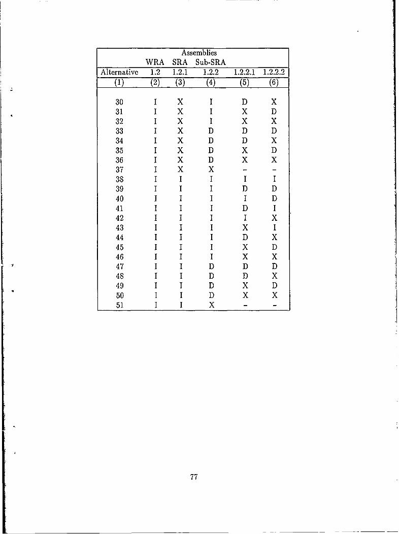
AssembliesWRA SRA Sub-SRA
Alternative 1.2 1.2.1 1.2.2 1.2.2.1 1.2.2.2(1) (2) (3) (4) (5) (6)
30 1 X I D X31 1 X I X D32 1 X I X X33 1 X D D D34 1 X D D X35 1 X D X D36 1 X D X X37 1 X X- -
38 1 1 1 1 139 I I I D D40 1 D41 1 D I42 I III X43 1 I 144 1 D X45 1 I I X D46 1 I I X X47 1 D D D48 1 D D X49 1 1 D X D50 1 D X X51 1 IX--
77
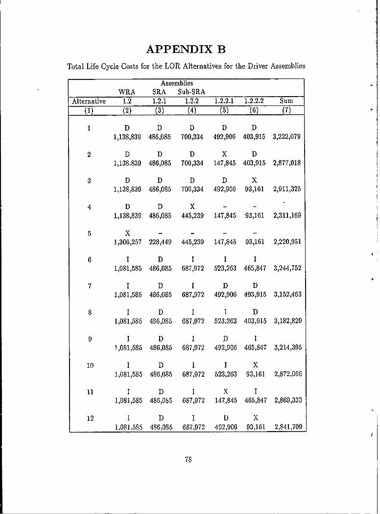
APPENDIX B
Total Life Cycle Costs for the LOR Alternatives for the Driver Assemblies
AssembliesWRA SRA Sub-SRA
Alternative 1.2 1.2.1 1.2.2 1.2.2.1 1.2.2.2 Sum(1) (2) (3) (4) (5) (6) (7)
1 D D D D D1,138,839 486,085 700,334 492,906 403,915 3,222,079
2 D D D X D1,138.839 486,085 700,334 147,845 403,915 2,877,018
3 D D D D X1,138,839 486,085 700,334 492,906 93,161 2,911,325
4 D D X -
1,138,839 486,085 445,239 147,845 93,161 2,311,169
5 x ..
1,306,257 228,449 445,239 147,845 93,161 2,220,951
6 I D I I I1,081,585 486,085 687,972 523,263 465,847 3,244,752
7 I D I D D1,081,585 486,085 687,972 492,906 403,915 3,152,463
8 I D I I D1,081,585 486,085 687,972 523,263 403,915 3,182,820
9 1 D I D I1,081,585 486,085 687,972 492,906 465,847 3,214,395
10 I D I I X1,081,585 486,085 687,972 523,263 93,161 2,872,066
11 I D I X I1,081,585 486,0b5 687,972 147,845 465,847 2,869,333
12 I D I D X1,081,585 486,085 687,972 492,906 93,161 2,841,709
78
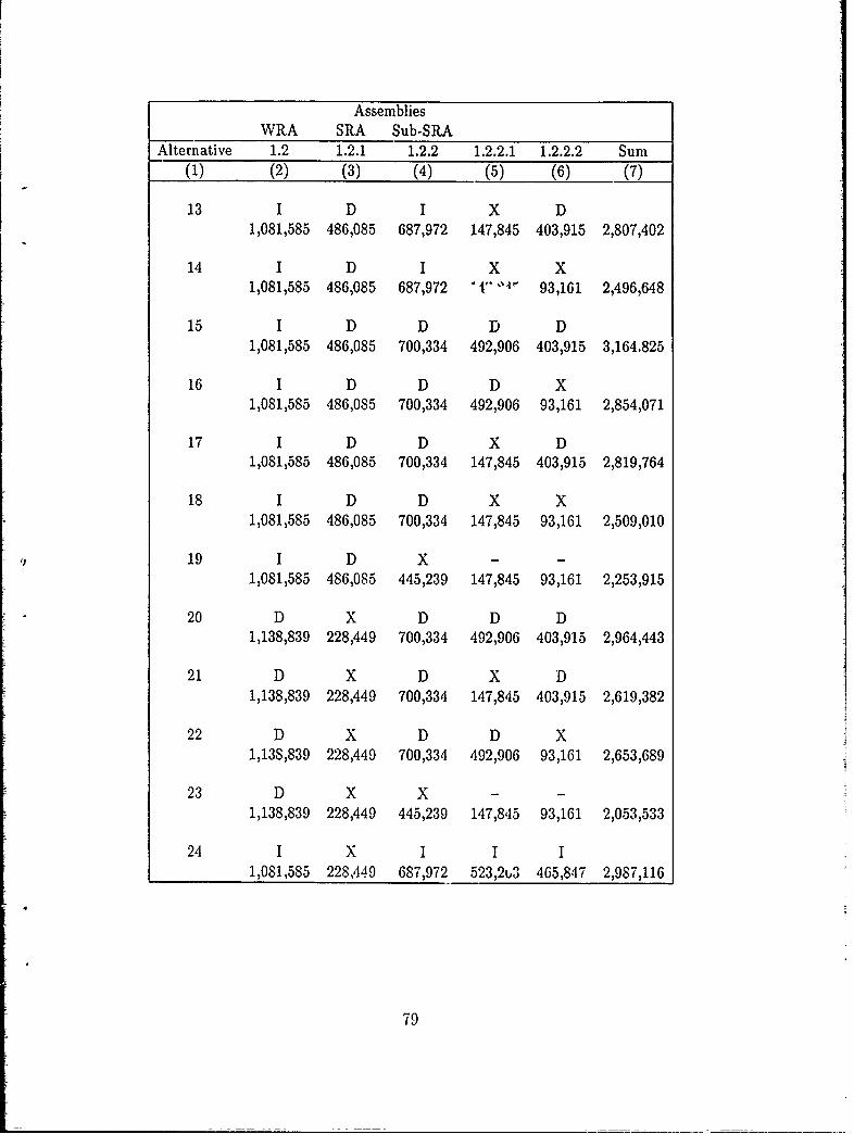
AssembliesWRA SRA Sub-SRA
Alternative 1.2 1.2.1 1.2.2 1.2.2.1 1.2.2.2 Sum(1) (2) (3) (4) (5) (6) (7)
13 I D I X D1,081,585 486,085 687,972 147,845 403,915 2,807,402
14 I D I X X1,081,585 486,085 687,972 i -r 93,161 2,496,648
15 I D D D D1,081,585 486,085 700,334 492,906 403,915 3,164.825
16 I D D D X1,081,585 486,085 700,334 492,906 93,161 2,854,071
17 I D D X D1,081,585 486,085 700,334 147,845 403,915 2,819,764
18 I D D X X1,081,585 486,085 700,334 147,845 93,161 2,509,010
19 I D X - -1,081,585 486,085 445,239 147,845 93,161 2,253,915
20 D X D D D1,138,839 228,449 700,334 492,906 403,915 2,964,443
21 D X D X D1,138,839 228,449 700,334 147,845 403,915 2,619,382
22 D X D D X1,138,839 228,449 700,334 492,906 93,161 2,653,689
23 D X X - -1,138,839 228,449 445,239 147,845 93,161 2,053,533
24 I X I I I1,081,585 228,449 687,972 523,2t,3 465,847 2,987,116
79

AssembliesWRA SRA Sub-SRA
Alternative 1.2 1.2.1 1.2.2 1.2.2.1 1.2.2.2 Sum(1) (2) (3) (4) (5) (6) (7)
25 I X I D D1,081,585 228,449 687,972 492,906 403,915 2,894,827
26 I X I I D1,081,585 228,449 687,972 523,263 403)115 2,925,184
27 I X I D I1,081,585 228,449 687,972 492,906 465,847 2,956,759
28 I X I I X1,081,585 228,449 687,972 523,263 93,161 2,614,430
29 I X I X I1,081,585 228,449 687,972 147,845 465,847 2,611,698
30 I X I D X1,081,585 228,449 687,972 492,906 93,161 2,584,073
31 1 X I X D1,081,585 228,449 687,972 147,845 403,915 2,549,766
32 I X I X X1,081,585 228,449 687,972 147,845 93,161 2,239,012
33 I X D D D1,081,585 228,449 700,334 492,906 403,915 2,907,189
34 I X D D X1,081,585 228,449 700,334 492,906 93,161 2,596,435
35 I X D X D1,081,585 228,449 700,334 147,845 403,915 2,562,128
36 I X D X X1,081,585 228,449 700,334 147,845 93,161 2,251.374
so

AssembliesWRA SRA Sub-SRA
Alternative 1.2 1.2.1 1.2.2 1.2.2.1 1.2.2.2 Sum(1) (2) (3) (4) (5) (6) (7)
37 I X X -
1,081,585 228,449 445,239 147,845 93,161 1,996,279
38 I I I I I1,081,585 534,316 687,972 523,263 465,847 3,292,983
39 I I I D D1,081,585 534,316 687,972 492,906 403,915 3,200,694
40 I I I I D1,081,585 534,316 687,972 523,263 403,915 3,231,051
41 I I I D I1,081,585 534,316 687,972 492,906 465,847 3,262,626
42 I I I I X1,081,585 534,316 687,972 523,262 93,161 2,921,296
43 I I I X I1,081,585 534,316 687,972 147,845 465,847 2,917,565
44 I I I D X1,081,585 534,316 687,972 492,906 93,161 2,889,940
45 I I I X D1,081,585 534,316 687,972 147,845 403,915 2,855,633
46 1 I I X X1,081,585 534,316 687,972 147,845 93,161 2,544,879
47 I I D D D1.081,585 534,316 700,334 492,906 403,915 3,213,056
48 I 1 D D X1,081,585 534,341 700,334 492,906 93,161 2,902,327
81

AssembliesWRA SRA Sub-SRA
Alternative 1.2 1.2.1 1.2.2 1.2.2.1 1.2.2.2 Sum(1) (2) (3) (4) (5) (6) (7)
49 I I D X D1,081,585 534,316 700,334 147,845 403,915 2,867,995
50 I I D X X1,081,585 534,316 700,334 147,845 93,161 2,557,241
51 I I X -
.1,081,585 534,316 445,239 147,845 93,161 2,302,146
82

APPENDIX C
A Glossary of Abbreviations and Acronyms
AASS = Average annual system stock quantity
ADT = Administrative delay time
ADHR = Annual duty hours per person
ANF = Average annual failures of an item
ATR, = Personnel attrition rate
BCM = Beyond capability of maintenance rate
BCMI = BCM rate at the intermediate level
BUFR = Buffer assembly
CF = Cost factor as a percentage of th, unit cost of module
CP = Shipping cost per pound
CPT = Training cost per person
CSE = Initial cost of support equipment
D = Depot level
DF = Discount factor
DCR = Discard rate
DHPD = Duty hours per person per day
DRIV = Driver assembly
EDPY = Effective repair days per year
F = Average operating hours per module per day
83

FDBLR = First doubler assembly
HR = Hourly labor rate
= Intermediate level
ILS = Integrated logistic support
INVC = Total life-cycle inventory costs
JRMC = Initial repair material costs
ITRNC = Initial training costs
LCC = Life-cycle cost
LDT = Logistic delay time
LSA = Logistic support analysis
LSC = Life-support cost
LOR = Level of repair analysis
M = Mean active maintenance time
M)T = Maintenance downtime
MHR = Manhours per action
MIL-STD = Military standard
MOD = Modulator assembly
MPLR = Multiplier assembly
MTBF = Mean time between failures
N = Number of application of identical modules in a systemmultiplied by the number of systems per operational site,and multiplied by the number of operational sites.
84

Nc = Number of spare modules as a protection level during
turn around time or inventory resupply time
0 = Organizational level
OSC = Oscillator assembly
PA = Power amplifier assembly
PSA = Power supply assembly
PC = Percentage of the initial support equipment costs
RIV..C = Total life-cycle repair material costs
SDBLI = Second doubler assembly
SEC = Total life-cycle support equipment costs
SRA = Shop replaceable assembly
TAT = Turn around ':me or inventory system resupply time
TRNC = Total life-cycle training costs
TRPC = Total life-cycle transportation costs
TSI = Time spent at intermediate level for each failure
TSO = Time spent at organizational level for each failure
UC = Unit cost of module
WAS = Weight of an assembly in pounds
WRA = Weapon replaceable assembly
X = Discard at failure
8.5

LIST OF REFERENCES
1. Jane's Fighting Ships, 1950-1951.
2. Sukardono, G., A Comparison of the Ship Acquisition Process of the In-donesian Navy and United States Navy, Master's Thesis, Naval PostgraduateSchool, December 1978.
3. Budiono, H., A Framework of the Indonesian Navy's Implementation of thePlanned Maintenance System, Master's Thesis, Naval Postgraduate School,December 1985.
4. Jane's Fighting Ships, 1987-1988.
5. Indonesian Navy, Pola Pembinaan Bidang Materil, PUM-1.03, December1986.
6. Indonesian Navy, Pola Dasar Pembinaan TNI-AL, PUM-1, December 1986.
7. Indonesian Navy, Pokok-Pokok Organisai dan Prosedur TNI-AL, March 1984.
8. Nielson, V.D., and Shahal, H., Application of Life Support Costs, Master'sThesis, Naval Postgraduate School, December 1981.
9. Kline, M.B., Maintainability Considerations in System Design, Doctoral dis-sertation, University of California, Los Angeles, 1966.
10. Blanchard, Benjamin S., Logistics Engineering and Management, 3rd edition,Prentice Hall, Inc., 1986.
11. Goldman, A.S., and Slatte.. T.B., Maintainability: A Major Element ofSystem Effectiveness, 2nd edition, John Wiley & Sons, Inc., 1967.
12. U.S. Department of Defense, Military Standard MIL-STD-1390, Level of Re-pair, 1987.
86

INITIAL DISTRIBUTION LIST
No. of Copies
1. Defense Technical Information Center 2Cameron StationAlexandria, Virginia 22304-6145
2. Library, Code 0142 2Naval Postgraduate SchoolMonterey, California 93943-5002
3. Defense Logistics Studies Information ExchangeU.S. Army Logistics Management CenterFt. Lee, Virginia 23801
4. Professor Alan W. McMastersCode 54MgDepartment of Administrative SciencesMonterey, California 93943-5000
5. Professor Kent AllisonCode 54AnDepartment of Administrative SciencesMonterey, California 93943-5000
6. CDR. Denny S. Partasasmita 2Komplek Hankam Sukabumi-Ilir No. 81JL. Kebayoran Lama-PalmerahJakarta, Indonesia
-. 8
87